The analysis of interaural time differences in the chick brain stem

Abstract

The brain stem auditory system of the chick has proven to be a useful model system for analyzing how the brain encodes temporal information. This paper reviews some of the work on a circuit in the brain stem that compares the timing of information coming from the two ears to determine the location of a sound source. The contralateral projection from the cochlear nucleus, nucleus magnocellularis (NM), to nucleus laminaris (NL) forms a delay line as it proceeds from medial to lateral across NL. NL neurons function like coincidence detectors in that they respond maximally when input from the two ears arrive simultaneously. This arrangement may allow NL to code sound space by the relative level of activity across the nucleus. The head anatomy of the chick allows for enhancement of the functional interaural time differences. Comparing the functional interaural time differences to the length of the neural delay line suggests that each NL can encode approximately one hemifield of sound space. Finally it is suggested that inhibitory input into the NM–NL circuit may provide a means to dynamically adjust the gain of the circuit to allow accurate coding of sound location despite changes in overall sound intensity.

Temporal information is important in the auditory system both for identification of different sources of sound and for determining the location of sounds. Identification of different sound sources can be accomplished, to a large extent, using monaural cues. While localization of a sound source can also be accomplished, to some extent, with only one ear, significant localization cues are contained in the comparison of binaural information. Sounds located to one side will arrive at the near ear slightly before they arrive at the distant ear and, in general, these offset sounds will be slightly louder in the near ear than in the distant ear. By analyzing differences in the timing and intensity of information at the two ears, the brain can compute the location of a sound source.

The circuitry for computing the location of a sound source begins in the brain stem. This report will review some of our work over the past several years on the circuit that begins the neural analysis of interaural time differences in the chick. Emphasis will be given to the anatomical, physiological and neurochemical adaptations in this model system to accomplish binaural sound localization. This manuscript is not meant to be an exhaustive review of the literature in the field, but rather, a story that exemplifies how adaptations at different levels of a system each contribute to enhancing the precision of an important task.

1. The circuit: anatomy

Jeffress [1] proposed what has become the classic model for encoding information relating to interaural time differences. This model, shown in Fig. 1A, provides a circuit for transforming time differences at the two ears into a place of maximal activation along an array of neurons. There are two main features of this model: 1) delay lines to an array of neurons and 2) neurons that function as coincidence detectors. As will be described later, both of these features hold true for a circuit in the brain stem auditory system of the chick.

Fig. 1.

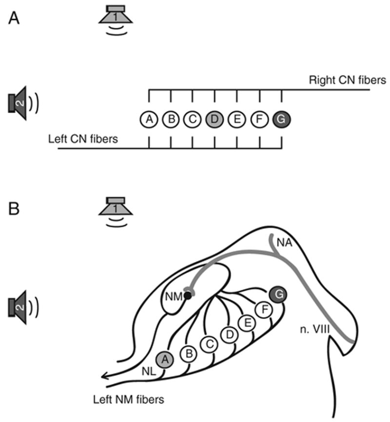
Models of how the brain might process interaural time differences. A. A version of the classic Jeffress model [1] with two opposing delay lines converging on an array of postsynaptic coincidence detectors. When the sound source is at midline (Speaker 1), information from the left and right cochlear nucleus (CN) fibers will reach Cell D simultaneously, whereas when the sound source is off to the left side (Speaker 2), action potentials begin in the left CN first and information from the two sides will arrive at Cell G simultaneously. Consequently, sound location is translated to a neural location of coincidence along the array of neurons. B. The circuit for coding interaural time differences in the chick brain stem. Auditory nerve fibers (n. VIII) enter the brain stem and bifurcate, sending one branch to nucleus angularis (NA) and another branch to nucleus magnocellularis (NM). NM fibers project bilaterally to nucleus laminaris (NL). In contrast to the Jeffress model, it appears that delay lines exist only in the contralateral projection to NL. The ipsilateral projection from NM to NL appears to splay out along the line of NL neurons such that axonal lengths to all areas are approximately equal. The contralateral projection, however, has a systematic increase in axonal length as the fiber proceeds from medial to lateral across NL. Estimates of the transmission delays suggest that when sounds are located near midline (Speaker 1), medial cells (Cell A) will receive input from the two NM at the same time, whereas when the sound is off to the contralateral side (Speaker 2), laterally placed NL neurons will receive coincident input (Cell G).

If a sound is located directly in front of an animal, then information about that sound will arrive at the two ears simultaneously. Assuming that the timing of the acoustic stimulation is preserved in the cochlear transduction process and in the early stages of neuronal processing, then the information from both ears will travel down their axons toward the array of cells at the same time. The arrival of information at each cell along the array is systematically delayed because of the sequential arrangement of cells relative to these axonal projections (i.e., the axonal projections form ‘‘delay lines’’). In Fig. 1A, the length of the projection to each cell represents the transmission delay to each cell. As a result of these opposing delay lines, information will arrive simultaneously at only one point along the array of postsynaptic neurons (cell D in the top schematic). If, however, a sound is displaced to one side of the head, then the sound wave will reach the near ear slightly before it reaches the distant ear. This would allow action potentials driven by the near ear to get a ‘‘head start’’ as they progress towards the array of cells. Consequently, information will arrive simultaneously at a different location along the array of neurons (cell G in this example). In this way, the delay lines transform the spatial location of a sound source to different places of simultaneous input on the array of neurons.

The pattern of innervation observed in the brain stem auditory system of the chick is similar to the circuit that Jeffress proposed. A systematic arrangement of axonal projections to an array of neurons was first described anatomically in the chick brain stem by Young and Rubel [2]. When the auditory nerve enters the chick brain stem, it bifurcates, sending one branch to nucleus magnocellularis (NM) and another branch to nucleus angularis (NA). Each neuron in NM then projects bilaterally to nucleus laminaris (NL). Neurons in NL are arranged, for the most part, as a curved monolayer of cells. These neurons have symmetrical dendritic processes oriented into distinct dorsal and ventral fields. Axons from the ipsilateral NM project to the dorsal dendrites and axons from the contralateral NM project to the ventral dendrites. Key to the present discussion is the orientation and pattern of these NM to NL projections. Both the ipsilateral and contralateral axons innervate an isofrequency line of neurons across NL. When looking at the ipsilateral projection to the array of NL neurons, there does not appear to be any ‘‘delay line’’ across the population of cells. The terminal branches of this projection appear to splay out across the line of cells such that axonal lengths are essentially equal across the isofrequency array. The projection from the contralateral NM, however, does appear to show a ‘‘delay line’’. Terminal branches from these axons emerge sequentially as the fiber projects from medial to lateral across the array of neurons (See Fig. 1B).

2. The circuit: physiology

Axonal length will determine the time it takes information to travel from the cell body to the terminal, but conduction time will also be influenced by variation in axonal width and myelination, features that are relatively difficult to examine anatomically. Even detailed anatomical measures will not provide an indication of how long it would take for the information to travel from one end of the array of postsynaptic neurons to the other. To confirm the presence of delay lines and to estimate the magnitude of the delay, we examined the delay line circuit of the NM to NL projections using a brain slice preparation of the chick auditory system [3]. A 400 μm para-coronal slice of the chick brain stem preserves this circuit and this slice of tissue can be maintained in vitro for physiological studies using standard techniques. NM was electrically stimulated while recording the evoked activity in NL at different locations along the medial to lateral extent of NL. As predicted by the anatomical studies, there was no systematic variation in the latency of response along the length of NL when the ipsilateral NM was stimulated (Fig. 2A). Stimulation of the contralateral NM, however, resulted in a linear increase in latency of the response as the recording location was moved from medial to lateral along the array of NL neurons (Fig. 2B). These data match the anatomical predictions and provide evidence for a delay line-like organization in the contralateral projection to NL.

Fig. 2.

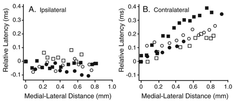
Delay Lines. Physiological measurements from a brain slice preparation of the chick auditory system confirm that delay lines exist only in the contralateral projection to NL. A. The recording electrode was placed at various medial to lateral locations in NL. There is little difference in the latency of action potentials reaching various NL locations when the ipsilateral NM is stimulated. B. In contrast, there is a near linear increase in the latency of responses across the medial to lateral extent of NL when the contralateral NM is stimulated. Different symbols represent the recordings made in different slices. These slices were maintained at 34 °C, giving a total delay across NL of approximately 300 μs. When recorded at physiological temperature (40–41 °C), a delay of approximately 180 μs is observed across the medial to lateral extent of NL (not shown). Data replotted from Ref. [3].

Although the Jeffress model proposed opposing delay lines in both directions to create a neural map for interaural time differences, it should be noted that this map can be readily created using a unilateral delay line with a constant delay in activation from the other side. This is diagramed in Fig. 1B. You will note that this schematic shows that sounds at midline are represented near the medial edge of the nucleus, rather than in the middle. This would mean that each NL would encode time delays generated by sounds emanating from the contralateral hemifield of possible locations, perhaps with bilateral representation of sounds located near midline. This estimate of the spatial receptive fields of each NL is based on the absolute measure of axonal delays as compared to absolute measurements of time delays between the two ears for sounds placed at different locations (see ‘‘Relationship to Physical Features of Sound’’, below). Measurements of absolute axonal conduction delays were performed in the brain slice preparation by recording the medial-most and lateral-most positions of the nucleus simultaneously while stimulating the contralateral projection to NL. These measurements revealed that the axonal delay across the medial to lateral extent of the nucleus would reach a maximum of approximately 180 μs when recorded at physiological temperatures. This matches the measurements of the physical interaural time difference produced by a sound located at 90° azimuth (see below).

Evolutionarily, the bias of coding towards the contralateral hemifield could have emerged because of limitations in conduction velocity. Action potentials from the contralateral NM have farther to travel than those from the ipsilateral NM, except for the most medially located NL neurons. Consequently, for sounds located at midline to be represented in the center of the array of neurons, the conduction velocity of the contralateral axons would have to be dramatically faster than that of the ipsilateral axons. This ‘‘limitation’’ of the coding range to a hemifield, however, allows for the possibility of greater precision of sound location across the limited array of neurons. This can be appreciated in the schematics in Fig. 1, where only 4 neurons code 90° azimuth in Fig. 1A, but 7 neurons code 90°in Fig. 1B.

3. Relationship to physical features of the sound

If this circuit encodes interaural time differences, then the coding range of the system should match the range of ITDs that is experienced by the bird. Interaural time differences, of course, will be largely determined by the size of the subject’s head. Given that chickens have small heads, one would expect that the range of ITDs available for coding sound location would be severely limited. Estimates of the length of the delay line formed in the contralateral projection to NL were approximately 180 μs [3]. This appears to be much larger than the maximal ITD possible (approximately 75 μs) based on calculations using the size of the chicken’s head and the speed of sound. Like many small-headed animals, however, chickens have an adaptation that serves to enhance the functional interaural time differences [4–6]. The middle ear cavities of the chick are acoustically coupled by an air-filled canal that joins the two cavities. In a sense, literally, what goes in one ear, comes out the other. The canal is formed by a connection of the two Eustachian tubes, which join together and open into the nasopharynx by a common orifice. Consequently, sound waves impinging on the tympanic membrane of one ear force that membrane forward, but force the contralateral tympanic membrane outward by the pressure transmitted through the interaural canal. This arrangement means that a sound in free field will have opposing forces on the tympanic membrane movement; the membrane will be forced inward from outside of the head and forced outward from pressure transmitted through the interaural canal. The sound traveling through the head and sound traveling around the head will have different pathlengths. This results in a phase interaction between the two pressure waves on the opposite sides of the membrane. The phase shift in the displacement pattern of the tympanic membrane is such that it accentuates the functional ITDs (and interaural intensity differences) for sounds presented in free field.

To test the hypothesis that the interaural canal serves to produce functional ITDs that are greater than those predicted simply by the size of the head, we measured functional ITDs by recording cochlear microphonic (CM) responses [7]. The CM is a cochlear potential that follows the waveform of a sound stimulus. The functional ITD was measured by performing a cross-correlation between the bilaterally recorded CMs. A sound source was moved to various azimuthal locations around the bird in an anechoic chamber and the CMs were recorded and analyzed. These data are displayed in Fig. 3. As expected, when the sound source was placed at midline, the cross-correlation revealed that the time difference was near zero. The maximal ITD recorded was, of course, when the sound was place 90° off to one side of the head. Interestingly, the maximal ITD varied depending on the frequency of the sound. For relatively low frequency sounds (<1 kHz) the maximal ITD was approximately 160–180 μs, which was much larger than the 75 μs ITD predicted simply by measuring the size of the head. For high frequency sounds, the augmentation of the functional ITD was relatively small, but reliable. This frequency-specific aspect of the data agreed with the results obtained for a variety of other birds [4] and it is thought to represent a frequency-dependent impedance of pressure waves transmitted through the interaural canal.

Fig. 3.

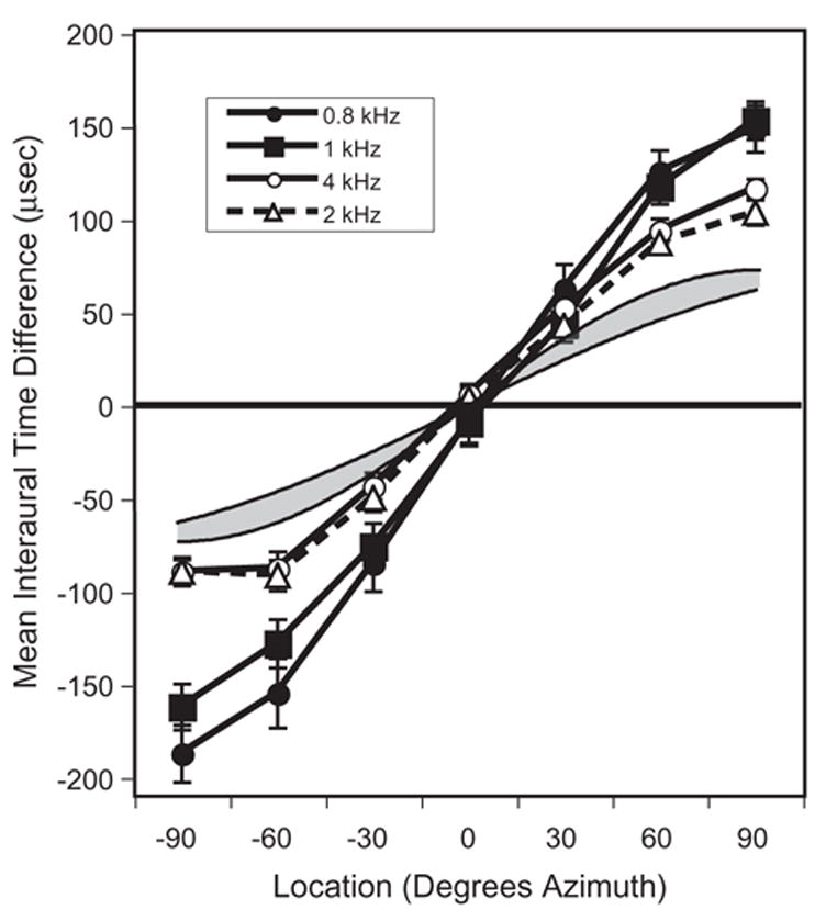
Augmentation of Functional ITDs. Interaural time differences between cochlear microphonic responses in the two ears of a chick as location of the sound source was moved in azimuth. The gray area between the curved lines represents the range of theoretically maximal ITDs that would be expected based on the distance between the two ears (models of Kuhn [32] and Woodworth [33]). The measured ITDs were much greater than the predicted ITDs, particularly for low frequency sounds. Data replotted from Ref. [7], bars represent standard error of the mean.

To determine if the augmentation of functional ITDs results from the acoustic coupling of the middle ear cavities, we measured the change in the CM before and after occluding one ear canal. CMs were measured from the ear distal to the sound source. When the canal for the contralateral ear (the ear closest to the sound source) was occluded, the CM from the open (distal) ear occurred sooner and increased in amplitude (Fig. 4A). These effects, just like the augmentation of functional ITD, were frequency dependent such that larger effects were seen with low frequency sounds (Fig. 4B). While this review is focused on ITD cues, it should be noted that this experiment demonstrates that the interaural canal enhances interaural intensity differences as well, bringing both cues to a range that could be better utilized by the bird to determine the location of a sound source.

Fig. 4.

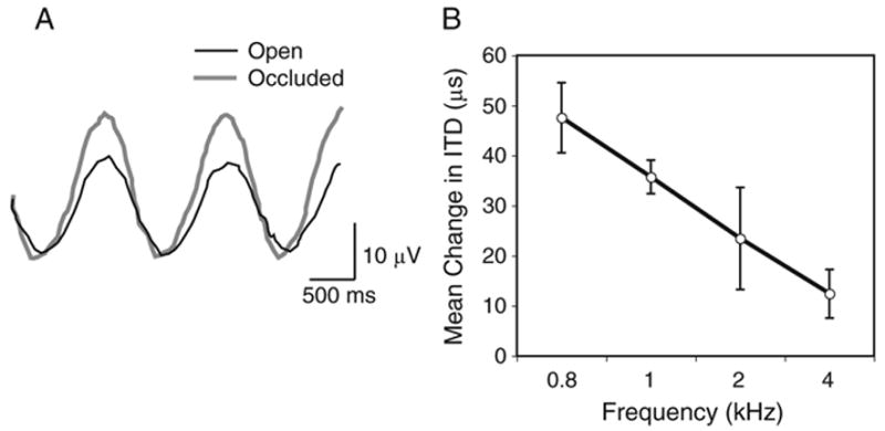
Augmentation of ITD is attributable to interaural canal. A. Example of the effects of occluding one ear on the cochlear microphonic (CM) response of the contralateral ear. A sound source was placed at 90° azimuth and CM responses were recorded in the distal ear. When the ear near the sound source was occluded, the CM in the distal ear became larger and occurred earlier. This indicates that sound transmission through the interaural canal enhances functional ITDs. B. The mean change in time of the CM when the contralateral ear was occluded was greatest for low frequency sounds. Data replotted from Ref. [7], bars represent standard error of the mean.

One of the remarkable findings of these experiments was that the functional ITD measured by the cochlear microphonic response was closely matched to the estimate in the length of the delay line observed in our in vitro physiological studies of the NM to NL projection [3]. Together, these experiments suggest that each NL can encode approximately one hemifield of sound location in azimuth. This is the arrangement depicted in Fig. 1B.

4. Coincidence detection

Delay lines measurements confirm that action potentials (hence synaptic activation) arrive at different portions of the nucleus at different times, but for a Jeffress-like model to hold, NL neurons must also work as coincidence detectors. That is, their activity must be dependent on whether or not they simultaneously received the phase locked information about the acoustic stimulus from each NM. The capacity of NL neurons to function as coincidence detectors was also confirmed in the brain slice preparation [8]. Trains of stimulation pulses were applied bilaterally to the two NM while recording from single neurons in NL. The timing of stimulating the ipsilateral and contralateral NM was then systematically varied to simulate a range of potential interaural time differences that might occur if activity was driven by a sound in space. As expected, NL neurons respond as coincidence detectors; they are more likely to generate an action potential when the inputs from the two NM arrive at the same time. Fig. 5 shows an example of the change in response probability as the simulated interaural time difference (s-ITD) is varied. While unilateral input is capable of producing action potentials in NL neurons, the peak response of the NL neuron is much greater than the sum of the two unilateral probabilities. Intracellular studies show that indeed the NL neurons summate subthreshold excitatory post-synaptic potentials (EPSPs), produced by each NM input, to produce action potentials [9–12].

Fig. 5.

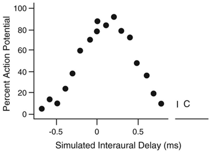
Coincidence detection. NL neurons can function as coincidence detectors. The responses of single NL neurons were measured in a brain slice while stimulating both the ipsilateral and contralateral inputs. Interaural time differences were simulated by varying the delay between the stimulation of the two inputs. As can be seen in this example, neurons showed a greater percentage of action potentials when inputs from the two NM arrive at the same time (s-ITD=0). I (ipsilateral) and C (contralateral) represent the percentage of action potentials evoked by unilateral stimulation. Data replotted from Ref. [8].

Although coincidence detection by NL neurons is well documented and fits with a Jeffress-like model, there are a few limitations to this simple conceptualization. One of the main limitations lies in the width of the s-ITD function. For an array of coincidence detectors to encode the location of a sound source by producing a peak area of activity, they must have ITD functions with extremely discrete peaks. In general, the recorded s-ITD functions have a relatively broad plateau at the peak of the curve. Typically the peak of the curve is much broader than the potential variation of delay across the nucleus produced by the delay lines. The slope of the ITD function, however, is relatively sharp so the transition from a maximal firing rate to a low firing rate does occur over a small variation in ITD. This observation led us to propose a slight modification to the simple Jeffress-like model [8]. Rather than the place code being based on the locus of a maximally firing unit, we proposed that the place code is based on the locus of the border between clusters of maximally firing units and minimally firing units across the array. A similar proposal for ITD coding in the mammalian auditory system has also been made based on the experimental and theoretical work of McAlpine and Harper and McAlpine et al. [13,14]. Fig. 6 illustrates our model based on the NL responses recorded in vitro. These responses were recorded at 34 °C, consequently, the ITDs will be much longer than would be the case in vivo (see Fig. 2) and it is likely that the shape of each cell’s function would be somewhat sharper in vivo. These temperature-dependent effects would produce quantitative differences in this model, but would not be expected to produce qualitatively different results. Fig. 6 shows a hypothetical array of three NL neurons. The s-ITD function of each is based on the function of a cell from our in vitro recordings. These cells are plotted to depict three cells in an array that receive simultaneous ipsilateral activation, but their contralateral activation is systematically delayed by 100 μs between each cell. This would be the case for cells located at different medial to lateral locations along a line of cells in NL, as represented in Fig. 1B. Consequently, the shape of each cell’s ITD function is identical but each function is offset by 100 μs. The width of the gray boxes highlights a change in s-ITD of 100 μs. The height of each box highlights the variation in response rate across the population of neurons. The box on the left is centered on the peak of the central cell’s s-ITD function, and the box on the right is centered on the point of this cell’s steepest slope. If ITDs were coded based on the peak of a cell’s response, there would be very little difference in the response rate across the population of neurons. All three neurons are near their maximum firing rate throughout the 100 μs variation in ITD. If, on the other hand, the slope of the ITD function coded sound location, then there is substantial variation in response rate across the population of neurons. In this model, no single cell provides unique information about the location of the sound source, but there is a border between maximally and minimally firing cells depending on the ITD. For example, when the s-ITD is 0.2 ms, two of the cells are firing near their maximum rate, but the third is near zero. Conversely, when the s-ITD is 0.3 ms, two of the cells are near zero, while the third is near its maximal firing rate.

Fig. 6.

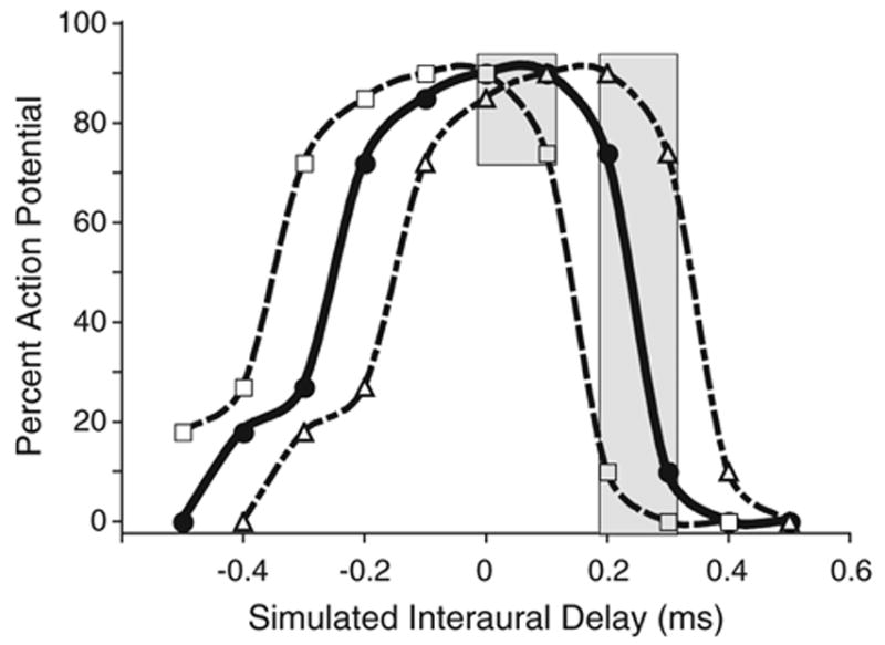
Population code model. Three hypothetical cells along nucleus laminaris with simulated interaural time difference curves based on the responses of cells recorded in a brain slice preparation. The peaks of the curves are placed 100 μs apart. The gray box on the left shows the inclusive variation in response rate that would be observed across a 100 μs change in delay. Very little variation in response rate across this population of cells would be observed if sound location was coded at the peak of these s-ITD curves. In contrast, the same 100 μs change in delay across the point of steepest slope (gray box on the right), would result is a large variation in response rate across the array of cells.

5. Neurotransmitter systems

Localizing sounds based on ITDs requires a system that can discriminate between different ITDs that vary by only a few microseconds. This is quite a challenge for a neural system since the electrical events of neurons are relatively slow. As a case in point, the maximum ITD in the chick is approximately 180 μs, but the duration of an EPSP in brain stem auditory neurons is approximately 500 μs. In the chick brain stem, specializations in ion channels and neuro-transmitter receptors allow for the enhanced accuracy of coincidence detection that is required to code for fine variations in ITD.

The model described above has focused solely on the excitatory pathways from the ear to NM and from NM to NL. This excitation is mediated by the neurotransmitter, glutamate. The glutamate receptors in NM and NL appear to be optimized for processing temporal information [15]. These receptors rapidly desensitize thereby limiting the duration of the EPSP. Briefer EPSPs would mean that very accurately timed information (coincidence) would be required in order for two EPSPs to summate to produce an action potential. Additionally, NM and NL neurons have a significant concentration of low threshold potassium channels [16]. These channels appear to assure accurate timing of action potentials and help speed the recovery to resting potential that is needed for rapid firing and phase locking [17]. These channels also appear to assure that only EPSPs that occur very near coincidence will summate to produce an action potential [18,19]. If one EPSP begins and the low threshold potassium current is activated, then the current from the second EPSP will be shunted and the cell will not reach threshold.

While the specializations of the physiological properties of the cells help optimize the circuit for the temporal processing of excitatory drive, NM and NL also receive a substantial GABAergic input in addition to the excitatory glutamatergic input [20,21]. The main source of the GABAergic input appears to be from fibers descending from the ipsilateral superior olive (SO) [22], but there is also a small population of GABAergic cells located between NM and NL that send processes into both nuclei [23]. The large GABAergic input to these areas begs questions about the possible role of this inhibitory input in temporal processing.

Activation of GABA_A receptors on both NM and NL neurons produces a depolarization [24,25]. This depolarization, however, is inhibitory in that it blocks action potentials evoked by stimulating the afferent axons and action potentials generated by injection of depolarizing current into the cell. It appears that both NM and NL neurons have a high internal Cl⁻ concentration resulting in a chloride equilibrium potential that is depolarized from resting potential. Evidence that the native Cl⁻ equilibrium potential is depolarized from rest comes from recordings using sharp electrodes filled with potassium acetate, that would not be expected to dramatically affect internal Cl⁻ concentrations [9] and from perforated patch clamp recordings [25]. The inhibition of action potentials most likely occurs because of the shunting of current produced opening the Cl⁻ channels and additional shunting owing to the opening of the low threshold K⁺ channels discussed above.

In both NM and NL, GABA could serve to enhance the neurons’ ability to preserve timed information [10,26,27]. The large decrease in input resistance increases the required amount of depolarizing current to bring the neurons to threshold. This means that only accurately timed EPSCs will summate to produce a current sufficient to generate an action potential.

The circuitry driving the activation of GABAergic input into NM and NL suggests that GABAergic ‘‘tone’’ may be related to the intensity of the acoustic stimulus. The superior olive neurons, which project to these nuclei, receive input from NL and the cochlear nucleus angularis (NA). As the intensity of an acoustic stimulus increases, the synaptic drive of SO neurons, particularly from NA, will also increase. Consequently, there will be greater release of GABA in NM and NL as sound intensity increases. One possible role of this recurrent inhibition is that it could serve to dynamically adjust the gain of the NM–NL timing circuit depending on the intensity of the acoustic stimulus. Indeed, in vivo data from the owl suggest that ITD sensitivity of NL neurons is relatively insensitive to changes in sound level [28].

It is easy to imagine how increased inhibition will counteract increased drive as sound level increases. This notion has been supported by in vitro studies which have shown that activation of SO produces a relatively long lasting inhibition of brain stem neurons [27]. We have found, however, that GABA could also lead to a counterintuitive increase in the gain of the system under certain circumstances. It appears that whether GABA increases or decreases the gain of the system depends on the amount of GABA present. Brückner and Hyson [9] generated single-unit s-ITD functions in vitro by stimulating the two inputs to NL while recording intracellularly with sharp electrodes. Application of a low concentration of GABA to the bath unexpectedly resulted in enhanced excitability of the NL neurons and a sharpening of the s-ITD function (Fig. 7A). Application of higher concentrations of GABA led to the traditional decrease in excitability of the NL neuron (Fig. 7B).

Fig. 7.

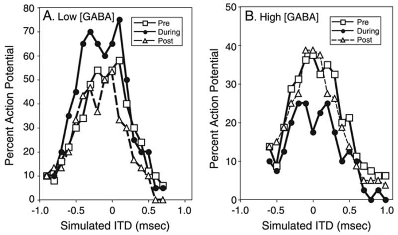
s-ITD functions and GABA. s-ITD functions recorded in a brain slice preparation before, during and after bath application of GABA. A. A low concentration of GABA (1.25 μM) increased the excitability of the NL neuron and sharpened the s-ITD function. B. A high concentration of GABA (10 μM) reduced the excitability of the NL neuron. Replotted from Ref. [9].

An increase in excitability was not observed by Yang et al. [27] when recording from NL neurons while stimulating the SO electrically. In these experiments, only a relatively long lasting inhibition was observed. There are several possible reasons for this apparent discrepancy. First, the experiments showing increased excitability were performed with K–acetate filled sharp electrodes while those that failed to observe the increased excitability were performed with whole cell patch clamp. Perhaps the alterations in Cl⁻ equilibrium potential produced by diffusion of the pipette solution into the cell in the whole cell configuration somehow prevented the observation of increased excitability. Second, the experiments showing increased excitability were preformed on young hatchling chicks while those failing to see increased excitability were performed on embryos. Perhaps there are changes in the receptors or other channels during this phase of development. Finally, the enhanced excitability was only observed with very low concentrations of GABA. Perhaps the synchronous stimulation of the SO results in too great of release of GABA to observe this phenomenon.

We have also observed increased excitability by low concentrations of GABA in NM of hatchling chicks [29,30]. Bidirectional effects have also been observed by Lu and Trussell [25]. Our first studies simply recorded evoked activity in NM using field potential recordings. The auditory nerve was electrically stimulated while GABA agonists and antagonists were applied. The field potential recordings showed that low GABA concentrations increase the excitability of NM neurons (larger postsynaptic fields), while higher concentrations have inhibitory effects. Intracellular recordings confirmed that GABA could both increase and decrease excitability. GABA depolarizes these neurons and action potentials were observed when a low dose of GABA was combined with subthreshold auditory nerve stimulation. Higher doses of GABA produced large depolarizations and blocked action potentials produced by suprathreshold auditory nerve stimulation. The increase in excitability produced by low doses of GABA (5 μM) appears to be mediated by GABA_A receptors. This response was blocked by the GABA_A antagonist bicuculline, and the increased excitability could not be induced by the GABA_B agonist baclofen. The inhibition produced by relatively high GABA concentrations (20 μM) appears to involve both GABA_A and GABA_B receptors. The GABA_B receptor antagonist 2-hydroxysaclofen partially blocked this inhibitory response and the residual inhibition was blocked by bicuculline.

The effects of GABA in NM are presented in Fig. 8. Fig. 8A displays the average change in field potential amplitude over time during bath application of different concentrations of GABA. Note that the size of the postsynaptic field potential driven by auditory nerve stimulation either increased or decreased depending on the concentration of GABA added to the bath. To observe the effects of GABA using intracellular recording, the auditory nerve was stimulated while recording from an NM neuron. In Fig. 8B, upward deflections indicate the action potentials recorded in current clamp. The downward deflections are produced by intracellular injection of current a short time after each stimulation pulse to the auditory nerve. These current injection pulses allow one to observe changes in input resistance produced by the GABA application. GABA was focally and transiently administered by brief pressure ejection of the drug from a nearby pipette into the bath. When the auditory nerve stimulation was subthreshold, a short pressure pulse of GABA resulted in a mild depolarization and the subthreshold inputs became suprathreshold (i.e., action potentials are now observed). When the auditory nerve stimulation was suprathreshold, a longer pressure pulse of GABA produced the widely observed depolarizing inhibitory effect.

Fig. 8.

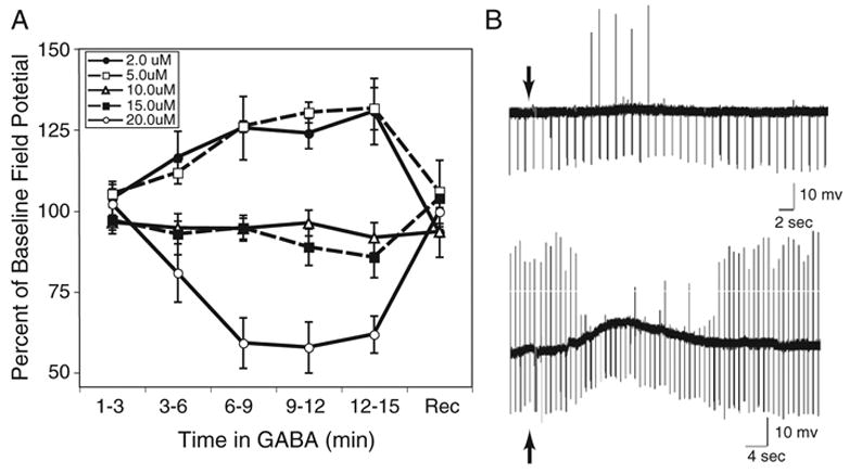
Bidirectional effects of GABA in NM. GABA either increases or decreases excitability of nucleus magnocellularis (NM) neurons. A. Changes in the amplitude of an averaged field potential recorded in NM following electrical stimulation of the auditory nerve at various times following the addition of GABA to the bathing medium. The field potentials are enhanced when a low concentration of GABA is added to the bath, but these potentials are reduced when a higher concentration of GABA is added to the bath. Rec. refers to the recovery of the field potential amplitude after return to the normal bathing solution. Bars represent standard error of the mean. B. Intracellular recordings from NM neurons during a brief application of GABA. Downward deflections are produced by intracellular current injections. Changes in the size of the negative voltage deflections reflect changes in input resistance of the cell. The auditory nerve was repeatedly stimulated, and the large upward deflections are action potentials produced by this afferent drive. When the auditory nerve stimulation was subthreshold, a small concentration of GABA resulted in a slight depolarization and the emergence of auditory nerve-driven action potentials (upper trace). When the auditory nerve stimulation was suprathreshold, application of a larger dose of GABA produced a pronounced depolarization and the inhibition of auditory nerve-driven action potentials (lower trace). GABA was applied by focal pressure injection into the media near the recorded cell at the time indicated by the arrows.

Together, the data from both NM and NL suggest that one role of GABA could be to dynamically regulate the gain of the ITD coding circuit. This does not preclude other roles of GABA, such as maintaining the temporal fidelity of firing under conditions of high rates of activity [10,31]. The inhibitory role of GABA under conditions of high amplitude stimulation is fairly intuitive and could be responsible for keeping the firing rate of neurons from saturation. This would allow coding of ITDs to be preserved regardless of sound intensity [28]. The boost in the gain of the system under low sound level conditions is speculative, but, if true, could serve to enhance localization ability for relatively soft sounds. This would be of obvious importance for animals if, for example, a predator was approaching.

6. Summary

A circuit in the brain stem of the chicken provides an exquisite example of how anatomy and physiology intertwine to accomplish an important task. First, the head anatomy allows for an enhancement of the interaural cues. Second, the neuroanatomy serves to systematically vary the physiological input to an array of neurons. Finally, these neurons have incorporated physiological features that optimize their performance for detecting coincident input. Together, the circuit enhances coding of binaural temporal information allowing, among other things, the localization of a sound source in space. The study of this system has advanced our knowledge of how the brain codes acoustic information, but it also serves as a valuable model for how the brain processes temporal information. Temporal processing is important throughout the brain, and this work raises the question of whether the features of the NM–NL circuit are ‘‘specialized’’ or if these features are common to multiple brain regions that code temporally sensitive information.

References

- 1.Jeffress LA. A place theory of sound localization. J Comp Physiol Psychol. 1948;41:35–9. doi: 10.1037/h0061495. [DOI] [PubMed] [Google Scholar]
- 2.Young SR, Rubel EW. Frequency-specific projections of individual neurons in chick brainstem auditory nuclei. J Neurosci. 1983;3:1373–8. doi: 10.1523/JNEUROSCI.03-07-01373.1983. [DOI] [PMC free article] [PubMed] [Google Scholar]
- 3.Overholt EM, Rubel EW, Hyson RL. A circuit for coding interaural time differences in the chick brainstem. J Neurosci. 1992;12:1698–708. doi: 10.1523/JNEUROSCI.12-05-01698.1992. [DOI] [PMC free article] [PubMed] [Google Scholar]
- 4.Calford M, Piddington R. Avian interaural canal enhances interaural delay. J Comp Physiol A. 1988;162:503–10. [Google Scholar]
- 5.Hill KG, Lewis DB, Hutchings ME, Coles RB. Directional hearing in the Japanese quail (Coturnix–Coturnix–japonica): I. Acoustic properties of the auditory system. J Exp Biol. 1980;86:135–51. [Google Scholar]
- 6.Rosowski JJ, Saunders JC. Sound-transmission through the avian inter-aural pathways. J Comp Physiol. 1980;136:183–90. [Google Scholar]
- 7.Hyson RL, Overholt EM, Lippe WR. Cochlear microphonic measurements of interaural time differences in the chick. Hear Res. 1994;81:109–18. doi: 10.1016/0378-5955(94)90158-9. [DOI] [PubMed] [Google Scholar]
- 8.Joseph AW, Hyson RL. Coincidence detection by binaural neurons in the chick brain stem. J Neurophysiol. 1993;69:1197–211. doi: 10.1152/jn.1993.69.4.1197. [DOI] [PubMed] [Google Scholar]
- 9.Brückner S, Hyson RL. Effect of GABA on the processing of interaural time differences in nucleus laminaris neurons in the chick. Eur J Neurosci. 1998;10:3438–50. doi: 10.1046/j.1460-9568.1998.00353.x. [DOI] [PubMed] [Google Scholar]
- 10.Funabiki K, Koyano K, Ohmori H. The role of GABAergic inputs for coincidence detection in the neurones of nucleus laminaris of the chick. J Physiol. 1998;508:851–69. doi: 10.1111/j.1469-7793.1998.851bp.x. [DOI] [PMC free article] [PubMed] [Google Scholar]
- 11.Kuba H, Koyano K, Ohmori H. Development of membrane conductance improves coincidence detection in the nucleus laminaris of the chicken. J Physiol. 2002;540:529–42. doi: 10.1113/jphysiol.2001.013365. [DOI] [PMC free article] [PubMed] [Google Scholar]
- 12.Kuba H, Yamada R, Ohmori H. Evaluation of the limiting acuity of coincidence detection in nucleus laminaris of the chicken. J Physiol. 2003;552:611–20. doi: 10.1113/jphysiol.2003.041574. [DOI] [PMC free article] [PubMed] [Google Scholar]
- 13.Harper NS, McAlpine D. Optimal neural population coding of an auditory spatial cue. Nature. 2004;430:682–6. doi: 10.1038/nature02768. [DOI] [PubMed] [Google Scholar]
- 14.McAlpine D, Jiang D, Palmer AR. A neural code for low-frequency sound localization in mammals. Nat Neurosci. 2001;4:396–401. doi: 10.1038/86049. [DOI] [PubMed] [Google Scholar]
- 15.Raman IM, Zhang S, Trussell LO. Pathway-specific variants of AMPA receptors and their contribution to neuronal signaling. J Neurosci. 1994;14:4998–5010. doi: 10.1523/JNEUROSCI.14-08-04998.1994. [DOI] [PMC free article] [PubMed] [Google Scholar]
- 16.Reyes AD, Rubel EW, Spain WJ. Membrane properties underlying the firing of neurons in the avian cochlear nucleus. J Neurosci. 1994;14:5352–64. doi: 10.1523/JNEUROSCI.14-09-05352.1994. [DOI] [PMC free article] [PubMed] [Google Scholar]
- 17.Reyes AD, Rubel EW, Spain WJ. In vitro analysis of optimal stimuli for phase-locking and time-delayed modulation of firing in avian nucleus laminaris neurons. J Neurosci. 1996;16:993–1007. doi: 10.1523/JNEUROSCI.16-03-00993.1996. [DOI] [PMC free article] [PubMed] [Google Scholar]
- 18.Grau-Serrat V, Carr CE, Simon JZ. Modeling coincidence detection in nucleus laminaris. Biol Cybern. 2003;89:388–96. doi: 10.1007/s00422-003-0444-4. [DOI] [PMC free article] [PubMed] [Google Scholar]
- 19.Svirskis G, Kotak V, Sanes DH, Rinzel J. Sodium along with low-threshold potassium currents enhance coincidence detection of subthreshold noisy signals in MSO neurons. J Neurophysiol. 2004;91:2465–73. doi: 10.1152/jn.00717.2003. [DOI] [PMC free article] [PubMed] [Google Scholar]
- 20.Code RA, Churchill L. GABAA receptors in auditory brainstem nuclei of the chick during development and after cochlea removal. Hear Res. 1991;54:281–95. doi: 10.1016/0378-5955(91)90122-p. [DOI] [PubMed] [Google Scholar]
- 21.Hyson RL, Sadler KA. Differences in expression of GABAA receptor subunits, but not benzodiazepine binding, in the chick brainstem auditory system. J Mol Neurosci. 1997;8:193–205. doi: 10.1007/BF02736833. [DOI] [PubMed] [Google Scholar]
- 22.Lachica EA, Rübsamen R, Rubel EW. GABAergic terminals in nucleus magnocellularis and laminaris originate from the superior olivary nucleus. J Comp Neurol. 1994;348:403–18. doi: 10.1002/cne.903480307. [DOI] [PubMed] [Google Scholar]
- 23.von Bartheld CS, Code RA, Rubel EW. GABAergic neurons in brainstem auditory nuclei of the chick: distribution, morphology and connectivity. J Comp Neurol. 1989;287:470–83. doi: 10.1002/cne.902870406. [DOI] [PubMed] [Google Scholar]
- 24.Hyson RL, Reyes AD, Rubel EW. A depolarizing inhibitory response to GABA in brain stem auditory neurons of the chick. Brain Res. 1995;677:117–26. doi: 10.1016/0006-8993(95)00130-i. [DOI] [PubMed] [Google Scholar]
- 25.Lu T, Trussell LO. Mixed excitatory and inhibitory GABA-mediated transmission in chick cochlear nucleus. J Physiol. 2001;535:125–31. doi: 10.1111/j.1469-7793.2001.t01-1-00125.x. [DOI] [PMC free article] [PubMed] [Google Scholar]
- 26.Monsivais P, Yang L, Rubel EW. GABAergic inhibition in nucleus magnocellularis: implications for phase locking in the avian auditory brainstem. J Neurosci. 2000;20:2954–63. doi: 10.1523/JNEUROSCI.20-08-02954.2000. [DOI] [PMC free article] [PubMed] [Google Scholar]
- 27.Yang L, Monsivais P, Rubel EW. The superior olivary nucleus and its influence on nucleus laminaris: a source of inhibitory feedback for coincidence detection in the avian auditory brainstem. J Neurosci. 1999;19:2313–25. doi: 10.1523/JNEUROSCI.19-06-02313.1999. [DOI] [PMC free article] [PubMed] [Google Scholar]
- 28.Pena JL, Viete S, Albeck Y, Konishi M. Tolerance to sound intensity of binaural coincidence detection in the nucleus laminaris of the owl. J Neurosci. 1996;16:7046–54. doi: 10.1523/JNEUROSCI.16-21-07046.1996. [DOI] [PMC free article] [PubMed] [Google Scholar]
- 29.Hyson RL, Krane JM. GABA both increases and decreases excitability of neurons in the avian brainstem auditory system. Soc Neurosci Abstr. 1997;23:1548. [Google Scholar]
- 30.Krane JM, Hyson RL. Opposing effects of GABAA and GABAB receptors in chick brain stem auditory neurons. Assoc Res Otolaryngol Abstr. 1999;22:143–4. [Google Scholar]
- 31.Brenowitz S, Trussell LO. Minimizing synaptic depression by control of release probability. J Neurosci. 2001;21:1857–67. doi: 10.1523/JNEUROSCI.21-06-01857.2001. [DOI] [PMC free article] [PubMed] [Google Scholar]
- 32.Kuhn GF. Model for interaural time differences in azimuthal plane. JASA. 1977;62:157–67. [Google Scholar]
- 33.Woodworth RS. Experimental Psychology. New York: Rinehart and Winston; 1962. [Google Scholar]