

Abstract
Background
Many studies of the consequences of binge drinking take a variable-centered approach that may mask developmentally different trajectories. Recent studies have reported qualitatively different binge drinking trajectories in young adulthood. However, analyses of developmental trajectories of binge drinking have not been examined for an important period of drinking development: adolescence. The purpose of this study was to examine young adult outcomes of adolescent binge drinking using an approach that combines person-centered and variable-centered methods.
Methods
Data were from the Seattle Social Development Project, an ethnically diverse, gender balanced sample (n = 808) followed prospectively from age 10 to age 21. Semiparametric group-based modeling was used to determine groups of binge drinking trajectories in adolescence. Logistic regression was used to examine how well the trajectory groups predicted young adult outcomes after demographics, childhood measures, and adolescent drug use were considered.
Results
Four distinct trajectories of binge drinking during adolescence were identified: Early Highs, Increasers, Late Onsetters, and Nonbingers. These trajectories significantly predicted positive and negative outcomes in adulthood after controlling for demographic characteristics, early proxy measures of the outcome, and adolescent drug use.
Conclusions
This integrated person- and variable-centered approach provides more information about the effects of specific patterns of binge drinking than studies that employ variable-centered methods alone.
Keywords: Alcohol, Binge Drinking, Adolescence, Longitudinal, Adult Outcomes
Heavy use of alcohol by adolescents is a serious problem in the United States. According to the most recent Monitoring the Future Study (Johnston et al., 1998), 31% of 12th-graders drank at least five drinks in one occasion during the 2 weeks before the survey. This drinking pattern, often labeled “binge drinking” in studies of adolescents, probably is most critical for the occurrence of negative outcomes (Kandel, 1980; White, 1987; Zucker, 1987). In fact, several studies have found that high quantity drinking among adolescents results in numerous, immediate negative consequences, such as fatal automobile accidents (National Highway Traffic Safety Administration, 1997), injuries, and risky sexual behavior (Fergusson and Lynskey, 1996; Quigley and Marlatt, 1996; Smart, 1996; Thakker, 1998, Zucker, 1994). Less is known about more long-term consequences of such use.
The present study was undertaken to examine the young adult outcomes of adolescent binge drinking from an integrated person- and variable-centered perspective. The study had two purposes: (1) to identify and characterize different developmental trajectories of binge drinking in adolescence; and (2) to examine the age 21 outcomes of these trajectories. Although many researchers concentrate on negative consequences, such as criminality and health problems, it also is possible that heavy drinking in junior and senior high school could interfere with the development of social competencies and impair prosocial development. Therefore, we examined both negative outcomes, including depression, criminality, and alcohol and drug dependence, and positive outcomes, including graduation from high school, productive involvement, prosocial involvement, and parental bonding. Our general hypothesis was that the consequences of adolescent binge drinking would differ for youths with developmentally different binge drinking patterns.
Most of the research done to date on the more long-term consequences of adolescent alcohol use has employed a variable-centered approach. Such an approach focuses on level of binge drinking as the predictor, and examines trends in the sample. For example, Kandel and her colleagues (Kandel et al., 1986) examined the consequences of age 15–16 drug use (past 12 months of use adjusted by frequency of use) on age 24–25 outcomes. They found that the strongest consequence of drug use is on subsequent use itself. In addition, they found several drug-specific predictions. Among these, adolescent alcohol use predicted increased shifts in employment, frequency of periods of unemployment, and health problems. However, these effects were nonsignificant when other drug use was controlled. Adolescent alcohol use did not predict educational attainment, crime, family roles, or depression. Kandel et al. found that most of the unique consequences of adolescent substance use came from the use of illicit drugs. Newcomb and Bentler (1988) averaged frequency of alcohol use across several ages in adolescence to examine young adult consequences. These analyses produced mixed effects of adolescent alcohol use: adolescent alcohol use appeared to decrease criminal activities and loneliness while at the same time decreasing traditional pursuits such as college involvement.
One of the limitations of a variable-centered approach is that it does not capture possible heterogeneities in the developmental paths of a behavior. The variable-centered approach produces models that best describe the average behavior of the sample, but that are least applicable to those individuals showing the greatest deviations from the sample mean (Labouvie et al., 1991). However, often it is precisely these more extreme groups (e.g., those who are chronically heavy drinkers over several years in adolescence, or those who escalate only in later years) who may be most interesting to study (Bates, 1993). Zucker (1979) suggests that one goal of alcohol research is to map out the developmental courses adequately for different types of drinkers.
Further, not only heterogeneities in binge drinking trends but also heterogeneities in broader social development are of interest. Youths at different ages face different developmental challenges. The early adolescent is engaged primarily in developing academic competence and peer relationships. By late adolescence, additional challenges, such as determining one’s place in the world and developing skills for intimacy, become more important (Clausen, 1991; Erikson, 1982). These developmental challenges are epigenetic, that is, the success of each depends in part on the successes of earlier periods. This principle is represented in our own Social Development Model (SDM; Catalano and Hawkins, 1996), which presents four developmental periods: early childhood, late childhood, adolescence, and young adulthood. Within the SDM, problem behavior, such as binge drinking, is influenced by the prosocial and antisocial opportunities, involvement, rewards, bonding, and norms experienced during that period. In turn, binge drinking itself reduces the likelihood of successful prosocial socialization in the next period. For example, young adults who were hampered in developing academic and interpersonal competence in early adolescence, perhaps by early binge drinking, will have a more difficult time adapting to the adult world of work and interpersonal intimacy. Thus, not only are patterns of binge drinking important to understanding adult outcomes, but their developmental timing must be taken into account.
Researchers have noted the importance of conducting both variable-centered and person-centered analyses for some outcomes (Bates, 2000; Cairns, 1986; Magnussen and Bergman, 1988; Muthén, 2000). However, most of the work done thus far on the consequences of adolescent drinking has been exclusively variable-centered. To some extent, this is because the methods of person-centered analyses of intraindividual change have lagged behind. There is growing recognition, however, that greater attention needs to be directed toward individual growth curves and the description and explanation of differences in intraindividual change (White et al., 1998). In the past decade, major methodological advances have been made that permit person-centered techniques based on the concept of individual growth trajectories. These techniques include latent growth modeling (Duncan and Duncan, 1996; Muthén and Muthén, 2000), hierarchical linear modeling (Bryk and Raudenbush, 1992; Willett and Sayer, 1994), and semi-parametric group-based modeling (Nagin 1999; Nagin and Land, 1993). However, the extent to which they may contribute to a better understanding of the behavioral outcomes of intraindividual change has not been well established.
For example, latent growth modeling (LGM) does employ an individual growth-curve methodology, because the intercepts and slopes of individual trajectories of alcohol use constitute the data examined. However, this method does not attend to the possibility of the existence of different types of trajectories with different shapes, and at different developmental periods. For example, Duncan et al. (1997) used latent growth modeling to examine the effects of level of alcohol use and development of alcohol use during adolescence. They found that, on average, both the level and the slope of alcohol use in adolescence were important for future adjustment outcomes in young adulthood, including higher young adult alcohol use, alcohol-related problems, aggressive behavior, theft, and suicide ideation. One could perform LGM analyses on different subgroups to examine possible differences in trajectories, but these subgroups would need to be identified using some other method, or by a priori theory.
One study recently reported by White et al. (1998) used adolescent-to-adult growth curves in illicit drug use (marijuana, cocaine, psychedelics, heroin, and nonprescription use of sedatives, tranquilizers, stimulants and analgesics) as independent variables to predict differences in adult outcomes. Normative and individual patterns of intraindividual change in drug use were described as composites of average levels, linear trends, and quadratic trends. This process-oriented approach to individual change was compared to an incremental approach (which used level of drug use at a single point in time) to examine the outcomes of physical and mental health, role functioning, and substance use and dependence in adulthood. Regardless of the analysis strategy, adolescent drug use was related to a lower likelihood of being married and to higher levels of alcohol and drug dependence. However, psychological distress, occupational status, and criminal behavior outcomes were significantly predicted by drug use only when contemporary young adult use was included in the trajectory. Thus, in this study a trajectory method revealed neither particularly different nor stronger predictions than would occur simply using a contemporaneous drug use measure. However, White et al. suggest that a more useful analysis might “be based on clustering or grouping individuals on the basis of their trajectories into relatively homogenous subgroups, each representing a distinct trajectory” (White et al., 1998, p. 172).
A study reported by Schulenberg et al. (1996) did employ a person-centered, cluster analytic technique to examine the consequences of binge drinking. Like the present study, Schulenberg et al. sought to identify different trajectories of binge drinking and to examine their consequences. The authors proposed a priori, and then confirmed with cluster analysis, six binge drinking trajectory groups: never; rare; chronic; decreased; increased; and “fling.” Schulenberg et al. examined binge drinking trajectories from age 18 to age 24. They found that the chronic and increased frequent binge drinking trajectories were associated with difficulties in the transition to adulthood by age 24.
Recently, Muthén and Shedden (1999) employed finite mixture modeling to examine latent trajectories of binge drinking from age 18 to age 24. From this analysis they determined a three-trajectory model best fit their data: “high” for those who were high at baseline (age 18); “up” for those who were lower, but accelerated their use; and “norm,” a relatively low, normative curve of frequency of binge drinking. They then estimated the effect of trajectory class on alcohol abuse and dependence. Using this methodology, Muthén and Shedden found the “up” (or Increasers) had the highest estimated probability of alcohol dependence, followed by the highs and the norms, respectively.
The Schulenberg et al. (1996) and Muthén and Shedden (1999) studies provide important person-centered views of the consequences of binge drinking in young adulthood. However, it is during adolescence that most people initiate alcohol use, and it is during adolescence that many begin to show serious difficulties with alcohol use (Anthony et al., 1997; Nelson et al., 1998; Vaillant, 1983; Zucker, 1987 Zucker, 1995). The present study seeks to understand the patterns of binge drinking in adolescence, and the consequences of these patterns on social functioning, criminal behavior, and mental health in the transition to adulthood. Specifically, it seeks to determine (1) if qualitatively different binge drinking trajectory groups can be discerned in adolescence (ages 13–18); and (2) if these different trajectory groups experience different positive and negative outcomes in the transition to adulthood at age 21.
METHODS
Sample
We used prospective data from the Seattle Social Development Research Project, a longitudinal study of the development of prosocial and antisocial behaviors. In 1985, 18 Seattle elementary schools that over-represented students from high crime neighborhoods were identified. The study population included all fifth-grade students in these schools (n = 1053). A total of 808 children (77% of the identified population) and their families agreed to participate in the longitudinal study and were interviewed in the early fall of the fifth grade (mean age 10.3 years, SD = 0.52), and again in the spring of the fifth grade (age 11). The participants were followed up annually in the spring through the tenth grade (age 16), again in the 12th grade (age 18), and finally at age 21. Respondents were tracked and interviewed wherever they moved. More than 90% of all subjects were retained between interview occasions. In this analysis we use binge drinking trajectories from ages 13 through 18 (grades 7–12) to predict outcomes at age 21. Our control measures are from ages 10–12 (fifth-grade fall, fifth-grade spring, and sixth grade spring).
The sample included roughly equal proportions of males (n = 412) and females (n = 396). A substantial proportion of subjects were from low-income households. Forty-six percent of parents reported a maximum family income under $20,000 per year, and over half of the student sample (52%) were from a background of poverty, as evidenced by their participation in the National School Lunch/School Breakfast Program at some point in the fifth, sixth, or seventh grade. Forty-two percent of the sample reported only one parent present in the home in 1985. About 44% of the sample were Caucasians, 26% were African Americans, 22% were Asian Americans, 5% were Native Americans, and 3% classified themselves as from other racial/ethnic groups.
Measures
Measurement items for age 21 depression, alcohol abuse and dependence, and drug abuse and dependence were drawn from the Diagnostic Interview Schedule (Robins et al., 1981). Measurement items for the remaining constructs were drawn from the ongoing SSDP structured child and parent interviews as well as from school records of achievement (California Achievement Test scores), and eligibility for the National Free or Reduced School Breakfast/Lunch program.
Binge drinking was measured by the subject’s report of the number of times he or she drank at least five drinks in a row in the last month, in response to the question: “Think back over the last month. How many times have you had five or more drinks in a row [A drink is a glass of wine, a wine cooler, a bottle of beer, a shot glass of liquor, or a mixed drink]?” We use repeated measures of frequency of binge drinking at each of five measurement occasions (i.e., ages 13, 14, 15, 16, and 18).
Negative Outcomes
Negative outcomes included depression, criminality, alcohol use or dependence, and drug abuse or dependence at age 21. Depression at age 21 was coded as whether or not the respondent had met DSM-IV (American Psychiatric Association, 1994) criteria for a major depressive episode in the past year, and thus was a dichotomous measure of diagnosis versus no diagnosis. Criminality was measured by whether or not the respondent reported engaging in any of the following actionable offenses in the preceding 12 months: assault, breaking and entering, vandalism, fencing, threatening with a weapon, or auto theft. Alcohol abuse or dependence at age 21 was a dichotomous measure reflecting whether or not the respondent had met DSM-IV criteria for alcohol abuse or alcohol dependence in the last 12 months. Similarly, drug abuse or dependence at age 21 was a dichotomous measure of whether or not the respondent had met DSM-IV diagnostic criteria for drug abuse or drug dependence in the last twelve months.
Positive Outcomes
Positive outcomes included academic attainment, involvement in productive activity, involvement in prosocial activities, and parental bonding at age 21. Academic attainment was assessed by the dichotomous measure of whether the respondent did or did not graduate from high school (or obtain a G.E.D. certificate) by age 21. Involvement in productive activity was the dichotomous variable reflecting whether or not the respondent was currently engaged in school or work, or both, at least 20 hr/week. (Full-time homemakers were considered as employed.) Involvement in prosocial activities was assessed by the dichotomous measure reflecting whether or not the respondent was engaged in any clubs or activities in the past year. To assess parental bonding at age 21, we took the mean of three items for each parent: how close subjects reported being to their mother and father; how much they wanted to be the kind of person that each parent is; and how much they would stick by each of their parents. This measure was then dichotomized into the lowest quartile (1) versus the rest (0).
Control Variables
For each outcome at age 21, we controlled for a proxy measure of the same behavior in the fifth grade fall, fifth grade spring, and sixth grade spring (average of the three assessments). This permitted an assessment of each possible outcome of adolescent binge drinking, controlling for childhood measures of that outcome. For depression, the proxy measures were the internalizing (mean of 25 standardized items, reflecting the subdimensions “anxious” and “social withdrawal”) and externalizing (mean of 66 standardized items, reflecting the subdimensions “inattentive,” “nervous-overreactive,” and “aggressive”) scales from the Achenbach Child Behavior Inventory (Achenbach, 1991), as rated by fifth- and sixth-grade teachers. For criminality, the elementary school proxy measure was number of times in the last year that the participant reported one of seven property or violent delinquent offenses. For alcohol abuse/dependence the elementary school proxy measure was the number of times that alcohol was used in the past month. For drug abuse/dependence, it was the mean number of times that marijuana and other illicit drugs were used in the past month.
For academic attainment and productive engagement, the elementary school proxy measure used was educational achievement, which consisted of the mean standardized measures of respondents’ ratings of how good their grades were compared to other students, how well they read compared to other students, and California Achievement Test scores from school records (a combined score of three subtests: reading, math, and writing). For age 21 prosocial involvement, the elementary school proxy measure was the mean number of clubs and activities reported by the child in the fifth and sixth grades. For age 21 parental bonding, the mean fifth and sixth grade measure of parental bonding was assessed by the mean of the four standardized items (two for each parent): “Would you like to be the kind of person your (mother/father) is?” and “Do you share your thoughts and feelings with your (mother/father)?”
Analyses also controlled for gender and socioeconomic status in the fifth and sixth grades. Socioeconomic status was assessed by the standardized average of family income (from the parent interview), receiving free lunch (from school records), father’s educational attainment, and mother’s educational attainment (from the parent interview). Adolescent binge drinking has been shown to be correlated with use of marijuana and other illicit drugs (Bell et al., 1997; Kandel, 1980; White, 1987); therefore, we included a measure of illicit drug use during adolescence (average frequency of marijuana and hard drug use from age 13 to age 18) in each analysis to examine the effects of binge drinking unconfounded by other substance use.
Analysis Methods
To develop trajectories of binge drinking from age 13 to 18, we used a semiparametric group-based modeling approach developed by Nagin and colleagues (Nagin, 1999; Nagin and Land, 1993). This method has been applied to the development of violent and nonviolent delinquency in youth (Nagin, 1999; Nagin and Land, 1993; Nagin and Tremblay, 1999), and applications of this method to alcohol use have yet to be published. The method provides a way to identify distinctive groups of individual trajectories within the population.
The semiparametric group-based modeling (SGM) technique has several useful features. Because this method allows for cross-group differences in the shape of developmental trajectories, it is especially suited for identifying heterogeneity in types of developmental trajectories (Nagin and Tremblay, 1999). It allows for identification of population heterogeneity not only in level of the behavior at a given time but also in the development of the behavior over time. This modeling approach assumes that the population is composed of a mixture of distinct groups defined by their developmental trajectories. The group-based modeling approach can test whether the developmental trajectories predicted by a priori conceptualizations actually are present in the sample data. These trajectory-group memberships can then be used as a nominal variable to examine either the predictors of these various trajectories, or, as in our case, the outcomes of these various trajectories. Importantly, SGM fits semiparametric (discrete) mixtures of censored normal, Poisson, zero-inflated Poisson, and Bernoulli distributions to longitudinal data, which often reflect the distributions of drug use and criminal behaviors in adolescent populations. In addition, SGM takes advantage of the time-ordered nature of the data, and is specifically designed to examine longitudinal (repeated measures) data. Finally, this method includes all subjects who have at least two trajectory data points (not necessarily contiguous) to determine parameter estimates and their standard errors. SGM makes full use of available data in determining parameter estimates, and thus does not lose information through listwise deletion of data (Jones et al., 1999). The semiparametric group-based modeling approach has been made broadly available through a customized SAS macro developed by Jones, Nagin and colleagues (Jones, 1999; Jones et al., 1999) which was used in the present analysis.
Model selection requires determination of the number of groups that best describes the data, which is a difficult statistical problem, because a K-group model is not nested within a K + 1 group in mixture modeling. The Bayesian information criterion (BIC) is used as a basis for selecting the optimal model, because BIC can be used for comparison of both nested and unnested models (Kass and Raftery, 1995; Raftery, 1995). The model with the smallest absolute value BIC generally is chosen, but the BIC criterion tends to favor models with fewer groups because it rewards parsimony. Individuals are then assigned to the group that best conforms to their observed behavior according to the maximum posterior probability of group membership. Finally, we added to the model selection criterion the requirement that all groups had to have at least 1% prevalence. This model selection procedure resulted in the best-fitting model with adequate sample sizes for subsequent analysis.
RESULTS
Using these procedures, we tested one-, two-, three-, four- and five-group models of trajectories of binge drinking. Based on the BIC criterion as well as our requirement of at least 1% of the sample in each trajectory group, a four-group model was selected as the best-fitting model. The results are summarized in Table 1. Figure 1 presents the mean binge drinking scores at each age for each trajectory group, as well as the total sample mean scores.
Table 1.
Results of Semiparametric Group-Based Modeling
| Trajectory Group Prevalence
|
|||||||
|---|---|---|---|---|---|---|---|
| Model | BIC | Δ BIC | 1st | 2nd | 3rd | 4th | 5th |
| 1 | −3702.15 | — | 100.0 | — | — | — | — |
| 2 | −2390.41 | 1311.74 | 84.8 | 15.2 | — | — | — |
| 3 | −2122.73 | 267.68 | 79.5 | 15.0 | 5.5 | — | — |
| 4 | −2059.99 | 62.74 | 69.7 | 23.0 | 3.9 | 3.4 | — |
| 5 | −2410.40 | −350.41 | 76.1 | 13.0 | 8.3 | 2.0 | 0.6 |
Bolded row indicates model selected.
BIC, Baysion information criterion.
Fig. 1.
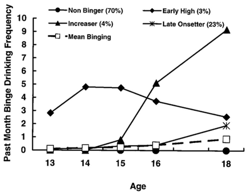
Mean binge drinking scores at each age for each trajectory group, with total sample mean scores.
Figure 1 shows the observed trajectories for the four groups. We labeled these trajectory groups as follows: Non-bingers (70%); Early Highs (3%); Increasers (4%); and Late Onsetters (23%). Note that the trajectory that we labeled as Early Highs begins to show a decline in late adolescence. In fact, when we extended these trajectories into young adulthood (age 21), most of the Early Highs matured out of binge drinking; thus, this trajectory more accurately reflects a group whose binge drinking was limited to adolescence. (These data are not shown here, but are available from the first author upon request.) Note also that the averaged total sample trajectory (mean binge drinking) shows a slight, steady increase in binge drinking frequency through adolescence, a pattern that does not adequately capture the various developmental trajectories actually occurring during this period.
Although this analysis found somewhat similar general patterns in binge drinking trajectories from ages 13 to 18 as Schulenberg et al. (1996) (none, rare, chronic, decreased, increased, and fling), and Muthén and Shedden (1999) (norm, up and high), it is important to note that those latter studies examined binge drinking trajectories from ages 18 to 24. The relationships between adolescent binge drinking trajectories found in this study (ages 13 to 18) and binge drinking patterns in young adulthood remain to be examined.
Individuals were next classified into the trajectory class with the highest posterior probability. This procedure makes the assumption that the error in classification made when placing a person in one and only one class based on the posterior probabilities is small and so does not bias the coefficient estimates nor the standard errors to an important degree. Muthén (Muthén, 2000; Muthén and Shedden, 1999) describes methods that may be used without this simplifying assumption. Table 2 provides the mean posterior probabilities conditional on class assignment for the four trajectory classes. Note that the average probabilities for the assigned groups are 97%, 96%, 92%, and 98% for the Nonbingers, Early Highs, Increasers, and Late Onsetters, respectively, indicating reasonably low classification error.
Table 2.
Average Binge Trajectory Assignment Probability, Conditional on Assignment by Maximum Probability Rule
| Assigned Group
|
|||||
|---|---|---|---|---|---|
| Probability conditional on group membership | Nonbingers | Early Highs | Increasers | Late Onsetters | |
| Nonbingers | 97% | 0% | 0% | 0% | |
| Early Highs | 0% | 96% | 1% | 1% | |
| Increasers | 0% | 1% | 92% | 1% | |
| Late Onsetters | 3% | 2% | 6% | 98% | |
|
| |||||
| TOTAL | 100% | 100% | 100% | 100% | |
Significant Group Differences in Elementary School and Adolescence
We conducted χ2 analyses to determine if groups differed in terms of demographics and control variables when they were in the fifth and sixth grades. To represent the concept of risk exposure, these demographic and control variables were dichotomized where 1 represented being in the highest quartile of risk on that predictor, and 0 represented the remainder. Table 3 shows the observed prevalences and significant differences for the four trajectory groups.
Table 3.
Prevalences of Demographics and Control Variables for the Four Binge Trajectory Groups
| Nonbingers | Early Highs | Increasers | Late Onsetters | χ2 (df = 3) | p | |
|---|---|---|---|---|---|---|
| Age 10–12 y | ||||||
| Male | 47% | 50% | 71% | 61% | 15.7 | 0.001 |
| SESa | 26% | 35% | 16% | 19% | 6.7 | 0.081 |
| Internalizingb | 28% | 42% | 23% | 25% | 3.6 | 0.308 |
| Externalizingb | 21% | 50% | 35% | 25% | 13.4 | 0.004 |
| Delinquencyb | 21% | 53% | 33% | 34% | 19.1 | 0.001 |
| Alcohol useb | 19% | 46% | 33% | 27% | 16.7 | 0.001 |
| Drug useb | 20% | 56% | 17% | 31% | 25.3 | 0.001 |
| Educationa | 24% | 39% | 29% | 24% | 3.4 | 0.340 |
| Prosocial involvementa | 26% | 23% | 32% | 20% | 4.1 | 0.249 |
| Family bondinga | 24% | 27% | 16% | 28% | 2.2 | 0.532 |
| Age 13–18 y
|
13% | 69% | 77% | 49% | 197.0 | 0.000 |
| Average drug use in adolescenceb | ||||||
lowest quartile;
highest quartile. SES, socioeconomic status.
The binge drinking trajectories were significantly different by gender [χ2(3) = 15.7, p < 0.001], with more males in the Increasers and Late Onset groups than in the other two groups. Although not statistically significant [χ2(3) = 6.7, ns], the Early Highs had the largest number of low SES subjects of all groups. The Early Highs also had the highest prevalences of extreme Externalizing [χ2(3) = 13.4, p < 0.004] and Internalizing [χ2(3) = 3.6, ns], although the latter was not statistically significant. The trajectory groups were significantly different in early problem behaviors, with the Early Highs being highest in prevalence of early frequent delinquency [χ2(3) = 19.1, p < 0.001], alcohol use [χ2(3) = 16.7, p < 0.001], and drug use [χ2(3) = 25.3, p < 0.001]. The trajectory groups were not significantly different in the prosocial control variables of academic performance [χ2(3) = 3.4, NS], prosocial involvement [χ2(3) = 4.1, NS], or family bonding [χ2(3) = 2.2, NS]. Thus, although binge drinking behavior was not measured until the seventh grade, there were large differences between the Early High bingers and their peers in terms of early problem behaviors as early as the fifth and sixth grades. The groups also differed significantly from each other in terms of their drug use during adolescence [χ2(3) = 197.0, p < 0.001]. The Increasers and the Early Highs had higher prevalences of frequent drug use than the Late Onsetters and Nonbingers.
Significant Group Differences in Young Adult Outcomes
Table 4 provides a summary of the trajectory group differences for each age 21 outcome. For this analysis we also performed χ2 analyses. Significant differences in binge drinking trajectories were found for crime [χ2(3) = 15.8, p < 0.001], alcohol abuse/dependence [χ2(3) = 80.1, p < 0.001], drug abuse/dependence [χ2(3) = 20.8, p < 0.001], high school completion [χ2(3) = 48.1, p < 0.001], involvement in clubs/activities [χ2(3) = 12.2, p < 0.007], and family bonding [χ2(3) = 13.0, p < 0.005]. Group differences in productive engagement [χ2(3) = 5.3, NS] and depression [χ2(3) = 2.5, NS] were not statistically significant. Overall, the Early Highs had the poorest outcome profile in terms of prosocial functioning at age 21. They had the lowest levels of high school completion, involvement in prosocial activities, and family bonding. In terms of negative outcomes, the Increasers, not the Early Highs, had the highest prevalences of crime and alcohol and drug abuse/dependence at age 21. For all outcome main effects, the adolescent Nonbingers had the highest prevalence of prosocial and lowest prevalence of antisocial outcomes at age 21.
Table 4.
Prevalences of Age 21 Outcome Variables for the Four Binge Trajectory Groups
| Nonbingers | Early Highs | Increasers | Late Onsetters | χ2 (df = 3) | p | |
|---|---|---|---|---|---|---|
| Depression | 13% | 21% | 17% | 17% | 2.5 | 0.484 |
| Crime | 27% | 54% | 43% | 39% | 15.8 | 0.001 |
| Alcohol abuse/dependence | 7% | 13% | 43% | 30% | 80.1 | 0.001 |
| Drug abuse/dependence | 4% | 13% | 17% | 13% | 20.8 | 0.001 |
| High school completion | 92% | 63% | 80% | 76% | 48.1 | 0.001 |
| Engagement in school or working | 85% | 73% | 74% | 83% | 5.3 | 0.150 |
| Involvement in clubs/activities | 58% | 25% | 43% | 53% | 12.2 | 0.007 |
| Family bonding | 67% | 33% | 57% | 67% | 13.0 | 0.005 |
Logistic Regressions Predicting Age 21 Outcomes
For the combined person- and variable-centered portion of our analysis, we then conducted three-step hierarchical logistic regression analyses to examine how well the trajectory groups predicted each young adult outcome, once childhood measures and adolescent drug use were considered. In step 1 we entered only gender, SES, and the proxy control variable from grades five and six. In step 2 we entered three dummy variables for the Increasers, Early Highs and Late Onsetters versus the Nonbingers as the referent group. Finally, in step 3 we added the adolescent drug use variable to see if illicit drug use during adolescence would eliminate the significance of binge drinking in predicting outcomes in early adulthood. Table 5 shows the odds ratios for the hierarchical logistic regressions predicting the negative outcomes, and Table 6 shows those for the positive outcomes. In addition, Tables 5 and 6 present the change in the −2 log likelihood for each step, and its significance and change in degrees of freedom.
Table 5.
Odds Ratios for Hierarchical Logistic Regression Models Predicting Negative Outcomes at Age 21
| Major Depression | Crime | Alcohol Abuse/Dependence | Drug Abuse/Dependence
|
|||||||||
|---|---|---|---|---|---|---|---|---|---|---|---|---|
| Step | 1 | 2 | 3 | 1 | 2 | 3 | 1 | 2 | 3 | 1 | 2 | 3 |
| Gender (male) | .67 | .66 | .66 | 2.20* | 2.18* | 2.19* | 3.30* | 2.83* | 2.81* | 2.63* | 2.28* | 2.24* |
| SES | 1.02 | 1.01 | 1.01 | 1.05 | 1.00 | 1.00 | 1.19 | 1.09 | 1.11 | 1.22 | 1.17 | 1.20 |
| Control variable† | .60‡
1.20 |
.66
1.05 |
.69
.94 |
2.24* | 2.08* | 1.96* | 1.22 | 1.12 | 1.09 | 1.26 | 1.17 | 1.11 |
| Early Higha | 1.89 | 1.49 | 2.03 | 1.58 | 1.34 | 1.06 | 3.04 | 1.61 | ||||
| Increasera | 1.81 | 1.37 | .93 | .69 | 7.71* | 5.53* | 3.84* | 1.62 | ||||
| Late Onsettera | 1.35 | 1.19 | 1.54* | 1.36 | 5.34* | 4.72* | 2.90* | 2.08* | ||||
| Adolescent | 1.21 | 1.26 | 1.23 | 1.64* | ||||||||
| Overall −2 log | 566.6 | 728.1* | 578.9* | 377.0* | ||||||||
| Likelihood Δ −2 log | 3.1 | 2.1 | 5.5 | 3.7 | 55.3* | 2.7 | 14.1* | 13.1* | ||||
| Likelihood Degrees of freedom | 4 | 3 | 1 | 3 | 3 | 1 | 3 | 3 | 1 | 3 | 3 | 1 |
p < 0.05; SES, socioeconomic status.
The control variable is a proxy of the age 21 outcome assessed in 5th and 6th grade.
For major depression, there were two proxy control variables: internalizing and externalizing, respectively.
Reference category is nonbinger.
Table 6.
Odds Ratios for Hierarchical Logistic Regression Models Predicting Positive Outcomes at Age 21
| Completed High School
|
Productive Involvement
|
Involvement in Clubs/Activities
|
Parental Bonding
|
|||||||||
|---|---|---|---|---|---|---|---|---|---|---|---|---|
| Step | 1 | 2 | 3 | 1 | 2 | 3 | 1 | 2 | 3 | 1 | 2 | 3 |
| Gender (male) | .51* | .57* | .57* | .77 | .80 | .81 | 1.21 | 1.28 | 1.30 | 1.03 | 1.05 | 1.07 |
| SES | 1.58* | 1.84* | 1.83* | 1.73* | 1.77* | 1.76* | 1.31* | 1.31* | 1.31* | 1.62* | 1.61* | 1.60* |
| Control variable† | 3.20* | 3.03* | 3.01* | 1.70* | 1.65* | 1.64* | 1.40* | 1.44* | 1.46* | 1.46* | 1.45* | 1.42* |
| Early Higha | .16* | .21* | .57 | .74 | .24* | .31* | .27* | .38* | ||||
| Increasera | .35* | .47 | .49 | .64 | .45* | .61 | .57 | .93 | ||||
| Late Onsettera | .22* | .24* | .77 | .87 | .73 | .84 | .91 | 1.11 | ||||
| Adolescent Drug Use | .83 | .84 | .80* | .72* | ||||||||
| Overall −2 log | 507.8* | 700.3* | 1032.8* | 959.9* | ||||||||
| Likelihood Δ −2 log | 39.2* | 1.9 | 3.9 | 2.2 | 15.3* | 4.8* | 10.9* | 9.7* | ||||
| Likelihood Δ df for model | 3 | 3 | 1 | 3 | 3 | 1 | 3 | 3 | 1 | 3 | 3 | 1 |
p < .05; SES, socioeconomic status.
The control variable is a proxy of the age 21 outcome assessed in 5th and 6th grade.
Reference category is nonbinger.
As with the outcome prevalence patterns discussed earlier, binge drinking patterns in adolescence significantly predicted crime, alcohol abuse/dependence, drug abuse/dependence, high school completion, involvement in clubs and activities, and parental bonding at age 21. They did not significantly predict depression or productive involvement at age 21 in the logistic regression analyses (Step 2 in Tables 5 and 6). The addition of drug use significantly improved the model fit above binge drinking for drug abuse/dependence, prosocial involvement, and parental bonding (Step 3 in Tables 5 and 6). However, even after controlling for drug use, adolescent binge drinking patterns continued to predict these outcomes.
Early Highs
Interestingly, once gender, SES, and the early proxy measure were controlled, the Early Highs were not more likely than the Nonbingers to be depressed, involved in crime, or alcohol- or drug-dependent at age 21 (Table 5). However, even once these measures and adolescent drug use were controlled, the Early Highs were less likely than the Nonbingers to complete high school, be involved in clubs and activities, and be bonded to their parents at age 21 (Table 6). Thus, Early High binge drinking appears to inhibit positive development by age 21, but does not appear to contribute independently to negative outcomes in early adulthood beyond the contribution of early involvement in these behaviors. The only significant negative outcome observed for Early Highs in the main effects model was for criminal behavior, and that variable was no longer significant once early delinquency was controlled.
Increasers
In agreement with the group prevalences discussed earlier, Table 5 shows that the Increasers had the highest likelihood of alcohol abuse or dependence at age 21, and that this difference remained significant after controlling for gender, SES, early drinking, and adolescent drug use. The Increasers also were more likely than Non-bingers to be drug-dependent at age 21; this difference was no longer significant; however, once adolescent drug use was controlled. Table 6 shows that the Increasers were less likely than Nonbingers to complete high school and to be involved in clubs and activities at age 21, but these differences disappeared after controlling for adolescent drug use. For this group, their increasing pattern of binge drinking through adolescence is, perhaps, a marker for future alcohol problems; they may be on a path to alcohol abuse and dependence. However, it is their adolescent drug use, not their trajectory of binge drinking, that predicts negative outcomes other than alcohol abuse and dependence by age 21. Note that, while the Increasers did have a delayed increase in binge drinking frequency relative to the Early Highs, they attained substantially higher levels of binge drinking frequency at age 18 than any of the other groups attained at any time point from age 13 to 18. This rapidly increasing frequency of binge drinking through age 18 may be consistent with the more pervasive problem profile exhibited by the Increasers in early adulthood.
Late Onsetters
Finally, the Late Onsetters were more likely than Nonbingers to be alcohol- and drug-dependent and involved in crime. These differences remained significant even after controlling for gender, SES, and the early proxy measures (Table 5). This effect remained for alcohol and drug dependence after controlling for adolescent drug use; however, the relationship dropped to non-significance for crime involvement at age 21. Table 6 shows that the Late Onsetters also were less likely than Nonbingers to complete high school, a difference that remained after controlling for adolescent drug use.
DISCUSSION
Adolescent binge drinking is related significantly to both prosocial and antisocial outcomes at age 21, even after controlling for gender, SES, early proxy measures, and adolescent drug use. However, the effects depend on the particular pattern or trajectory of binge drinking. For example, Early High binge drinking predicted poor prosocial functioning in adulthood, but had no significant effect on negative outcomes independent of the subjects’ earlier problem behavior. Compared to Nonbingers, Early Highs were at a greater risk for not graduating from high school, for not being involved in prosocial activities, and for having low bonding to their parents even after controlling for gender, SES, early proxy measures, and adolescent drug use. This finding is consistent with the social development model (Catalano and Hawkins, 1996), which hypothesizes that early antisocial behavior interferes with the development of prosocial protective factors at the next life stage. Table 4 shows this group had higher rates of crime, alcohol abuse and dependence, and drug abuse and dependence at age 21 than Nonbingers; however, Early High binging did not appear to contribute independently to problem behaviors in early adulthood. Thus, for this group Early High binging may be part of a cluster of problem behaviors resulting in fewer positive and more negative outcomes in young adulthood.
On the other hand, the Increasing binge drinkers, who became the highest-level binge drinkers at the end of adolescence (and in fact into adulthood), were at greatest risk for alcohol and drug abuse or dependence and at high risk for not completing high school and not being involved in clubs and activities. However, consistent with Kandel et al.’s findings (1986), Increasers were not at greater risk for these outcomes (with the exception of alcohol abuse/dependence) when drug use was added to the model. The Increasers also had the highest rates of drug use during adolescence; thus, their drug use was more likely a contributing factor to many of their problems in young adulthood than was their binge drinking behavior. Their pattern of binge drinking in adolescence did, however, increase their risk for alcohol abuse and dependence by age 21 independent of drug use.
Those who began binge drinking in late adolescence (Late Onsetters) were at increased risk for not completing high school and for all the negative outcomes except depression and crime when compared to Nonbingers, even after controlling for their adolescent drug use. Thus, the effects of adolescent binge drinking clearly depend on the developmental stage within which it occurs, and the developmental course it follows.
These effects of specific patterns of binge drinking in adolescence would not have been detected readily employing variable-centered analyses alone, and they clarify some inconsistencies in the literature. For example, using a variable-centered approach (structural equation modeling), Newcomb and Bentler (1988) found some positive and some negative consequences of adolescent alcohol use. Using a latent growth modeling approach, which did not attend to group differences in growth, Duncan et al. (1997) found largely negative outcomes of adolescent alcohol use. The differences between the findings of these two studies may be due in part to the fact that differences in developmental trajectories were masked by the two approaches. In the present study the person-centered analysis provided more information on the specific patterns of binge drinking that are related to positive and negative outcomes. High-level binge drinking in early adolescence interfered with the achievement of prosocial outcomes in adulthood. On the other hand, higher levels of binge drinking in late adolescence (Increasers and Late Onsetters) predicted negative outcomes in young adulthood.
The finding of developmentally distinct binge drinking trajectories has implications for research and prevention practice. These findings suggest that researchers should consider the possibility that the behavior under study is heterogeneously developmental. Examining problem behaviors, such as alcohol use, drug use, or crime, from a variable-centered approach risks masking important developmental differences among youths. An important next step in this research is to identify differential predictors of membership in these trajectories. Studies of delinquency (Bartusch et al., 1997; Farrington and Hawkins, 1991) suggest that the predictors of early-onset delinquency may differ from predictors of delinquency that begins in adolescence. Identifying differential predictors of these binge drinking trajectories would inform the development of prevention programs aimed at reducing binge drinking and consequent problems in early adulthood.
Acknowledgments
The authors acknowledge Marsha Bates, Kathy Bucholz, Kristina Jackson, Bengt Muthén, Robert Abbott, and Daniel Nagin for their helpful feedback on this manuscript.
Footnotes
An earlier version of this paper was presented at the Annual Meeting of the Research Society on Alcoholism, June 26–July 1, 1999, Santa Barbara, CA.
Supported by grants from the National Institute on Alcohol Abuse and Alcoholism (#R21AA10989–01), National Institute on Drug Abuse (#DA/AA 03995 and #R01DA09679), and the Robert Wood Johnson Foundation (#031925).
References
- Achenbach TM. Integrative Guide for the 1991 CBCL/4–18:YSR, and TRF Profiles. University of Vermont, Department of Psychiatry; Burlington, VT: 1991. [Google Scholar]
- American Psychiatric Association. Diagnostic and Statistical Manual of Mental Disorders. 4. American Psychiatric Association; Washington, DC: 1994. [Google Scholar]
- Anthony JC, Warner LA, Kessler RC. Comparative epidemiology of dependence on tobacco, alcohol, controlled substances, and inhalants: Basic findings from the National Comorbidity Survey. In: Marlatt GA, VandenBos GR, editors. Addictive Behaviors: Readings on Etiology, Prevention, and Treatment. American Psychological Association; Washington, DC: 1997. pp. 3–39. [Google Scholar]
- Bartusch DRJ, Lynam DR, Moffitt TE, Silva PA. Is age important? Testing a general versus developmental theory of antisocial behavior. Criminology. 1997;35:13–48. [Google Scholar]
- Bates ME. Integrating person-centered and variable-centered approaches to the study of developmental courses and transitions in alcohol use: Introduction to the Special Section. Alcohol Clin Exp Res. 2000;24:878–881. [PubMed] [Google Scholar]
- Bates ME. Psychology Recent Dev Alcohol. 1993;11:45–72. [PubMed] [Google Scholar]
- Bell R, Wechsler H, Johnston LD. Correlates of college student marijuana use: Results of a US national survey. Addiction. 1997;92:571–581. [PubMed] [Google Scholar]
- Bryk AS, Raudenbush SW. Hierarchical Linear Models: Applications and Data Analysis Methods. Sage; Thousand Oaks, CA: 1992. [Google Scholar]
- Cairns RB. Phenomena lost: Issues in the study of development. In: Valsiner J, editor. Individual Subject and Scientific Psychology. Perseus Books; Cambridge: 1986. pp. 97–112. [Google Scholar]
- Catalano RF, Hawkins JD. The social development model: A theory of antisocial behavior. In: Hawkins JD, editor. Delinquency and Crime: Current Theories. Cambridge University Press; New York: 1996. pp. 149–197. [Google Scholar]
- Clausen JS. Adolescent competence and the shaping of the life course. Am J Sociol. 1991;96:805–842. [Google Scholar]
- Duncan SC, Alpert A, Duncan TE, Hops H. Adolescent alcohol use development and young adult outcomes. Drug Alcohol Depend. 1997;49:39–48. doi: 10.1016/s0376-8716(97)00137-3. [DOI] [PubMed] [Google Scholar]
- Duncan SC, Duncan TE. A multivariate latent growth curve analysis of adolescent substance use. Structural Equation Modeling. 1996;3:323–347. [Google Scholar]
- Erikson EH. The Life Cycle Completed. WW Norton & Company; New York: 1982. [Google Scholar]
- Farrington DP, Hawkins JD. Predicting participation, early onset, and later persistence in officially recorded offending. Criminal Behav Ment Health. 1991;1:1–33. [Google Scholar]
- Fergusson DM, Lynskey MT. Alcohol misuse and adolescent sexual behaviors and risk taking. Pediatrics. 1996;98:91–96. [PubMed] [Google Scholar]
- Johnston LD, O’Malley PM, Bachman JG. National Survey Results on Drug Use From the Monitoring the Future Study 1975–1997. US Department of Health and Human Services; Rockville, MD: 1998. [Google Scholar]
- Jones BL, Nagin DS, Roeder K. A SAS Procedure Based on Mixture Models for Estimating Developmental Trajectories. 1999 Technical report retrieved October 25, 1999 from the World Wide Web: http://www.stat.cmu.edu/cmu-stats/tr/tr684/tr684.html.
- Jones BL. [Accessed October 25, 1999];National Consortium on Violence Research SAS Proc TRAJ Home. 1999 World Wide Web: http://www.stat.cmu.edu/~bjones/traj.html.
- Kandel DB, Davies M, Karus D, Yamaguchi K. The consequences in young adulthood of adolescent drug involvement. Youth Society. 1986;21:441–445. doi: 10.1001/archpsyc.1986.01800080032005. [DOI] [PubMed] [Google Scholar]
- Kandel DB. Drug and drinking behavior among youth. Am Sociol Rev. 1980;6:235–285. [Google Scholar]
- Kass RE, Raftery AE. Bayes factor. J Am Stat Assoc. 1995;90:773–795. [Google Scholar]
- Labouvie EW, Pandina RJ, Johnson V. Developmental trajectories of substance use in adolescence: Differences and predictors. Int J Behav Dev. 1991;14:305–328. [Google Scholar]
- Magnussen D, Bergman LR. Individual and variable-based approaches to longitudinal research on early risk factors. In: Rutter M, editor. Studies in Psychosocial Risk: The Power of Longitudinal Data. Cambridge University Press; New York: 1988. pp. 45–46. [Google Scholar]
- Muthén B, Muthén L. The development of heavy drinking and alcohol-related problems from ages 18 to 37 in a U.S. national sample. J Stud Alcohol. 2000;61:290–300. doi: 10.15288/jsa.2000.61.290. [DOI] [PubMed] [Google Scholar]
- Muthén BO, Shedden K. Finite mixture modeling with mixture outcomes using the EM algorithm. Biometrics. 1999;55:463–469. doi: 10.1111/j.0006-341x.1999.00463.x. [DOI] [PubMed] [Google Scholar]
- Muthén B, Muthén LK. Integrating person-centered and variable-centered analysis: Growth mixture modeling with latent trajectory classes. Alcohol Clin Exp Res. 2000;24:882–891. [PubMed] [Google Scholar]
- Nagin DS. Analyzing developmental trajectories: A semiparametric, group-based approach. Psychol Methods. 1999;4:139–157. doi: 10.1037/1082-989x.6.1.18. [DOI] [PubMed] [Google Scholar]
- Nagin DS, Land K. Age, criminal careers, and population heterogeneity: Specification and estimation of a nonparametric, mixed Poisson model. Criminology. 1993;31:327–362. [Google Scholar]
- Nagin DS, Tremblay RE. Trajectories of boys’ physical aggression, opposition, and hyperactivity on the path to physically violent and nonviolent juvenile delinquency. Child Dev. 1999;70:1181–1196. doi: 10.1111/1467-8624.00086. [DOI] [PubMed] [Google Scholar]
- National Highway Traffic Safety Administration (NHTSA) 1995 Youth Fatal Crash and Alcohol Facts. NHTSA, U.S. Dept. of Transportation; Washington, DC.: 1997. [Google Scholar]
- Nelson CB, Heath AC, Kessler RC. Temporal progression of alcohol dependence symptoms in the U.S. household population: Results from the National Comorbidity Survey. J Consult Clin Psychol. 1998;66:474–483. doi: 10.1037//0022-006x.66.3.474. [DOI] [PubMed] [Google Scholar]
- Newcomb MD, Bentler PM. Consequences of Adolescent Drug Use: Impact on the Lives of Young Adults. Sage Publications; New York: 1988. [Google Scholar]
- Quigley LA, Marlatt AG. Drinking among young adults: Prevalence, patterns and consequences. Alcohol Health Res World. 1996;20:185–191. [PMC free article] [PubMed] [Google Scholar]
- Raftery AE. Bayesian model selection in social research. Sociological Methodology. 1995;25:111–164. [Google Scholar]
- Robins LN, Helzer JE, Croughan J, Williams JBW, Spitzer RL. NIMH Diagnostic Interview Schedule: Version III. National Institute of Mental Health; Rockville, MD: 1981. [Google Scholar]
- Schulenberg J, O’Malley PM, Bachman JG, Wadsworth KN, Johnston LD. Getting drunk and growing up: Trajectories of frequent binge drinking during the transition to young adulthood. J Stud Alcohol. 1996;57:289–304. doi: 10.15288/jsa.1996.57.289. [DOI] [PubMed] [Google Scholar]
- Smart RG. Behavioral and social consequences related to the consumption of different beverage types. J Stud Alcohol. 1996;57:77–84. doi: 10.15288/jsa.1996.57.77. [DOI] [PubMed] [Google Scholar]
- Thakker KD. An overview of health risks and benefits of alcohol consumption. Alcohol Clin Exp Res. 1998;22(Suppl):285.S–298S. doi: 10.1097/00000374-199807001-00003. [DOI] [PubMed] [Google Scholar]
- Vaillant GE. The Natural History of Alcoholism: Causes, Patterns, and Paths to Recovery. Harvard University Press; Cambridge, MA: 1983. [Google Scholar]
- White HR, Bates ME, Labouvie E. Adult outcomes of adolescent drug use: A comparison of process-oriented and incremental analyses. In: Jessor R, editor. New Perspectives on Adolescent Risk Behavior. Cambridge University Press; New York: 1998. pp. 150–181. [Google Scholar]
- White HR. Longitudinal stability and dimensional structure of problem drinking in adolescence. J Stud Alcohol. 1987;48:541–550. doi: 10.15288/jsa.1987.48.541. [DOI] [PubMed] [Google Scholar]
- Willett JB, Sayer AG. Using covariance structure analysis to detect correlates and predictors of individual change over time. Psychol Bull. 1994;116:363–381. [Google Scholar]
- Zucker RA. Developmental aspects of drinking through the young adult years. In: Blane HT, Chaftez ME, editors. Youth, Alcohol and Social Policy. Plenum Press; New York: 1979. [Google Scholar]
- Zucker RA. Pathways to alcohol problems and alcoholism: A developmental account of the evidence for multiple alcoholisms and for contextual contributions to risk. In: Zucker RA, Howard J, Boyd GM, editors. The Development of Alcohol Problems: Exploring the Biopsychosocial Matrix of Risk. National Institute on Alcohol Abuse and Alcoholism Research Monograph No. 26. National Institute on Alcohol Abuse and Alcoholism; Rockville, MD: 1994. pp. 255–289. [Google Scholar]
- Zucker RA. The four alcoholisms: A developmental account of the etiologic process. In: Rivers PC, editor. Nebraska Symposium on Motivation 1986: Alcohol and Addictive Behavior. University of Nebraska Press; Lincoln, NE: 1987. [PubMed] [Google Scholar]