Dynamical signatures of cellular fluctuations and oscillator stability in peripheral circadian clocks

Abstract

Cell-autonomous and self-sustained molecular oscillators drive circadian behavior and physiology in mammals. From rhythms recorded in cultured fibroblasts we identified the dominant cause for amplitude reduction as desynchronization of self-sustained oscillators. Here, we propose a general framework for quantifying luminescence signals from biochemical oscillators, both in populations and individual cells. Our model combines three essential aspects of circadian clocks: the stability of the limit cycle, fluctuations, and intercellular coupling. From population recordings we can simultaneously estimate the stiffness of individual frequencies, the period dispersion, and the interaction strength. Consistent with previous work, coupling is found to be weak and insufficient to synchronize cells. Moreover, we find that frequency fluctuations remain correlated for longer than one clock cycle, which is confirmed from individual cell recordings. Using genetic models for circadian clocks, we show that this reflects the stability properties of the underlying circadian limit-cycle oscillators, and we identify biochemical parameters that influence oscillator stability in mammals. Our study thus points to stabilizing mechanisms that dampen fluctuations to maintain accurate timing in peripheral circadian oscillators.

Introduction

Cell-autonomous molecular pacemakers coordinated by pacemaker neurons in the suprachiasmatic nucleus (SCN) drive circadian rhythms in mammals (Reppert and Weaver, 2002; Schibler and Sassone-Corsi, 2002). Whereas central pacemakers were shown to elicit robust circadian firing rhythms with negligible damping (Welsh et al, 1995; Liu et al, 1997), oscillations of mRNA levels in peripheral organs and cell cultures showed marked damping (Yamazaki et al, 2000; Yoo et al, 2004). This raised the question whether SCN oscillations were qualitatively different from those in peripheral tissues, even though the underlying molecular clocks seem to utilize the same genetic components (Yagita et al, 2001; Schibler and Sassone-Corsi, 2002).

Several studies using luciferase and GFP reporters have now clarified the issue. For instance, tissue explants generate robust oscillatory bioluminescence signals that damp out after ∼7 days, whereas rhythms in cultured cells derived from the same tissues persist for ∼20 days (Yoo et al, 2004). Repeating the experiment in SCN lesioned mice does not abolish rhythms but induces phase shifts, indicating the existence of organ-specific synchronization cues probably masked by the SCN under normal conditions. Although this suggested that peripheral clocks can tick independent of a functional SCN, the issue was addressed directly in a series of studies that combined single cells and population assays. Recordings in immortalized (Nagoshi et al, 2004) and primary (Welsh et al, 2004) mouse fibroblasts showed that single cells generated cell-autonomous rhythms. Furthermore, the effect of a serum shock was to resynchronize randomly phased oscillators rather than jumpstarting arrested oscillators (Nagoshi et al, 2004). Mathematical analysis of longer bioluminescence recordings reinforced these observations and confirmed that dephasing was the dominant cause for amplitude reduction. In embryonic cell lines from the zebrafish that were transfected with a zfperiod4-luciferase reporter, Carr and Whitmore (2005) observed the resynchronization of single cellular oscillators by light. Importantly, by monitoring individual cells during 6 days, the authors observed that successive periods within a single cell drift in time (Supplementary Figure S2). Consensus from several models thus strongly supports that damping seen in cultures at the population level reflects desynchronization rather than damping of individual oscillators. Moreover, the default unsynchronized state of a cell population consists of individual oscillating cells with random phase distributions so that populations appear globally non-oscillating. Serum pulses merely resynchronize the phases without starting new oscillations. Finally, all referred work hypothesized that interoscillator coupling was absent in cell cultures, a result that was consistent with relatively short coculture experiments (Nagoshi et al, 2004) and also found in cyanobacterial colonies (Mihalcescu et al, 2004). Nevertheless, the relevance of intercell interaction in peripheral clocks remains open.

Here, we present a general methodology to study biomolecular oscillators and deduce informative parameters from population recordings or individual cells. We investigate the combined effects of limit-cycle stability, intrinsic cellular fluctuations, and oscillator coupling using a compact stochastic mathematical model. Specifically we study the consequences of noisy frequencies and phase coupling on the collective phase dynamics in populations of peripheral circadian oscillators. Using two independent bioluminescence data sets from Nagoshi et al (2004) and Welsh et al (2004), we show that our low-dimensional model captures the data nicely. Our formulation also allows estimating the intercellular coupling strength; we find that whereas the coupling strength is insufficient for synchronization, phase crosstalk between cells can occur at a low rate. Furthermore, we predict a new time scale of about 1 day describing the stiffness of individual circadian frequencies, a quantity that also directly probes the stability of the autonomous oscillator. Finally, we identify biochemical parameters that influence oscillator stability in two models of mammalian circadian clocks.

Results and discussion

Model for interacting noisy-phase oscillators

Because they contain a low number of relevant parameters, phase oscillators have been useful to study collective synchronization, phase shifting, and entrainment properties of circadian oscillators (Winfree, 1967; Garcia-Ojalvo et al, 2004; Mihalcescu et al, 2004; Roenneberg et al, 2005). Our previous model for populations of phase oscillators assumed that each cell has a randomly chosen static frequency. In addition, each oscillator could damp out so that its peak-to-trough amplitude ratio would decrease exponentially with a time scale T. Using bioluminescence recordings from whole cell cultures, this study showed that the primary cause for amplitude loss was detuning owing to the frequency dispersion σ_f and not the decay of individual oscillators. This was indicated by the long decay time T (18.8 days) found to be comparable to the experiment duration (Nagoshi et al, 2004).

The frequency drifts reported by Carr and Whitmore (2005), together with our observation that the static frequency model underestimated the frequency dispersion measured in individual cells with a YFP reporter (Nagoshi et al, 2004), prompted us to extend our model to individual oscillator frequencies that drift in time. Additionally, we explicitly model intercellular coupling instead of assuming that it can be neglected. Briefly, the phase derivative for each cell is taken as a stochastic time-dependent frequency plus coupling term (Figure 1A). Specifically, the frequencies are modeled as an Ornstein–Uhlenbeck (OU) process. The latter is commonly used in the cellular context (Garcia-Ojalvo et al, 2004; Suel et al, 2006) where fluctuations are expected to be correlated in time owing to finite half-lives of other cell components. OU processes are the simplest generalization of Gaussian white noise that introduce exponentially decaying time correlations with a characteristic time scale γ (Figure 1B; for introduction see Lemons, 2002). Only few parameters are introduced. First σ_f, the frequency dispersion, is a measure of noise. More precisely, it describes how the limit cycle is susceptible to noise sources, for example, intrinsic noise. On the contrary, γ is a property of the deterministic system (when η=0 in Figure 1A), which reflects the stiffness of the frequencies or, more generally, the stability of the oscillator. By varying γ the model interpolates smoothly between static frequencies (small γ), whereas for larger γ the frequencies change rapidly and the phase dynamics resembles a diffusion process (Supplementary Figure S2), as in Mihalcescu et al (2004). The coupling among phases is described by the parameter K. With coupling (K>0), the model becomes far more complicated, but assuming all-to-all coupling, we derived an expression for the critical coupling value K_c above which the population synchronizes (Rougemont and Naef, 2006). The behavior of the synchronization threshold is recapitulated in Supplementary Figure S3, and reflects that rapidly drifting frequencies are easier to synchronize than stiff frequencies.

Figure 1.

Stochastic phase model with drifting frequencies and intercellular phase coupling. (A) An extended Kuramoto model for the oscillator phases φ_i(t) and frequencies f_i(t) describes coupled circadian phase oscillators. The total luminescence signal s(t) is the sum of a population of initially N₀ oscillators each contributing a cosine signal centered around a constant A with relative amplitude B. Cell death follows a Poisson process with time constant τ reflected by the indicator variable θ_i^τ(t) taking value 1 before (and 0 after) cell i has died. The time-dependent frequencies and phases of the individual oscillators are subject to a stochastic differential equation (cf. Materials and methods and Supplementary information). (B) Sample frequency trajectory; γ and σ_f² are free constants representing the inverse memory of the frequency trajectories and the frequency dispersion, respectively. (C) Parameter listing. K describes the intercellular coupling between the phases and is taken as all-to-all. More realistic coupling geometries are considered in Figure 3.

Other fluctuations could influence the biolumiscence signals. For example, amplitude fluctuations have been considered by Mihalcescu et al (2004). However, these do not affect the estimation of the dephasing parameters γ and σ_f from population-averaged signals. Namely, if A_i(t) describes the time-dependent amplitude of cell i, we only need to assume that its fluctuations are independent of the time of cell death (described by the random variable θ_i^τ(t) in equation (2); Figure 1) and the phases ϕ_i(t). Moreover, a sufficiently large number of cells is required (cf. Supplementary information), which is verified empirically by the good fit in Figure 2A (inset). Moreover, we estimated that 5000 cells contribute to the signal at the end of the recording time (Nagoshi et al, 2004). The same arguments hold for fluctuations in the relative amplitude B. However, relative amplitude fluctuations play a role in the analysis of autocorrelation from single-cell recordings (Figure 2D).

Figure 2.

Analysis of bioluminescence data by Nagoshi et al (referred to as D1). (A) Raw data reproduced from Nagoshi et al (2004). Inset: logarithmic scale emphasizes the exponential signal decrease reflecting cell death with half-life 3.22 days. (B) Maximum likelihood fit of the detrended signal Z to our model. The data were detrended using band-pass filtering as detailed by Nagoshi et al (2004). (C) Posterior likelihoods of the parameters. Projections for each pair of model parameters γ, σ_f, and K are shown: red indicates high probability; standard errors around the maximum likelihood parameters are indicated (cf. Table I). The critical coupling lines (black) with fixed third parameter indicate that the coupling should be increased for synchrony (first two panels), or alternatively the frequency dispersion should be reduced (third panel). (D, E) Frequency drifts from bioluminescence signal in individual cells from the autocorrelation analysis of 10 individual cells (from Welsh et al, 2004, Figures 2B and 3C). (D) Each color is the autocorrelation for one cell. For convenience the absolute value is plotted and the maxima are fit to the envelope

predicted from the model (cf. panel E and Supplementary information) which leads to a best fit (black line) with C=0.72, σ_f=0.059±0.003 day⁻¹, and γ=0.39±0.11 day⁻¹. (E) A single cell was simulated for 30 days with parameters similar to those for the data D2 in Table I (γ=0.9 day⁻¹ and σ_f=0.1 day⁻¹). Amplitude fluctuations were modeled as a correlated process with mean B, γ_B=5γ, and σ_B/B=0.4, leading to a rapidly decreasing initial transient in the envelope (exact prediction in blue; cf. Supplementary information). The approximation for large γ_B used to fit panel A is shown is cyan. The short (dephasing) and long-time (phase diffusion) regimes are indicated in red and green, respectively.

Frequency dynamics in cell-autonomous oscillators

To establish whether the new model accurately describes bioluminescence signals, we analyzed two independent data sets (from Figure 3B in Nagoshi et al (2004) and Figure 3C, luminometer track in Welsh et al, 2004). Hereafter, we refer to theses data as D1 and D2, respectively. Both used cultured fibroblast cells; however, the first were from the immortalized NIH3T3 line, whereas the second were dissociated from tails of knock-in mPer2^{Luciferase−SV40} mice. The 19-day bioluminescence recording D1 (Figure 2A) uses a Bmal1 luceriferase reporter. To connect model and theory, we fit the detrended signal Z(t) to the predicted population-averaged signal (Figure 2B). Fitting the two data sets leads to nicely compatible values for the parameters σ_f and γ describing the individual oscillators (Figure 2B, Supplementary Figure S5 and Table I). Note that all parameters can be estimated reliably, and the error bars indicate that the model does not overfit the data. We discuss the results for D1 in some detail. The new model estimates a frequency dispersion of 0.1 per day, which converted to hours leads to a standard deviation in the periods of 2.4 hrs, which is very close to the 2.9 h measured in single cells (Nagoshi et al, 2004) and more accurate than the previous estimate (0.93 h) based on static frequencies. Furthermore, the estimated γ=0.64±0.17, reflecting a frequency damping time of 1.56 days, is consistent across data sets. This implies that frequency disturbances take longer than a period length to decay; in other words the initiation of a new cycle does not fully erase the previous cycle.

Figure 3.

Comparison of synchronization behavior between the all-to-all model and random 2D cell arrangements. (A) 2D cell culture geometries are modeled as random Voronoi tessellations of the square. First and second neighbors of the central cell (in yellow) are indicated in green and red, respectively. (B) Synchronization transition for cell cultures with local coupling. The synchronization parameter R_∞ is computed as a function of the coupling strength K for three different geometries: all-to-all coupling (red), nearest-neighbor coupling (blue), and coupling extending to second nearest neighbor (purple). For each coupling strength and geometry, 10 000 cells were simulated. Mean and standard error are represented for five independent cell arrangements (details in Supplementary information, section 4).

Table 1.

Parameter estimates in two independent data sets

	Half-life (days)	K (day−1)	B	Period 1/μf (h)	γ (day−1)	σf (day−1)
Nagoshi et al (D1)	3.22±0.01**	0.05±0.02*	0.90±0.01**	25.75±0.02**	0.64±0.17**	0.1±0.007**
Welsh et al (D2)	55.2±1.3**	0.02±0.08	0.26±0.003**	25.48±0.03**	0.89±0.64	0.1±0.01**

Nonlinear expression for the predicted Z(t) (cf. Supplementary information) was fit to the luminescence signals (Figure 2C and Supplementary Figure S5) to estimate K, B, γ, μ_f, and σ_f. Exponential trend (cell half-life) was estimated from the linear regression in Figure 2A (inset). ^* and ^** refer to fit parameters with P<0.01 and P<0.001, respectively. Standard errors in the parameter estimates are also indicated.

Whereas σ_f and γ are comparable in both data sets, the cell half-lives and oscillatory amplitude B differ significantly. For example, it appears that the primary cell cultures from D2 are longer lived, with an estimated decay significantly longer than the 3.2 days from D1. A probable explanation is that the primary culture was grown under much richer serum (10%) condition than the immortalized fibroblasts (0.5%), and this drastically affected cell lifespan (U Schibler, personal communication). On the other hand, the oscillatory amplitude is larger in D1 (B=0.9 versus 0.26). Here, it is likely that synthesis and degradation kinetics of the reporter transcript and protein play a role, as these clearly determine circadian amplitude. For example, the protein half-life of a rhythmically transcribed gene must be short enough for rhythmic protein accumulation to be detected. It is possible that the mRNA half-life of the fusion protein in the mPer2^{Luciferase−SV40} mouse is longer than in the Bmal-luciferase reporter (Figure 2B). For instance, the mRNA amplitudes reported by Gachon et al (2004) (Figure 1D and F) in the liver are approximately 5–fold for per2 and 10-fold for Bmal1, which is similar to our estimates, but the stability of the luciferase fusion gene should be predominantly determined by the luciferase 3′UTR rather than the per2 3′UTR.

Oscillators exchange subthreshold phase signals

Our approach also allows to estimate intercell coupling. Previous work addressed the phase coupling among bacterial colonies using a model for two coupled phase oscillators (Mihalcescu et al, 2004); here we use our recent result for coupling in oscillator populations (Rougemont and Naef, 2006). From D1 and D2, we find that the coupling strength is subthreshold and therefore cannot synchronize the cells, consistent with previous coculture (Nagoshi et al, 2004) and transplantation experiments (Guo et al, 2006). How could this small phase crosstalk be mediated in cell cultures? Whereas coupling in SCN neurons depends on synaptic transmission (Liu and Reppert, 2000; Yamaguchi et al, 2003; Ohta et al, 2005; Maywood et al, 2006), coupling in peripheral circadian clocks could occur via paracrine signaling, for example, a broad class of signaling cues were shown to elicit circadian rhythms in fibroblasts (Balsalobre et al, 2000a, 2000b). It is possible that some residual form of such cues could be active in culture. The measured coupling (K=0.05 day⁻¹) signifies that neighboring cells are able to shift the phase of an oscillator by half a cycle in 10 days. In comparison, synchrony would develop if the same delay could be mediated in less than about 5 days, assuming fixed σ_f and γ (Figure 2C, left). Alternatively, synchrony would occur if the stiffness was reduced (γ increased) or the frequency dispersion was reduced by about twofold (Figure 2C, right).

In the calculations presented so far, we have assumed that each cell was evenly coupled to every other cell (all-to-all coupling). This choice reflected mathematical convenience, as we can then derive expressions for the critical coupling strength. To investigate the validity of this approximation, we assume that synchrony is mediated through diffusing peptides. With sizes of about 1 nm, we can estimate using the Einstein–Stokes formula that 10 cell shells can be reached within 12 min, which is small compared with the oscillatory period. Therefore, if signaling peptides are secreted, each cell effectively receives temporally coherent synchronization signals from a large number of neighboring cells. To assess whether this is sufficient for synchronization, we have assumed realistic cell geometries generated from random Voronoi tilings (Figure 3A). In these, each cell has an average of six neighbors, but the environment for each cell is slightly different. Simulations show that adding cell shells leads to a synchronization behavior that converges to the all-to-all model (Figure 3B), indicating that our estimates of coupling are reliable. In fact the coupling estimated from the all-to-all model is a lower bound for the real coupling strength.

Frequency dynamics from individual cell recordings

Next we analyze the frequency dynamics in single-cell luciferase recordings (cf. Figures 2B and 3C in Welsh et al, 2004) using autocorrelation of the signals. A property of autocorrelations is that these are unaffected by coupling as long as K is below the synchronization threshold (section 1.5, Supplementary information). This highlights an interesting difference between single cell and population recordings: subthreshold coupling cannot be estimated from single cells, whereas it can be estimated from the dephasing dynamics of initially synchronized populations, as in Figure 2C. One salient feature of individual cell bioluminescence signals is that their amplitude fluctuates significantly. The short time behavior of autocorrelations shows abrupt drop in the autocorrelation within the first period (arrow in Figure 2D), which is captured by a simple model, assuming independent amplitude and phase fluctuations (Figure 2E and Supplementary information, section 1.3). Even though we had few cells at our disposal, fitting the mode to the data leads to an estimated frequency dispersion σ_f within a factor two of the population estimate, whereas the drift parameter γ is within the error bars of the population estimate. This good agreement (cf. overlay in Supplementary Figure S6) from different approaches thus supports that correlated frequency fluctuations are an essential signature of peripheral circadian oscillators.

Origins of frequency fluctuations

Phase models, which have been popular in circadian biology since the work of Winfree (1967), postulate that molecular mechanisms generate sustained oscillations without describing the molecular interactions among clock components. However, the wealth of biochemical data about circadian pathways has allowed the development of rate equation models that show how limit-cycle oscillation can arise (Forger and Peskin, 2003; Leloup and Goldbeter, 2003; Locke et al, 2005) and resist noise in clock circuits (Barkai and Leibler, 2000; Gonze et al, 2002; Vilar et al, 2002; Forger and Peskin, 2005; Gonze and Goldbeter, 2006). Several of these models rely on the mutual feedback of an activator and repressor pair that triggers relaxation oscillations (Barkai and Leibler, 2000; Vilar et al, 2002), whereas others use delayed feedback (Gonze et al, 2002). Under physiological conditions, such chemical reaction networks face two types of fluctuations: (i) those that follow from the finite numbers of molecules, DNA, mRNA, or proteins (often termed intrinsic) and (ii) fluctuations that act globally on all parts of the network like thermal fluctuations or changes in cell volume in dividing cells (termed extrinsic).

Recent stochastic simulations probing the role of intrinsic noise in two mammalian clock models showed that the period variability is directly affected by the number of clock proteins. Specifically, the variance in circadian period length is inversely proportional to the number of molecules (Leloup and Goldbeter, 2003; Forger and Peskin, 2005). Whereas intrinsic fluctuations thus lead to period variability, the magnitude of these fluctuations depends on the stability of the deterministic limit cycle. This is reflected in our phase model by the relation σ_f²=σ_η²/(2γ), that is, for fixed noise σ_η², more stable limit cycles (γ large) are less susceptible to noise and thus have smaller frequency dispersion. As γ measures the stability of the phase oscillator, it is natural to ask how this inverse timescale relates to a canonical measure of limit-cycle stability, namely the negative logarithm of the leading Floquet multiplier μ_F (Eckmann and Ruelle, 1985; Strogatz, 2000). In Supplementary Figures S7–S9, we use γ_F=−log(μ_F) to measure limit-cycle stability. To address the above question we apply Floquet analysis to a generic circadian model describing a delayed negative feedback loop (Gonze and Goldbeter, 2006). This model includes three dynamical variables and describes mRNA transcription, translation, and nuclear translocation of an autoregulatory clock protein. In parallel we simulate intrinsic noise through a master equation and use the Gillespie (1976) algorithm to simulate trajectories (as in Gonze and Goldbeter, 2006) from which we estimate the variability in frequency. By varying the number of molecules (Ω) and transcription rate, we found that population averages of stochastic trajectories could be well approximated by the form predicted for the phase model (Supplementary Figure S9), with parameter values γ=γ_F and σ_f very close to the estimate from the trajectories. This correspondence shows that the Floquet stability can be probed experimentally using our method, and that we can use powerful analytical tools to study how limit-cycle stability depends on model parameters. For illustration, we vary each of the nine parameters independently while monitoring stability and period of the limit cycle (Supplementary Figure S7). We find that stability can be increased most efficiently by raising the transcription rate (v_s) of the mRNA or by reducing the half-max parameter (K_m) for mRNA degradation. Meanwhile, increasing the translation rate of the protein (k_s) or the nuclear translocation rate (k₁) reduces period length as expected, whereas period lengthens with increased v_s.

Finally, we apply stability analysis to a detailed sixteen-dimensional model for the mammalian circadian clock (Leloup and Goldbeter, 2003). In the mammalian clock, the principal activators are the Bmal1, Clock, and Npas2 transcription factors, whereas repression is mediated by Per1, Per2, Cry1, Cry2, and RevErbα (Schibler and Naef, 2005). The model by Leloup and Goldbeter (2003) (LG) is based on a merged Per gene, a merged Cry, and Bmal1. It also describes protein phosphorylation, for example, Per is phosphorylated by casein kinase 1 (CK1), complex formation, and transport from the cytoplasm to nucleus where mRNAs are transcribed. The model has 53 parameters, but we restricted ourselves to four groups of parameters: transcription rates, phosphorylation rates of the Per and Cry proteins, complex formation between Per and Cry, and nuclear translocation rates (Supplementary Figure S8). Sensitivity analysis for the period length in this model was detailed by Leloup and Goldbeter (2004). Among the changes that most affect period length, increased complex formation rate and nuclear entry rate shorten the period as expected, whereas increased Bmal1 transcription or Period phosphorylation lengthens the period (Supplementary Figure S8). Floquet analysis shows that only few of the parameters tested strongly influence limit-cycle stability, and most of the changes lead to less stable oscillators. Note that the value of γ_F (0.87 inverse periods) for the nominal parameters are in the range of our measured γ (Table I), suggesting that the LG model has realistic limit-cycle stability properties. In contrast, the above three-variable model has a more stable limit cycle with γ_F=2.65 inverse periods. Interestingly, the parameter that most increases the stability is the phosphorylation rate of Per (Supplementary Figure S8, star). Thus, this predicts that within the LG model, the observed frequency dispersion could be reduced maximally by overexpressing CK1 such that the phosphorylation rate of Per would be increased by a factor of 3.

Conclusion and outlook

We showed how circadian bioluminescence signals recorded in peripheral clock cells can be analyzed to provide insight into three essential aspects of circadian clocks: limit-cycle stability, their susceptibility to fluctuations, and intercellular coupling. Analyzing independent bioluminescence recordings leads to consistent parameter for frequency dispersion, frequency stiffness, and coupling between cells. Furthermore, estimates from populations and single cells were in good agreement. Interestingly, our study predicted that oscillator stability is such that frequencies in individual cells remain correlated beyond one circadian cycle length. Additionally, we estimated phase crosstalk in cell cultures, which indicated that the coupling strength was nonzero but only about half of that needed to synchronize the cells. We showed that collective synchronization would occur if the frequency dispersion would be tighter, for example, if it could be reduced by a factor of about 2 (Figure 2C). One possible role of residual but subthreshold coupling in peripheral circadian oscillators is that it facilitates entrainment by systemic cues, which are restricted to time windows shorter than the period (supported by simulations, data not shown). Thus, our phase model shows how dynamical stability, cellular noise level, and intercellular coupling shape collective and individual bioluminescence rhythms in peripheral circadian oscillators. We ended by linking the stability of limit cycles to the properties of biochemical oscillator models and pointed toward molecular mechanisms that are predicted to increase the stability of the circadian clock in mammals.

Biochemical oscillators commonly serve to coordinate cellular processes occurring over a wide range of timescales. We showed that peripheral circadian oscillators are weakly coupled, but others interact strongly to elicit collective synchronization. The latter include the respiratory cycle in yeast grown under constant condition (Henson, 2004; Klevecz et al, 2004; Locke et al, 2005) or the somite clock, as measured in tissue explants (Horikawa et al, 2006; Masamizu et al, 2006). The approach presented here is naturally suited to study fluctuations in these collectively synchronized biological timekeepers. As luminescence reporters are becoming widely used in chronobiology, we expect that it will provide a compact framework to compare the dephasing dynamics in a broad class of molecularly distinct oscillators operating in fluctuating cellular environments.

Materials and methods

Data sets

We analyze two independent circadian bioluminescence data sets (from Figure 3B in Nagoshi et al (2004) and Figure 3C, luminometer track in Welsh et al (2004)). We refer to these data as D1 and D2, respectively.

Phase model

Drifting frequencies with the properties of a fixed mean E[f]=μ and variance var[f]=σ_f² are generated through an Ornstein–Uhlenbeck process described by the stochastic differential equation

in which η(t) is a Gaussian white noise source with variance parameterized as σ_η²=2γσ_f². Here, γ and σ_f² are free constants representing the decay rate and amplitude of frequency fluctuations, respectively. The mathematical aspects of synchronization in this model are found in Rougemont and Naef (2006). Additional results used in this paper, for example, the form for the autocorrelations, are derived from Supplementary information.

Simulations were performed with the discrete dynamical updates (Lemons, 2002):

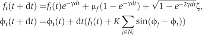where N_i denotes the neighbors of cell i and ζ is a random number drawn from a Gaussian distribution with mean 0 and variance σ_f². Initial conditions φ_i(t=0)=0 reflect synchronization by the serum pulse and f_i(t=0) was drawn for a Gaussian with mean μ_f and variance σ_f². For Figure 2B and C, the number of oscillators (N=5000) was sufficient to prevent finite size effects from influencing parameter estimation in the time span from 0 to 10 days.

Regression and detrending

To study the effects of phase dynamics, we work with the detrended variable

which renormalizes the signal for cell death and amplitude A (Nagoshi et al (2004); Supplementary information). N(t) denotes the population size at time t and Z(t) lies between −1 and +1.

All regression and associated statistical tests were performed with the R language for statistical computing and graphics (http://cran.r-project.org) using the lm and nlm routines. Simulations were implemented in R and C. For the parameter estimations in Table I, a routine, that simulated the averaged signal from N=5000 oscillators was passed to the nlm routine to fit the detrended signal Z(t). Posterior likelihoods of the parameters in Figure 2 were generated using a grid of parameters in the (K, γ), (K, σ_f), (γ, σ_f) planes that were passed to the same simulation routine.

Voronoi tilings

Voronoi tilings for randomly seeded cell nuclei were used to define neighbors in 2D cell arrangements. First and second neighbors were considered for the coupling term in Figure 3. Details about the geometrical algorithm are given in Section 4 of Supplementary information.

Floquet analysis

We compute the Floquet multipliers for the Gonze and Leloup models using the continuation software AUTO (Doedel et al, 2001). To find the limit cycles, initial transcription rates were set to zero, for which the trivial fixed point with all concentrations equal to 0 is stable. Parameters were then increased one by one to their nominal values (those used in the original articles) whereas limit cycles solutions were tracked along with their periods and Floquet multipliers.

Supplementary Material

Supplementary Information

References

- Balsalobre A, Brown SA, Marcacci L, Tronche F, Kellendonk C, Reichardt HM, Schutz G, Schibler U (2000a) Resetting of circadian time in peripheral tissues by glucocorticoid signaling. Science 289: 2344–2347 [DOI] [PubMed] [Google Scholar]
- Balsalobre A, Marcacci L, Schibler U (2000b) Multiple signaling pathways elicit circadian gene expression in cultured Rat-1 fibroblasts. Curr Biol 10: 1291–1294 [DOI] [PubMed] [Google Scholar]
- Barkai N, Leibler S (2000) Circadian clocks limited by noise. Nature 403: 267–268 [DOI] [PubMed] [Google Scholar]
- Carr AJ, Whitmore D (2005) Imaging of single light-responsive clock cells reveals fluctuating free-running periods. Nat Cell Biol 7: 319–321 [DOI] [PubMed] [Google Scholar]
- Doedel EJ, Paffenroth RC, Chapneys AR, Fairgrieve TF, Kutzetsov YA, Oldman BE, Sandstede B, Wang XJ (2001) AUTO2000: continuation and bifurcation software for ordinary differential equations. Technical Report, California Institute of Technology, 2001
- Eckmann JP, Ruelle D (1985) Ergodic theory of chaos and strange attractors. Rev Mod Phys 57: 617–656 [Google Scholar]
- Forger DB, Peskin CS (2003) A detailed predictive model of the mammalian circadian clock. Proc Natl Acad Sci USA 100: 14806–14811 [DOI] [PMC free article] [PubMed] [Google Scholar]
- Forger DB, Peskin CS (2005) Stochastic simulation of the mammalian circadian clock. Proc Natl Acad Sci USA 102: 321–324 [DOI] [PMC free article] [PubMed] [Google Scholar]
- Gachon F, Fonjallaz P, Damiola F, Gos P, Kodama T, Zakany J, Duboule D, Petit B, Tafti M, Schibler U (2004) The loss of circadian PAR bZip transcription factors results in epilepsy. Genes Dev 18: 1397–1412 [DOI] [PMC free article] [PubMed] [Google Scholar]
- Garcia-Ojalvo J, Elowitz MB, Strogatz SH (2004) Modeling a synthetic multicellular clock: repressilators coupled by quorum sensing. Proc Natl Acad Sci USA 101: 10955–10960 [DOI] [PMC free article] [PubMed] [Google Scholar]
- Gillespie DT (1976) Exact stochastic simulation of coupled chemical reactions. J Phys Chem 81: 2340–2361 [Google Scholar]
- Gonze D, Goldbeter A (2006) Circadian rhythms and molecular noise. Chaos 16: 026110. [DOI] [PubMed] [Google Scholar]
- Gonze D, Halloy J, Goldbeter A (2002) Robustness of circadian rhythms with respect to molecular noise. Proc Natl Acad Sci USA 99: 673–678 [DOI] [PMC free article] [PubMed] [Google Scholar]
- Guo H, Brewer JM, Lehman MN, Bittman EL (2006) Suprachiasmatic regulation of circadian rhythms of gene expression in hamster peripheral organs: effects of transplanting the pacemaker. J Neurosci 26: 6406–6412 [DOI] [PMC free article] [PubMed] [Google Scholar]
- Henson MA (2004) Modeling the synchronization of yeast respiratory oscillations. J Theor Biol 231: 443–458 [DOI] [PubMed] [Google Scholar]
- Horikawa K, Ishimatsu K, Yoshimoto E, Kondo S, Takeda H (2006) Noise-resistant and synchronized oscillation of the segmentation clock. Nature 441: 719–723 [DOI] [PubMed] [Google Scholar]
- Klevecz RR, Bolen J, Forrest G, Murray DB (2004) A genomewide oscillation in transcription gates DNA replication and cell cycle. Proc Natl Acad Sci USA 101: 1200–1205 [DOI] [PMC free article] [PubMed] [Google Scholar]
- Leloup JC, Goldbeter A (2003) Toward a detailed computational model for the mammalian circadian clock. Proc Natl Acad Sci USA 100: 7051–7056 [DOI] [PMC free article] [PubMed] [Google Scholar]
- Leloup JC, Goldbeter A (2004) Modeling the mammalian circadian clock: sensitivity analysis and multiplicity of oscillatory mechanisms. J Theor Biol 230: 541–562 [DOI] [PubMed] [Google Scholar]
- Lemons DS (2002) An Introduction to Stochastic Processes in Physics. Baltimore and London: The Johns Hopkins University Press [Google Scholar]
- Liu C, Reppert SM (2000) GABA synchronizes cloack cells within the suprachiasmatic circadian clock. Neuron 25: 123–128 [DOI] [PubMed] [Google Scholar]
- Liu C, Weaver DR, Strogatz SH, Reppert SM (1997) Cellular construction of a circadian clock: period determination in the suprachiasmatic nuclei. Cell 91: 855–860 [DOI] [PubMed] [Google Scholar]
- Locke JC, Millar AJ, Turner MS (2005) Modelling genetic networks with noisy and varied experimental data: the circadian clock in Arabidopsis thaliana. J Theor Biol 234: 383–393 [DOI] [PubMed] [Google Scholar]
- Masamizu Y, Ohtsuka T, Takashima Y, Nagahara H, Takenaka Y, Yoshikawa K, Okamura H, Kageyama R (2006) Real-time imaging of the somite segmentation clock: revelation of unstable oscillators in the individual presomitic mesoderm cells. Proc Natl Acad Sci USA 103: 1313–1318 [DOI] [PMC free article] [PubMed] [Google Scholar]
- Maywood ES, Reddy AB, Wong GK, O'Neill JS, O'Brien JA, McMahon DG, Harmar AJ, Okamura H, Hastings MH (2006) Synchronization and maintenance of timekeeping in suprachiasmatic circadian clock cells by neuropeptidergic signaling. Curr Biol 16: 599–605 [DOI] [PubMed] [Google Scholar]
- Mihalcescu I, Hsing W, Leibler S (2004) Resilient circadian oscillator revealed in individual cyanobacteria. Nature 430: 81–85 [DOI] [PubMed] [Google Scholar]
- Nagoshi E, Saini C, Bauer C, Laroche T, Naef F, Schibler U (2004) Circadian gene expression in individual fibroblasts: cell-autonomous and self-sustained oscillators pass time to daughter cells. Cell 119: 693–705 [DOI] [PubMed] [Google Scholar]
- Ohta H, Yamazaki S, McMahon DG (2005) Constant light desynchronizes mammalian clock neurons. Nat Neurosci 8: 267–269 [DOI] [PubMed] [Google Scholar]
- Reppert SM, Weaver DR (2002) Coordination of circadian timing in mammals. Nature 418: 935–941 [DOI] [PubMed] [Google Scholar]
- Roenneberg T, Dragovic Z, Merrow M (2005) Demasking biological oscillators: properties and principles of entrainment exemplified by the Neurospora circadian clock. Proc Natl Acad Sci USA 102: 7742–7747 [DOI] [PMC free article] [PubMed] [Google Scholar]
- Rougemont J, Naef F (2006) Collective synchronization in populations of globally coupled phase oscillators with drifting frequencies. Phys Rev E Stat Nonlin Soft Matter Phys 73: 011104. [DOI] [PubMed] [Google Scholar]
- Schibler U, Naef F (2005) Cellular oscillators: rhythmic gene expression and metabolism. Curr Opin Cell Biol 17: 223–229 [DOI] [PubMed] [Google Scholar]
- Schibler U, Sassone-Corsi P (2002) A web of circadian pacemakers. Cell 111: 919–922 [DOI] [PubMed] [Google Scholar]
- Strogatz S (2000) Nonlinear Dynamics and Chaos, with Applications to Physics, Biology, Chemistry and Engineering. Cambridge, MA: Perseus Books [Google Scholar]
- Suel GM, Garcia-Ojalvo J, Liberman LM, Elowitz MB (2006) An excitable gene regulatory circuit induces transient cellular differentiation. Nature 440: 545–550 [DOI] [PubMed] [Google Scholar]
- Vilar JM, Kueh HY, Barkai N, Leibler S (2002) Mechanisms of noise-resistance in genetic oscillators. Proc Natl Acad Sci USA 99: 5988–5992 [DOI] [PMC free article] [PubMed] [Google Scholar]
- Welsh DK, Logothetis DE, Meister M, Reppert SM (1995) Individual neurons dissociated from rat suprachiasmatic nucleus express independently phased circadian firing rhythms. Neuron 14: 697–706 [DOI] [PubMed] [Google Scholar]
- Welsh DK, Yoo SH, Liu AC, Takahashi JS, Kay SA (2004) Bioluminescence imaging of individual fibroblasts reveals persistent, independently phased circadian rhythms of clock gene expression. Curr Biol 14: 2289–2295 [DOI] [PMC free article] [PubMed] [Google Scholar]
- Winfree AT (1967) Biological rhythms and the behavior of populations of coupled oscillators. J Theor Biol 16: 15–42 [DOI] [PubMed] [Google Scholar]
- Yagita K, Tamanini F, van Der Horst GT, Okamura H (2001) Molecular mechanisms of the biological clock in cultured fibroblasts. Science 292: 278–281 [DOI] [PubMed] [Google Scholar]
- Yamaguchi S, Isejima H, Matsuo T, Okura R, Yagita K, Kobayashi M, Okamura H (2003) Synchronization of cellular clocks in the suprachiasmatic nucleus. Science 302: 1408–1412 [DOI] [PubMed] [Google Scholar]
- Yamazaki S, Numano R, Abe M, Hida A, Takahashi R, Ueda M, Block GD, Sakaki Y, Menaker M, Tei H (2000) Resetting central and peripheral circadian oscillators in transgenic rats. Science 288: 682–685 [DOI] [PubMed] [Google Scholar]
- Yoo SH, Yamazaki S, Lowrey PL, Shimomura K, Ko CH, Buhr ED, Siepka SM, Hong HK, Oh WJ, Yoo OJ, Menaker M, Takahashi JS (2004) PERIOD2∷LUCIFERASE real-time reporting of circadian dynamics reveals persistent circadian oscillations in mouse peripheral tissues. Proc Natl Acad Sci USA 101: 5339–5346 [DOI] [PMC free article] [PubMed] [Google Scholar]
Associated Data
This section collects any data citations, data availability statements, or supplementary materials included in this article.
Supplementary Materials