A dense array stimulator to generate arbitrary spatio-temporal tactile stimuli

Abstract

The generation and presentation of tactile stimuli presents a unique challenge. Unlike vision and audition, in which standard equipment such as monitors and audio systems can be used for most experiments, tactile stimuli and/or stimulators often have to be tailor-made for a given study. Here, we present a novel tactile stimulator designed to present arbitrary spatio-temporal stimuli to the skin. The stimulator consists of 400 pins, arrayed over a 1 cm² area, each under independent computer control. The dense array allows for an unprecedented number of stimuli to be presented within an experimental session (e.g., up to 1200 stimuli per minute) and for stimuli to be generated adaptively. The stimulator can be used in a variety of modes and can deliver indented and scanned patterns as well as stimuli defined by mathematical spatio-temporal functions (e.g., drifting sinusoids). We describe the hardware and software of the system, and discuss previous and prospective applications.

1. Introduction

The generation and presentation of tactile stimuli presents a unique challenge. Unlike vision and audition, in which standard equipment such as monitors and audio systems can be used for most experiments, tactile stimuli and/or stimulators often have to be tailor-made for a given study. We have developed a novel tactile stimulator designed to present arbitrary spatio-temporal stimuli to the skin (see Pawluk et al., 1998 for a description of the prototype). This tactile display consists of 400 tactors – linear motors – arranged in four planes of 100 motors each (Fig. 1). The planes are stacked one on top of another and mounted such that the shafts from each motor converge at a point 48.5 cm below the lowest plane. The shafts consist of a series of stainless steel tubes that are reduced in diameter from the motor to the point of contact with the skin. The contactors are presently configured in a 20 × 20 matrix, 1 cm × 1 cm, but this configuration can be easily modified. Each motor is individually controlled and has a dynamic range from 0 Hz (DC displacement) to over 250 Hz. Vertical displacements can be generated in the range of 2000 μm at 0 Hz to 100 μm at 250 Hz. Patterns generated on the array can be updated every 1 ms. The need for such a display has been recognized for a number of years.

Fig. 1.

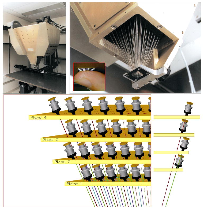
Top left panel: View of the dense array stimulator mounted on the 3-axis stage. Top right panel: Bottom view of the 400-probe stimulator with every fourth pin included to show the internal structure. Inset: Close-up of a finger pressed up against the array. Bottom panels: Layout of the four planes of motors.

With this 400-probe array, complex spatio-temporal patterns are being presented to the skin of both human observers, in psychophysical studies, and to monkeys, in both psychophysical and neurophysiological studies. This array permits us to generate complex spatio-temporal patterns that simulate the kind of stimulation generated by a finger coming in contact with surfaces. The idea behind the design was to create a display that matched or exceeded the skin’s mechanoreceptive capabilities. There are two key components to the display: the motors and associated hardware that generate the mechanical stimuli, and the software and associated hardware, that produce and store the signals that drive the motors. Together, these components permit the generation of spatio-temporal patterns at rates up to 1200 patterns per minute (assuming a typical duration of 50 ms per stimulus). The present paper presents a description of the system as it exists today, hardware and software, its capabilities, as well as some sample results obtained with the device.

1.1. Background

The design of the 400-probe stimulator was based on what is known about the neuroanatomical, neurophysiological, and psychophysical characteristics of the tactile system. In particular, the stimulator was designed to be used on the glabrous skin of the hand. It is among the most sensitive areas of the body, and has been the site of practically all of the studies of mechanoreception in human and non-human primates. Results from neuroanatomical and neurophysiological studies with humans and non-human primates are in agreement that there are at least three types of mechanoreceptive afferents. Humans appear to have a fourth type not found in non-human primates (Johnson et al., 2000; Johnson, 2001). The classification of these four types of afferents is based on the size of their receptive fields, small versus large, and their response to sustained stimulation, slow versus fast adapting. The four types are slowly adapting type 1 (SA1) afferents, which have small receptive fields and produce sustained responses to static indentations; rapidly adapting (RA) afferents, which, like their SA1 counterparts, have small receptive fields but produce transient responses at the onset and offset of indentations; Pacinian (PC) fibers, which also produce transient responses to indentations but have large receptive fields; and slowly adapting type 2 (SA2) fibers, which produce sustained responses to sustained skin stretch and have large receptive fields. There is considerable evidence that, of the four types of primary afferents, SA1 and RA fibers are most sensitive to spatial patterns, and of the two, SA1 afferents appear to convey the finest spatial information (Johnson and Hsiao, 1992).

Because one of the main aims in the development of the 400-probe array was to assess spatial aspects of mechanoreception, we were particularly concerned with the neuroanatomical and neurophysiological responses of SA1 and RA fibers. The density of innervation of the two types of receptors associated with these afferents leads to estimated mean spacing between receptive field centers of about 0.82 mm for RA and 1.0 mm for SA1 mechanoreceptors (Johnson et al., 2000). Results from psychophysical measures of spatial sensitivity are consistent with these estimates of innervation density (Johnson and Phillips, 1981; Phillips and Johnson, 1981). The spatial resolution of the 400-probe stimulator was designed to exceed that of the somatosensory periphery: the center-to-center spacing of the tactors was 0.5 mm.

Furthermore, the temporal response profile of the stimulator was approximately matched to that of mechanoreceptive afferent fibers. SA1 and RA fibers respond best to lower frequencies, 80 Hz and below. When the response of PC fibers is taken into consideration, the mechanoreceptive system responds to stimuli ranging in frequency from 0 Hz (static stimuli) to about 300 Hz (Mountcastle et al., 1972). Thus, the tactors were designed to deliver vibratory stimuli at frequencies up to 250 Hz or more.

1.2. Previous devices

Several devices have been used to present complex spatial patterns to the skin. The rotating drum (Johnson and Phillips, 1988) has been used to scan various types of raised patterns across the glabrous skin of both monkeys (Connor et al., 1990; Connor and Johnson, 1992; Blake et al., 1997; DiCarlo et al., 1998; DiCarlo and Johnson, 1999, 2000, 2002; Yoshioka et al., 2001), in neurophysiological experiments, and humans in psychophysical and percutaneous recording experiments (Phillips et al., 1992, 1990). Stimuli such as raised letters and textured surfaces are mounted on a drum; the drum is brought in contact with the skin and rotated. By moving the drum in small increments laterally, a spatial pattern can be moved across the fingerpad while single-unit recordings are made. Recordings of both peripheral (Connor et al., 1990; Connor and Johnson, 1992; Blake et al., 1997; Yoshioka et al., 2001) and central (Phillips et al., 1988; DiCarlo et al., 1998; DiCarlo and Johnson, 1999, 2002) neurons have been made with this device. The same spatial patterns can be presented to human observers in psychophysical tasks in which they are asked to identify the patterns. By varying the size and relative spacing of the elements in a pattern, and thus the spatial frequencies contained within that pattern, it can be shown which primary afferents are capable of responding to high spatial frequencies. This technique has helped establish the key role played by the SA1 system in the processing of fine spatial information.

The drum is very effective in simulating lateral movements of spatial patterns across the skin; however, there are some limitations to the system. Although there are known differences in the way that primary afferents respond to different temporal frequencies, these are not easily manipulated by the drum stimulator. On the other hand, the 400-probe stimulator can present spatial patterns at different temporal frequencies, as described below. Also, the rate at which patterns can be presented via the drum is somewhat limited while the dense array can deliver patterns at a high rate, typically 10–20 stimuli per second. In addition, the size of the drum limits the type and number of patterns that can be readily presented during an experimental session, as all of the patterns must fit along the circumference of the drum, while the dense array presents no such limitation. Finally, and perhaps most importantly, the stimulus patterns used on the drum need to be developed in advance. The patterns cannot be dynamically changed within a session based on neural or psychophysical responses.

Another device that has been that has been used in psychophysical and neurophysiological studies of spatial processing is the Optacon, a reading machine for the blind (Bliss et al., 1970). The display consists of 144 tactors arranged in a 6-column by 24-row array. The tactors generate vibratory patterns, approximately 230 pulses per second (pps). Although useful for generating temporal patterns, the tactor spacing is somewhat coarse, 1.1 mm center-to-center spacing between rows and 2.1 mm between columns. Furthermore, the display is limited in that the pulse rate is restricted to frequencies around 230 pps and can produce only small vertical displacements while exerting very little force. As a result, the array stimulates RA and PC fibers but not SA1 fibers (Gardner and Palmer, 1989), the receptor system important for encoding fine spatial features.

The device presently most similar to the 400-probe stimulator was developed by Summers and colleagues. The device consists of a 10 × 10 array of independently addressable tactors and uses bimorphs to generate vibrations. The contactors are arranged in a 1 cm² matrix and have a center-to-center spacing of 1 mm. The array can deliver vibratory frequencies between 20 and 400 Hz. The maximum displacement was reported to be 50 μm peak-to-peak at 40 Hz and 6 μm at 320 Hz (Summers and Chanter, 2002).

A somewhat different tack in generating tactile patterns was taken in a study investigating subjects’ ability to discriminate between sinusoidal gratings. In this study, the gratings, which differed in either amplitude or spatial frequency or both, were machined out of stainless steel bars. One indication of the difficulties in carrying out such a study and the need for a dense array is that the investigators estimated approximately 1000 h were required simply to make the gratings for the study (Nefs et al., 2001).

The remainder of the paper is divided into three sections. In the first section, we describe the hardware involved in delivering the stimuli and controlling the stimulator; in the second section, we describe the software that is used to drive the stimulator, to measure actual pin movements, and to link the stimulator to the data collection system; in the final section, we describe some applications of the stimulator to illustrate its versatility. Readers less interested in the technical aspects of the stimulator may wish to skip to this final section entitled “Applications.”

2. Hardware

2.1. Motor description

The linear motors were designed to have a 2–3 mm range of motion, a frequency response from DC to 300 Hz, and a large spring constant to reduce the effects of skin loading. Each linear motor contains two flat, helical springs upon which the moving magnet/shaft assembly is suspended (Fig. 2). The springs were etched from copper–beryllium sheets 0.13-mm thick and have a combined spring constant of 0.306 N/mm. When the skin is indented over an area approximately equivalent to that of 300 probes, the measured skin stiffness is 3.5 N/mm (Pawluk and Howe, 1999). Thus, the springs of the motors are approximately 25 times stiffer than the skin (91.8 N/mm for 300 probes versus 3.5 N/mm for an equivalent area of skin). The magnet is a high-energy permanent magnet (Dexter Permag Corporation, Karin, LA). Additional pole pieces and the inner shell, machined from a soft iron–cobalt (Hyperco, Logansport, IN), complete the magnetic circuit. The magnet, pole pieces, and spacers are mounted on a brass shaft and held in place by the optical target.

Fig. 2.

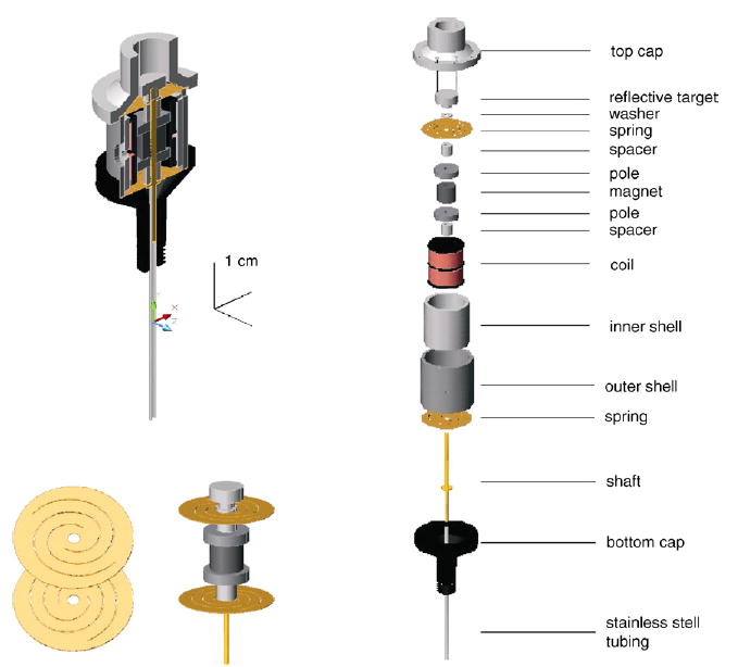
Top left panel: Illustration of a 400-probe motor cut in half lengthwise to reveal the internal structure. Bottom left panel: Close-up of the custom-made spring (left) and of the moving mass (right). Right panel: Diagram of the motor components.

Motion is achieved by applying voltage/current to the coil assembly that surrounds the magnet/pole assembly. The coil assembly is a continuous #38 copper wire wound around an anodized aluminum bobbin. The bobbin and winding pattern separate the wire into two distinct coils. The coil assembly is secured inside the inner shell with a single setscrew. The inner shell is then held inside the outer shell by another setscrew. The moving magnet/shaft assembly contacts the stationary shell assembly at the ends of the outer shell where the spring edges are secured by the top and bottom caps. The bottom cap is machined from plastic and has male threads to mount the motor into the dense array chassis. The top cap is machined from aluminum and holds the optical sensor and coil terminals. The sloped profile of the end caps prevents over-extension and deformation of the helical springs. Three screws clamp the top cap to the bottom cap and secure the moving shaft assembly.

Fig. 3 shows a typical frequency response for the linear motor. As the moving mass is approximately 12 g, the resonant frequency of the motor is around 35 Hz. Note that the range of motion is 3 mm although the maximum amplitude drops sharply at frequencies greater than 35 Hz. The maximal achievable frequency is constrained by the timing of the electronics more than it is by the frequency response of the motors, however. As commands are updated at a rate of 1000 Hz (see below), the maximal achievable frequency is 500 Hz, although the reliability of the sinusoids drops after 100 Hz (at which each stimulus cycle comprises 10 command cycles). Fig. 4 shows the fidelity of sinusoidal waveforms for frequencies ranging from 5 to 100 Hz.

Fig. 3.

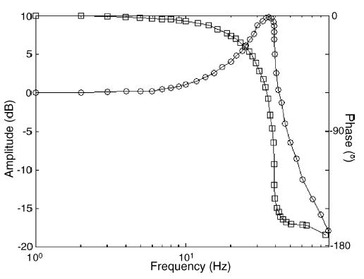
Frequency-response of a typical 400-probe motor. The peak-to-peak amplitude (circles) and relative phase (squares) of the motor response changes as a function of frequency when the sinusoidal command voltage is of constant amplitude.

Fig. 4.

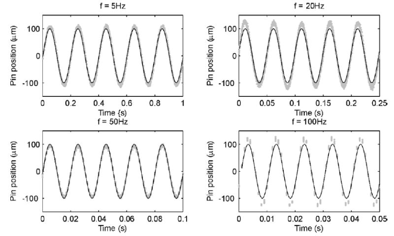
Five cycles of a sinusoidal stimulus at four frequencies (5, 10, 50 and 100 Hz) illustrating the fidelity of the waveform over this frequency range. The gray dots indicate the actual trajectory, the trace the desired trajectory. Ten repeats of the motor response are shown in each plot to highlight its repeatability. The differing density of samples across frequencies reflects the rate at which motor positions were sampled, namely 1000 Hz.

Linear displacement is transferred to the skin by a series of three concentric, telescoping stainless steel tubes terminating in a solid, 300-μm pin. The first and largest diameter tube is fixed to the brass shaft with epoxy. The next two tubes are glued (with epoxy) to each other. The solid stainless steel pin that contacts the skin is fixed with epoxy to the third tube. This assembly is secured inside the first tube using paraffin wax. The wax creates a remarkably strong and stable union while providing a means to adjust the overall shaft length by simply heating the shaft or shafts with hot air. The middle tube contains a 1-in. section of PEEK (polyetheretherketone; Upchurch Scientific, Inc., Oak Harbor, WA) plastic that blocks the transmission of any induced or capacitive currents to the skin.

Position sensing is achieved by an optical sensor (OP707, Optek, Carrollton, TX) encased in a light-tight, light-absorbent housing mounted on the rear of the motor. This sensor consists of an LED and a phototransistor in a 5-mm diameter cylindrical package. The LED illuminates a 6.5-mm diameter non-spectral reflective target mounted on the rear of the shaft, and the phototransistor, which has a sensitivity of approximately 1 V/mm, converts reflected light to current. The amount of light reflected to the detector varies non-linearly with the motion of the reflector, resulting in the detector voltage–displacement relationship shown in Fig. 5. The detector bandwidth is a function of the detector’s load resistance. The LED current for a given detector’s load resistance is adjusted to position the dynamic range around the desired operating point. Increasing the LED current tends to increase the dynamic range of the sensor, but at the cost of thermal stability.

Fig. 5.

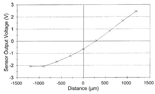
Sensor output as a function of the distance traveled by the pin.

2.1.1. Motor and sensor calibration

The relationship between the voltage input to each of the 400 pin motor amplifiers and their resulting real-world displacement is initially unknown. We calibrated each motor individually using a laser interferometer (Optodyne LDS 1000, Compton, CA), capable of measuring absolute displacement to sub-micron resolutions. Each motor was individually moved through a series of steps during the calibrating procedure. At every step, pin displacement was measured along with the corresponding motor voltage input. For each pin, the displacement data were fit to the voltage input values using a cubic polynomial. While calibrating motor input voltage, we simultaneously measured the sensor output and calibrated it to the same laser displacement data. The sensor voltage output of each motor was fit to the laser displacement data using another set of 400 cubic polynomials (Fig. 5).

2.2. Chassis and guide plate

To minimize the spacing between the motors, the 400 motors were divided into four stacked 100-motor planes. The motors were alternated so that two adjacent motors are always from different planes (Fig. 1). Each plane contains 100, evenly spaced threaded holes, each at an angle so that each motor points to a single focal point about 13 cm below the chassis. Planes 1, 2, and 3 also have perforations to accommodate the shafts of the higher motors. The guide plate assembly is mounted to the bottom of the chassis and consists of the guide plate holder connected to a rack and pinion height adjuster.

The guide plate is a 0.28-mm-thick, 38-mm × 25-mm rectangle of Teflon-impregnated Delrin. The material and thickness minimize friction between it and the shaft tips. A grid of 20 × 20 holes, each 508 μm in diameter, is machined in the center of the rectangle with a center-to-center spacing of 609 μm (note that the pins converge further beyond the guide plate, so that the center-to-center spacing of their tips is around 500 μm).

2.3. Electronics

The electronics for the dense array fall into five categories: digital signaling processing boards (DSPs), driver boards, sensor boards, interconnect boards, and the motor electronics. Each plane of 100 motors comprises a sensor board and a driver board. Each of these is divided into four quadrants, one per DSP. The interconnect board lies horizontally beneath the motors and connects the individual motors to the sensor and driver boards. The DSP boards are custom-built, ISA cards that reside in the probe control computer. Four 30-foot, shielded, twisted-pair cables connect the DSP boards to breakout connectors on the probe structure. Eight ribbon cables route the appropriate lines to the sensor and driver boards.

Fig. 6 is a simplified schematic of the probe electronics showing the data flow and relationships among the main components. The DSP controls both sensor and driver board activities with enable and frame synch (FSX) timing signals, digital pulses created explicitly by our custom DSP code. The sensor electronics multiplex and digitize the output of the motor-position optosensors. The DSP receives the motor position signals for all 25 motors then transfers 25 motor commands from the dual-ported memory (DPM). These commands are transmitted to the driver board where they are converted to analog voltages, multiplexed to the correct motor amplifier (via the sample and hold integrated circuits) and applied to the coil.

Fig. 6.

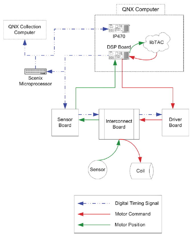
Schematic of the probe electronics showing the data flow and relationships between the main components.

2.3.1. Sensor boards

The primary function of the sensor boards is to convert the analog position sensor output to a scaled, 14-bit digital value. This is accomplished by multiplexing the sensor voltages for 25 motors into the analog to digital (A/D) converter. The addressing is controlled by an EPROM (erasable programmable read-only memory) and involves selecting the sensor voltage for a specific motor just prior to its conversion. The EPROM also controls the timing and synchronization of the A/D conversion by triggering on the FSX signal from the DSP.

Each of the four DSP boards has 4, 16-bit, fixed-point DSPs (TMS320C50PQ, Texas Instruments, Dallas, TX). Each DSP shares dual-ported memory (DPM) space with the PC and uses a 2-megabyte static RAM card (SRAM) for additional program and data storage. The DSP has 8 k words (1 word = 2 bytes) of on-chip RAM available for program execution; 2 k words are shared with the PC via the DPM. An additional 2 k words in the DPM are available to the DSP but hidden from the PC. The SRAM card contains thirty-two 32 k word segments (pages). The motion commands for each of the 25 motors can be stored in pages 1–25. The remaining pages are used for program and coefficient storage. All 16 DSPs are synchronized to a single 40 MHz, clock located on the first DSP board.

2.3.2. Driver boards

The driver boards mirror the functionality of the sensor boards. They receive the motor command from the DSP, convert the digital value to a voltage, amplify it, and apply it to the correct motor coil. Like the sensor boards, the EPM5032 (DIP package, Altera Corporation, San Jose, CA) and the AD7840 D/A (Analog Devices Inc., Norwood, MA) converters use the enable and FSX timing signals from the DSP. The serial data are clocked into the D/A and converted to an analog voltage. The sample-and-hold integrated circuits (ICs) multiplex the voltage to the appropriate amplifier and maintain it until the next motor update. The EPROM controls the addressing and triggers the digital to analog conversion. The LM675 operational amplifier (op amp) (National Semiconductor Corporation, Santa Clara, CA) amplifies the voltage by a factor of five and is directly connected to the motor coil through the interconnect board. As a precautionary measure, the op amp power supply can be switched off with the PS2506 photo-coupler (NEC Electronics Inc, Issaquah, WA). If the “watch-dog” IC, MAX705 (Maxim Integrated Products Inc., Sunnyvale, CA) detects an FSX failure, the EPROM disconnects the amplifier power.

2.3.3. Motor electronics

Each motor has a 20-mm diameter circuit board mounted on the top cap that contains the optosensor. The motor electronics are connected to the interconnect boards with a six conductor wire harness.

2.3.4. Interconnect boards

The sole function of the interconnect boards is to route appropriate signals to and from the various electronic components. The boards are mounted just above and electrically isolated from each plane. The left and right edges have multi-pin edge connectors to attach the sensor board and driver board and one hundred 6-pin headers for each motor.

2.3.5. Positioning the stimulator

The dense array is mounted on a 3-axis stage consisting of three linear positioning tables (LinTech, Monrovia, CA), driven by three servo motors (Baldor, Fort Smith, AR) and a control system (Western Servo Design, Carson City, Nevada). Motion control software and ISA card (Tech80, Plymouth, MN) in a dedicated computer allow accurate and repeatable (within approximately 1 μm) positioning of the probe.

3. Software

The stimulator control and data collection software is written entirely in C++. The software is targeted primarily for use on a real-time QNX operating system, and employs many functions exclusive to this OS. QNX was selected as the OS due to its high level of reliability and real-time performance capabilities. Most of the software can also be run in windows to simulate the behavior of the dense array stimulator for the purpose of testing the protocols offline. The primary C++ stimulator control library is called libTAC, while the protocol- and event-specification library is known as libEVE, both of which are detailed below.

3.1. Dense Array Tactile Control Library (libTAC)

The control library for the dense array converts stimulus specifications provided by the experimenter into voltages that drive each of the 400 motors of the stimulator. Each command determines the position of a pin at time t in the Cartesian z-dimension (perpendicular to the skin surface).

3.1.1. Pin mapping

The 400 pins are mapped in a Cartesian (x, y) plane according to their physical layout in real space. The front, leftmost pin corresponds to mathematical (0, 0) and every other pin is mapped according to its physical location with respect to (0, 0). The individual pins are also numbered from 1 to 400; pin 1 is the back leftmost pin and pin numbering proceeds horizontally across the back, and then wraps around horizontally, so that the front rightmost pin is labeled pin 400.

3.1.2. Protocol architecture

An experimental protocol consists of one or more trials of varying duration, separated by an inter-trial interval, also of varying duration. A trial is composed of five pin movement phases. During the first phase, the 400 pins are held stationary at a pre-specified initial indentation for a given period of time. A ramp phase follows, during which all pins ramp to another indentation amplitude over a period of time, both of which are under the experimenter’s control. During the third phase, any number of stimuli can be presented. For each stimulus, the movement of all or a subset of the pins is defined over a particular duration as described below. During the fourth phase, all 400 pins are again ramped to a given position, making it possible to reverse, if desired, the pre-indentation produced in phase two. The final phase consists of holding the pins at their initial pre-indentation. Typically, at the conclusion of each trial, the 400 pins are returned to their baseline levels, but the pins can be left at any level between trials in order to facilitate fluid trial-to-trial transitions.

3.1.3. Stimulus generation

Each stimulus contains five phases, which are nearly identical to the trial phases detailed above. The important difference is that phase three consists of a function specifying a (typically) more complex pattern of pin movements than a simple ramp. The function contains three components, one or all of which may be used to specify the movement of one or more pins. The three components, described below, are multiplied together to produce the final pin movements. The first component is a uniform multiplier, which scales the movement of each pin specified in the other two components. The second component is a temporal function, allowing pin movements to be specified precisely in time. The third component is a spatio-temporal function, providing the capability to spatially determine pin movement, with or without an additional temporal component. Multiple temporal and spatio-temporal components can be combined to form increasingly more complex pin movements. The position Z of the pin at position (x, y) at time t is thus given by:

$$Z(t,x,y)=a\cdot f_b(t)\cdot f_c(t,x,y)$$ (1)

where a is the scaling factor, f_b(t) a temporal function (e.g., sin(ωt +φ)), and f_c(t, x, y) is a spatio-temporal function (e.g., sin(2π (ft + x/λ) + φ)). The function f_b(t) is defined over time (and not space) and affects all of the pins identically. Typical temporal functions include ramps, sinusoids, and square waves (or rather trapezoidal waves since a true square wave cannot be achieved); f_b(t) can also be set to 1 if the stimulus has no temporal modulation, or if that temporal modulation is pin-specific. In the latter case, it is specified in the spatio-temporal function f_c(t, x, y). The spatio-temporal components of pin movement (f_c(t, x, y)) are generated using one of four modes, or some combination of these, as described in the next section.

(Mode 1) Pin by Pin

The most straightforward mode consists of specifying the position of each pin individually, so that simple spatial patterns, stationary in the (x, y) plane, can be presented on each trial. The Time_on–Time_ramp–Amplitude–Pattern (TTAP) function reads a 20 × 20 bitmap to set the amplitude of each pin for each trial. The pattern is ramped to a pre-specified amplitude beginning at Time_on with respect to the start of the trial and reaches its final position at Time_ramp. The TTAP mode can be used in series to fluidly present various arbitrary spatial patterns (each specified as a separate bitmap). The Time_on–Pin–Amplitude–Waveform (TPAW) function allows even greater control of discrete pin-by-pin movements. Each pin moves through a pre-specified waveform beginning at Time_on. TPAW functions are used in succession to specify the movement of any subset of pins relative to one another in time.

(Mode 2) Unbounded mathematical

Often, one wishes to scan a stimulus with a given displacement profile across the skin. Though the probe does not physically move, this stimulus presentation can be simulated by scanning the pattern across the probe array. In Mode 2, a mathematical function is defined in time over an infinite plane (u, v). The initial position of the (u, v) plane is then specified relative to the origin of the coplanar pin plane (x, y). The (u, v) origin can initially be placed anywhere relative to the (x, y) origin by specifying the vector from the (x, y) origin to the (u, v) origin. The (u, v) origin can be subsequently moved in time relative to the stationary (x, y) plane using any combination of translation and rotation. At each time t, the position of each pin in the (x, y) plane is calculated relative to the (u, v) plane, and the value of the function at that (u, v) location determines the displacement (in the z-dimension) of that pin. LibTAC currently makes use of several different spatial functions defined in the (u, v) plane, including spatio-temporal sinusoids, square waves, annuli, disks, holes, spheres, bars, and corners.

(Mode 3) Bounded Mathematical

Mode 3 builds on Mode 2 by bounding the (u, v) plane and time t, allowing greater control over stimulus onset and offset. “Bounding” the (u, v) plane means that, although a spatial function is specified over the infinite plane, the (u, v) plane is finite. Outside of the boundaries, all values of the spatial function are multiplied by zero, effectively confining the function to a finite region of the plane. Bounding a spatial sinusoid in the u-dimension, for example, would allow a specific number of sinusoidal periods to be created and scanned across the array; these sinusoidal cycles would be trailed by a flat region. The edges of the stimulus along the u or v dimensions can be ramped, providing a means to gradually introduce a stimulus that builds in intensity up to its maximum amplitude. Time is bounded in much the same manner, allowing for abrupt temporal stimulus onset and/or offset or a temporally ramped stimulus, depending on the experimenter’s specifications.

(Mode 4) Hybrid

In the fourth mode, the pin-by-pin specification of Mode 1 is combined with the bounded mathematical specification in Mode 3. The Dot–Amplitude–UV (Dot-AUV) function specifies amplitude much like TTAP and TPAW. But instead of specifically defining which pin the amplitude applies to, Dot-AUV specifies a region of a pre-specified radius in the (u, v) plane within which the displacement is constant. Any pin in (x, y) whose center is located within that region of (u, v) at time t, is commanded to that displacement. Dot-AUV parameters allow the experimenter to design a “field” of cylinders in the (u, v) plane – each defined by its center, radius and amplitude – with any arbitrary spatial configuration. Dot-AUV has been used to generate arbitrary dot patterns varying in density scanned across the array in varying directions at varying velocities. The IMAGE function creates a similar “field” of pixels that form an image in the (u, v) plane. The pixels function exactly like the dots in DOT-AUV, but have a higher density and a fixed radius. This function can be used to scan letters (or similar patterns) across the array.

3.1.4. Filters and conversions

Motors have a tendency to produce undesired vibrations at their resonance frequency. For any type of non-sinusoidal pin movement, resonance distorts the desired waveform. Notch filters can be used to modify the ideal pin-position command signal to compensate for resonance in individual motors.

The notch filter coefficients are calculated using Matlab (Natick, MA) with the optional Control System and System Identification Toolboxes. A model of each motor is created based on an ideal square-pulse command (300 μm amplitude, 100 ms duration) and the resulting motor response. This model is imported into the SISO (Single Input, Single Output) Tool that provides a graphical Bode plot editor. The editor allows the user to place poles and zeros to minimize resonance. The tool can also display the model’s response to a step function, with and without the filter, providing immediate feedback. The resulting six coefficients (for each motor) are written to a file to be used during the final step in the computation of the command signal. The process is automated by iteratively modifying the filter coefficients to minimize the sum of squared differences between desired and actual waveforms. When the optimization algorithm does not yield a satisfactory output signal, the filter parameters are obtained manually (see Fig. 7).

Fig. 7.

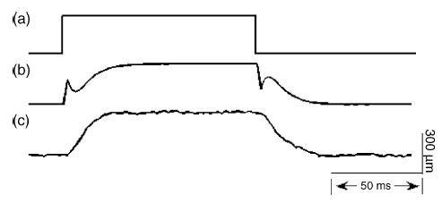
Application of a notch filter to obtain a step indentation: (a) ideal stimulus, consisting of a square pulse; (b) filtered command stimulus (scaled to match the ideal stimulus); (c) motor displacement profile.

When generating sinusoidal stimuli, the notch filter is deactivated in favor of a frequency/amplitude compensation filter. The notch filter tends to distort sinusoidal stimuli, particularly when their frequency is close to the resonance frequency. For sinusoidal stimuli, then, each pin’s amplitude is compensated using a pre-calibrated look-up table that contains a gain factor for each pin at each frequency (within a predetermined set of frequencies). The gain is determined by comparing the actual amplitude, as measured by the (calibrated) optical sensor, with the desired amplitude at a specific frequency (see Fig. 4). A similar calibration process could be effected to compensate for frequency-dependent phase lag.

Once a final pin-position command signal has been determined in microns, the command must be converted into an appropriate voltage value to achieve the desired displacement of the motor. With each motor is associated a polynomial function, obtained during a calibration process (see above), relating command voltage to the resulting amplitude.

3.1.5. DSP interface

When a command is ready to be issued to the stimulator in the form of a voltage, the value is placed in the DPM location of the appropriate DSP controlling the motor. This memory is accessible to both the control computer generating the commands and the DSPs controlling the motors. On each cycle, the signal to be stored in each DSP is laid out motor by motor across all 25 DSPs (each storing the signals for 16 of the 400 motors). To each motor is associated a memory location for the command signal to be sent to that motor and a memory location for its current position. The DSP control rate is set at 1 kHz. During each cycle, the DSPs deliver each command to the corresponding motor at the correct time, read the current position of each motor, then store it in the dual-ported memory so that the control computer can access position data.

3.1.6. Command cycles and synchronization

The command cycle is matched to the DSP control rate (1 kHz); in other words, each motor is updated with a new command every millisecond. The synchronization between the completion of a command cycle and the creation of the next set of pin positions is managed using the master clock of the DSPs and a microprocessor. Each command cycle of the 16 DSPs (one of which is governed by a master clock) begins with a distinct level change on a digital line. An 8-bit Scenix microprocessor (Ubicom, Inc., Sunnyvale, CA) interrupts each time the level change occurs, allowing the device to monitor the cycle timing of the DSPs. The microprocessor sends a digital interrupt signal to the dense array control computer at the beginning of each cycle. The interrupt signal triggers a chain of events. The control computer writes out the latest pin position commands of all 400 pins, reads the current position of the pins, then calculates the next position of each pin, all prior to the completion of the DSP cycle.

In addition to governing the probe command cycle, the Scenix microprocessor sends out a digital interrupt signal at pre-specified intervals, which are multiples of the DSP cycle. This synchronization signal can be sent to any machine (e.g., a spike collection system) that needs to be tightly coupled with the stimulus.

3.1.7. Pin positions

During the command cycle, the control computer reads the current position of each pin according to the output of the nonlinear optical displacement sensors. These values are linearized using polynomial fit functions generated for each sensor during the pin calibration process. These polynomial functions are used to convert output from the optical sensors into displacements (Fig. 5). The pin position data are also stored to a file for later analysis. The cycle-by-cycle displacement can also be fed back into the motor servo control system, when running the system in closed loop mode.

3.1.8. Open-loop/closed-loop servo control

The dense array stimulator motors can be run in either a closed-loop servo mode or an open-loop, zero-feedback mode. Closed-loop servo control can produce more faithful pin movements for certain non-sinusoidal stimuli, but results in high-frequency jitter. This jitter is caused by noisy sensor data and by the limited speed of the hardware (specifically the DSPs), which prevents servo control at rates greater than 1 kHz. At this servo cycle rate, pin position updates are too slow to implement filters to reduce high-frequency noise.

Open loop control produces superior sinusoidal stimuli and accurate non-sinusoidal stimuli with the use of the notch filter discussed above (see Figs. 4 and 7). The stimulator is currently run exclusively in open loop mode in order to maximize pin position accuracy while minimizing high frequency noise. The skin is sufficiently compliant relative to the motor spring constants to have little effect on pin movements (see above).

3.2. Event specification library (libEVE)

The dense array protocols are specified by the experimenter in a State Block File, which is converted into an Event File. The Event File (or one of its derivatives) is used to specify control on the input side of the dense array, and to store the stimulus and the corresponding neural responses on the output side.

3.2.1. Event file format

The event file format (EVE) is a binary file format consisting of chronologically ordered events. Each event is composed of a 64-bit double-precision floating-point time value, a 64-bit integer code, and a variable bit-length value. The time specifies the time at which the event occurred; the code details the type of event; the value may be a single number, a string, a vector of numbers or strings, or a matrix of numbers or strings and characterizes the critical parameter for that event (see below).

3.2.2. State block file format

The state block file (SBF) format is derived directly from the EVE file format. An SBF is a text-based file specifying stimulus events without any specified time, only a code and a value. The state of the stimulator is defined in the SBF file in well-defined blocks, each of which characterizes all of the experimental events/parameters relevant to a period of experimental time. There are six primary periods for which blocks must be defined: the beginning of the protocol, the beginning of a trial, the onset and offset of a stimulus, the end of a trial, and the end of the protocol.

3.2.3. Protocol specification overview

Any information required to fully specify a given protocol, trial, or stimulus is provided as a state in the SBF. The amplitude of a sinusoid, for example, would be specified using a unique code and paired with a value indicating the desired amplitude. This value would be set in a state block at the beginning of the stimulus, and the system will use the value when generating pin positions. The state of the probe can be set at any time using event commands, including specifications of the temporal and spatio-temporal functions to be invoked, the amplitude and duration of the stimulus, etc. Combining a wide assortment of event commands allows for precise control of pin movement over the course of a protocol.

4. Applications

As mentioned above, one of the main advantages of the stimulator is that it allows the user to generate arbitrary spatio-temporal stimuli “on the fly.” The only limitations are the amplitude (approximately 2 mm peak to peak) and size of the stimuli, currently limited to 1 cm². In a series of studies, we have used the array to generate a variety of stimuli using different modes of stimulus generation. We present some of these modes here.

The simplest and most straightforward tactile stimulus is the statically indented spatial pattern. In this mode, the stimulus is first specified as a 20 × 20 pixilated pattern (typically consisting of values ranging from −1 to 1), each element of which represents the relative amplitude of each probe in the array. For the simplest applications, the duration of the on- and off-ramps is specified, as well as the peak amplitude of the stimulus (the factor by which the pixilated image needs to be multiplied to yield the desired indentation amplitude of each pin in the array). The advantage of dissociating relative amplitude from maximum amplitude is that the maximum amplitude present in the pattern is made explicit and can thus easily be stored during data collection. In the simple ramp-and-hold mode, spatial patterns such as gratings, sinusoids, spheres, and letters can be generated, as long as the temporal profile of the stimulus simply consists of an initial on-ramp, a sustained phase, and an off-ramp. These types of stimuli were used in a study to generate a continuum mechanical model of mechanoreceptive afferent responses to arbitrary spatial patterns (Sripati et al., 2006a). Another application of this stimulus-generation mode is receptive field mapping. Individual probes are indented into the skin in random order, and the evoked responses are plotted in a 20 × 20 bitmap, each pixel representing the response elicited by the corresponding probe. The resulting map reveals the size and structure of the neuron’s receptive field (Fig. 8). A more sophisticated illustration of receptive field mapping is the computation of spatio-temporal receptive fields from both peripheral and cortical responses to spatio-temporal white noise (Sripati et al., 2006b) (see Fig. 9).

Fig. 8.

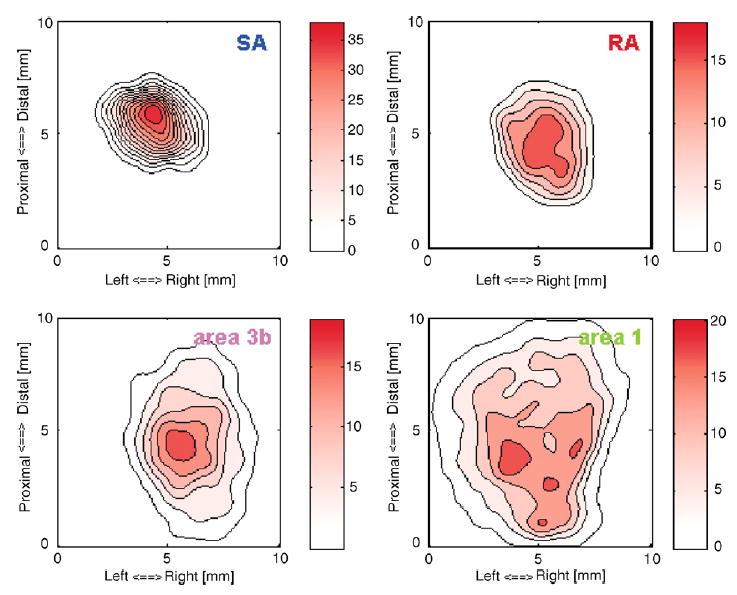
Receptive field map obtained from a typical SA1 fiber (top left), RA fiber (top right), neuron in area 3b (bottom left), and neuron in area 1 (bottom right). Responses are initially represented as a 20 × 20 array of pixels, each or which shows the response elicited in the neuron when a probe at that location is indented into the skin. In the above plots, contours have been superimposed upon this RF map, after it has been passed through a two-dimensional Gaussian (σ = 0.5 mm). The color bars indicate the response in spikes per second. Mean response maps such as these highlight differences in the spatial layout of the receptive fields of different cells along the somatosensory pathway.

Fig. 9.

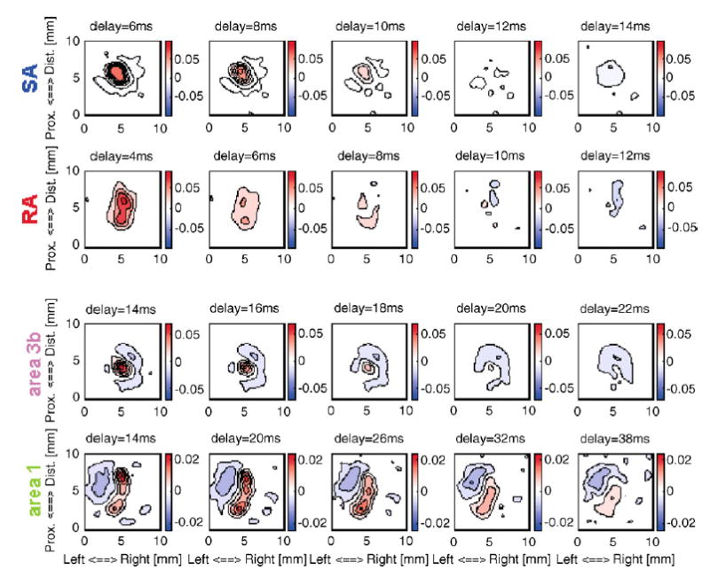
Spatio-temporal receptive fields for an SA1 fiber, and RA fiber, a neuron in area 3b and a neuron in area 1. Using the stimulator, the dynamic properties of the receptive fields of somatosensory neurons can be characterized. Each figure shows the mean effect of a pin indentation at each location in the receptive field on the neural response as a function of the delay following stimulus onset. The color bars indicate the regression weights applied to that region at that time interval. For instance, the top right figure shows the effect of pin indentations across the array on the neural response 14 ms after these indentations as a function of their location within the array. The initially excitatory effect of pin indentations observed at a 6-ms delay (top left figure) has changed to an inhibitory effect due to relative refractoriness in this SA fiber.

The ramp-and-hold mode can be modified in two ways basic ways. The pattern can be multiplied by an arbitrary mathematical function or the pattern can be translated in any direction and at any speed (limited only by the refresh rate of the display). The multiplicative function consists in taking a 3-D spatial stimulus profile and multiplying it by an arbitrary function. For example, if a square wave pattern (consisting of 0 s and 1 s) is multiplied by a temporal sinusoid, the ridges of the wave (specified as 1 s in the 20 × 20 bitmap) will oscillate at a frequency and amplitude specified by the parameters of the sinusoids. Such vibrating gratings were used in a pair of studies investigating the relationship between vibratory frequency and the spatial modulation in the neural response. The neural response of first-order afferents was compared with psychophysically measured spatial acuity for the same stimuli (Bensmaia et al., 2006a,b).

In some cases, both the spatial and temporal properties of the stimulus can be specified simply as a mathematical function. For instance, a spatio-temporal sinusoid (such as those presented in Bensmaia et al., 2006c) can be generated using the appropriate mathematical function (Fig. 10). Again, the maximum amplitude is typically 1 and then scaled up or down using a multiplicative factor, so that stimulus amplitude is always explicit in the state block file.

Fig. 10.

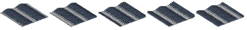
Sequence of snapshots depicting a spatio-temporal sinusoid (with a spatial period of 5 mm) drifting across the array (similar to those presented in Bensmaia et al., 2006c). Because the density of the pins exceeds the innervation density in the glabrous skin of humans, the stimulus is perceived as a smooth, undulating surface.

Another common stimulus-generation mode consists of defining a spatial pattern and “moving” the spatial pattern across the array. In this mode, the stimulus is once again defined as a 20 × 20 pattern, with its starting position, its direction of motion, and its speed specified. The position of the stimulus is first defined in a hypothetical coordinate system and then projected onto the array so the starting position of the stimulus can be outside the array. When the trial begins, the stimulus is translated across the array at the specified velocity starting at the selected starting location. As described, the translation is computed at a higher resolution than that of the probe, resulting in smooth motion across the array.

In the previous paragraphs, we described modes with which stimuli can be generated rapidly and precisely without the need to machine patterns. However, the major advantage of the dense array is that it allows the experimenter to (1) present a large number of completely different spatio-temporal patterns in a short period of time and (2) to generate spatio-temporal patterns adaptively during the course of an experiment.

It is often desirable to determine the responses of a neuron to both static stimuli as well as to dynamic stimuli. In the study of visual processing, cells in the primary visual cortex can be categorized in terms of their orientation selectivity, and a subset of these orientation-selective cells also exhibit direction selectivity. To fully characterize the responses of these cells, both static and dynamic stimuli are typically used. With the dense array, a wide variety of both moving and static stimuli can be presented to a given neuron. In macaque monkeys, a peripheral afferent or cortical neuron can be held for approximately 1–2 h. With the dense array, stimulus durations typically range from 50 to 200 ms. Thus, over 72,000 stimuli of short duration (50 ms) can be presented during the course of a 2-h-long recording session. From the neural responses to such an extensive stimulus set, the properties of a neuron can be characterized to a large stimulus space. In a set of ongoing experiments, we record the responses of both peripheral afferents and neurons in the primary somatosensory cortex to a wide range of stimuli, including scanned or indented edges, corners, spheres, gratings, random dot patterns, etc. From these responses, we characterize both the peripheral and central representations of tactile stimuli, and the sensory transformation that these representations undergo from periphery to cortex.

An important advantage of generating stimuli “on the fly” is that it allows us to generate these stimuli adaptively. One of the major problems in sensory neuroscience is that it is often impossible to present stimuli that span the entire stimulus space, if the stimuli vary along multiple dimensions (see e.g., Brincat and Connor, 2004). For example, spatio-temporal sinusoids can vary in their wavelength, temporal frequency, amplitude, and orientation. For even such a relatively simple stimulus, if 10 levels were sampled along each dimension, the stimulus set would consist of 10⁴ stimuli. The difficulty in machining these stimuli and presenting them during the session is obvious. Therefore, it is often desirable to tailor a stimulus to a neuron so that only stimuli that are within that neuron’s response space are presented. Because the dense array allows us to precisely map a given cell’s receptive field, we can reduce the number of stimulus presentations and present only stimuli that fall within the receptive field. Furthermore, we can measure the directional selectivity of that cell (using random dot patterns that drift in different directions, for example), and then present patterns that vary in their spatial configuration but are moving in the cell’s preferred direction. If one had to combine all of the shapes with all of the directions, the stimulus set would be too large to be presented within a single recording session. The ability to adapt the stimulus set “on-line” allows us to sample more densely the stimulus space relevant to a given neuron.

The ability to generate stimuli adaptively is important in human psychophysical measurements as well. For example, in adaptive procedures used to determine absolute levels of performance, the next stimulus to be presented depends upon the subject’s previous responses. Such adaptive psychophysical procedures concentrate observations near the subject’s threshold and are generally more efficient than the method of constant stimuli and other classical psychophysical approaches (Fechner, 1860).

References

- Bensmaia SJ, Craig JC, Johnson KO. Temporal factors in tactile spatial acuity: evidence for RA interference in fine spatial processing. J Neurophysiol. 2006a;95:1783–91. doi: 10.1152/jn.00878.2005. [DOI] [PMC free article] [PubMed] [Google Scholar]
- Bensmaia SJ, Craig JC, Yoshioka T, Johnson KO. SA1 and RA afferent responses to static and vibrating gratings. J Neurophysiol. 2006b;95:1771–82. doi: 10.1152/jn.00877.2005. [DOI] [PMC free article] [PubMed] [Google Scholar]
- Bensmaia SJ, Killebrew JH, Craig JC. The influence of visual motion on tactile motion perception. J Neurophysiol. 2006c;96:1625–37. doi: 10.1152/jn.00192.2006. [DOI] [PMC free article] [PubMed] [Google Scholar]
- Blake DT, Hsiao SS, Johnson KO. Neural coding mechanisms in tactile pattern recognition: the relative contributions of slowly and rapidly adapting mechanoreceptors to perceived roughness. J Neurosci. 1997;17:7480–9. doi: 10.1523/JNEUROSCI.17-19-07480.1997. [DOI] [PMC free article] [PubMed] [Google Scholar]
- Bliss JC, Katcher MH, Rogers CH, Shepard RP. Optical-to-tactile image conversion for the blind. IEEE Trans Man-Machine Sys MMS-11. 1970:58–65. [Google Scholar]
- Brincat SL, Connor CE. Underlying principles of visual shape selectivity in posterior inferotemporal cortex. Nat Neurosci. 2004;7:880–6. doi: 10.1038/nn1278. [DOI] [PubMed] [Google Scholar]
- Connor CE, Hsiao SS, Phillips JR, Johnson KO. Tactile roughness: neural codes that account for psychophysical magnitude estimates. J Neurosci. 1990;10:3823–36. doi: 10.1523/JNEUROSCI.10-12-03823.1990. [DOI] [PMC free article] [PubMed] [Google Scholar]
- Connor CE, Johnson KO. Neural coding of tactile texture: comparisons of spatial and temporal mechanisms for roughness perception. J Neurosci. 1992;12:3414–26. doi: 10.1523/JNEUROSCI.12-09-03414.1992. [DOI] [PMC free article] [PubMed] [Google Scholar]
- DiCarlo JJ, Johnson KO. Velocity invariance of receptive field structure in somatosensory cortical area 3b of the alert monkey. J Neurosci. 1999;19:401–19. doi: 10.1523/JNEUROSCI.19-01-00401.1999. [DOI] [PMC free article] [PubMed] [Google Scholar]
- DiCarlo JJ, Johnson KO. Spatial and temporal structure of receptive fields in primate somatosensory area 3b: effects of stimulus scanning direction and orientation. J Neurosci. 2000;20:495–510. doi: 10.1523/JNEUROSCI.20-01-00495.2000. [DOI] [PMC free article] [PubMed] [Google Scholar]
- DiCarlo JJ, Johnson KO. Receptive field structure in cortical area 3b of the alert monkey. Behav Brain Res. 2002;135:167–78. doi: 10.1016/s0166-4328(02)00162-6. [DOI] [PubMed] [Google Scholar]
- DiCarlo JJ, Johnson KO, Hsiao SS. Structure of receptive fields in area 3b of primary somatosensory cortex in the alert monkey. J Neurosci. 1998;18:2626–45. doi: 10.1523/JNEUROSCI.18-07-02626.1998. [DOI] [PMC free article] [PubMed] [Google Scholar]
- Fechner GT. In: Elements of Psychophysics. Adler HE, translator. New York: Holt, Rinehart and Winston; 1966. 1860. [Google Scholar]
- Gardner EP, Palmer CI. Simulation of motion on the skin. I. Receptive fields and temporal frequency coding by cutaneous mechanoreceptors of Optacon pulses delivered to the hand. J Neurophysiol. 1989;62:1410–36. doi: 10.1152/jn.1989.62.6.1410. [DOI] [PubMed] [Google Scholar]
- Johnson KO. The roles and functions of cutaneous mechanoreceptors. Curr Opin Neurobiol. 2001;11:455–61. doi: 10.1016/s0959-4388(00)00234-8. [DOI] [PubMed] [Google Scholar]
- Johnson KO, Hsiao SS. Neural mechanisms of tactual form and texture perception. Annu Rev Neurosci. 1992;15:227–50. doi: 10.1146/annurev.ne.15.030192.001303. [DOI] [PubMed] [Google Scholar]
- Johnson KO, Phillips JR. Tactile spatial resolution. I. Two-point discrimination, gap detection, grating resolution, and letter recognition. J Neurophysiol. 1981;46:1177–91. doi: 10.1152/jn.1981.46.6.1177. [DOI] [PubMed] [Google Scholar]
- Johnson KO, Phillips JR. A rotating drum stimulator for scanning embossed patterns and textures across the skin. J Neurosci Methods. 1988;22:221–31. doi: 10.1016/0165-0270(88)90043-x. [DOI] [PubMed] [Google Scholar]
- Johnson KO, Yoshioka T, Vega-Bermudez F. Tactile functions of mechanoreceptive afferents innervating the hand. J Clin Neurophysiol. 2000;17:539–58. doi: 10.1097/00004691-200011000-00002. [DOI] [PubMed] [Google Scholar]
- Mountcastle VB, LaMotte RH, Carli G. Detection thresholds for stimuli in humans and monkeys: comparison with threshold events in mechanoreceptive afferent nerve fibers innervating the monkey hand. J Neurophysiol. 1972;35:122–36. doi: 10.1152/jn.1972.35.1.122. [DOI] [PubMed] [Google Scholar]
- Nefs HT, Kappers AM, Koenderink JJ. Amplitude and spatial-period discrimination in sinusoidal gratings by dynamic touch. Perception. 2001;30:1263–74. doi: 10.1068/p3217. [DOI] [PubMed] [Google Scholar]
- Pawluk DT, Howe RD. Dynamic lumped element response of the human finger-pad. J Biomech Eng. 1999;121:178–83. doi: 10.1115/1.2835100. [DOI] [PubMed] [Google Scholar]
- Pawluk DTV, van Buskirk CP, Killebrew JH, Hsiao SS, Johnson KO. Control and pattern specification for a high density tactile display. In: Furness RJ, editor. Proceedings of the ASME dynamic systems and control division, ASME international mechanical engineering congress and exposition. DSC-vol 64. 1998. pp. 97–102. [Google Scholar]
- Phillips JR, Johansson RS, Johnson KO. Representation of Braille characters in human nerve fibers. Exp Brain Res. 1990;81:589–92. doi: 10.1007/BF02423508. [DOI] [PubMed] [Google Scholar]
- Phillips JR, Johansson RS, Johnson KO. Responses of human mechanoreceptive afferents to embossed dot arrays scanned across fingerpad skin. J Neurosci. 1992;12:827–39. doi: 10.1523/JNEUROSCI.12-03-00827.1992. [DOI] [PMC free article] [PubMed] [Google Scholar]
- Phillips JR, Johnson KO. Tactile spatial resolution. II. Neural representation of bars, edges, and gratings in monkey primary afferents. J Neurophysiol. 1981;46:1192–203. doi: 10.1152/jn.1981.46.6.1192. [DOI] [PubMed] [Google Scholar]
- Phillips JR, Johnson KO, Hsiao SS. Spatial pattern representation and transformation in monkey somatosensory cortex. Proc Natl Acad Sci USA. 1988;85:1317–21. doi: 10.1073/pnas.85.4.1317. [DOI] [PMC free article] [PubMed] [Google Scholar]
- Sripati AP, Bensmaia SJ, Johnson KO. A continuum mechanical model of mechanoreceptive afferent responses to indented spatial patterns. J Neurophysiol. 2006a;95:3852–64. doi: 10.1152/jn.01240.2005. [DOI] [PMC free article] [PubMed] [Google Scholar]
- Sripati AP, Yoshioka T, Denchev P, Hsiao SS, Johnson KO. Spatiotemporal receptive fields of peripheral afferents and cortical area 3b and 1 neurons in the primate somatosensory system. J Neurosci. 2006b;26:2101–14. doi: 10.1523/JNEUROSCI.3720-05.2006. [DOI] [PMC free article] [PubMed] [Google Scholar]
- Summers IR, Chanter CM. A broadband tactile array on the fingertip. J Acoust Soc Am. 2002;112:2118–26. doi: 10.1121/1.1510140. [DOI] [PubMed] [Google Scholar]
- Yoshioka T, Gibb B, Dorsch AK, Hsiao SS, Johnson KO. Neural coding mechanisms underlying perceived roughness of finely textured surfaces. J Neurosci. 2001;21:6905–16. doi: 10.1523/JNEUROSCI.21-17-06905.2001. [DOI] [PMC free article] [PubMed] [Google Scholar]