Magnetic Resonance Spectroscopic Imaging Reconstruction With Deformable Shape-Intensity Models

Abstract

A new method, based on a deformable shape-intensity model (DSM), was developed to improve the signal-to-noise ratio (SNR) of multidimensional magnetic resonance spectroscopic imaging (MRSI) data sets without affecting spectral lineshapes and linewidths. Improvements with DSM, compared to digital filters using conventional signal apodization, were demonstrated on both simulated and experimental in vivo ¹H MRS images from 22 cognitively normal (CN) elderly subjects and 25 patients with Alzheimer's disease (AD). Simulated MRSI data showed that DSM achieved superior noise suppression compared to a matched apodization filter. Experimental MRSI data showed that SNR could be increased 2.1-fold with DSM without distorting spectral resolution, thus maintaining all spectral features of the raw, unfiltered data. In conclusion, DSM should be used to achieve high SNR in reconstructing MRSI data.

In vivo magnetic resonance spectroscopic imaging (MRSI) suffers generally from poor signal-to-noise ratio (SNR), because of a combination of a weak MR signal and low metabolite concentrations. Low SNR limits the technique's ability to detect metabolite abnormalities in subjects. Therefore, an increase of SNR is a key factor in the success of many MRSI applications. Signal averaging is one way to improve SNR. However, this approach is often not practical because of long acquisition times. In addition, signal averaging can become inefficient with higher B₀ fields, because physiological noise, which scales with the magnetic field strength, increasingly contributes to variations of the signal (1). Another way to improve SNR is by noise suppression using digital filters. This is conventionally achieved by multiplying MRSI data in the time domain with exponential functions (apodization filters) that are designed to attenuate high-frequency noise in MR spectra (2,3). A carefully designed apodization filter that “matches” line-width of the metabolite signal can reduce noise without degrading spectral resolution (2). However, matched filtering is difficult to accomplish in MRSI because linewidths, as well as lineshapes, often vary substantially over large regions in the brain (4,5).

Methods that model spectral signal characteristics, such as intensity and frequency, may help resolve the difficulties that arise with the use of spectral apodization filters. Deformable shape-intensity models (DSMs) are being used in digital image analysis (6-8) to maintain essential characteristics of image shape and intensity while accommodating fluctuations. These models have not been applied before to MRSI; however, the frequency and intensity variations of MRSI may be interpreted in a similar manner as for the shape and intensity fluctuations of images, which suggests that DSM might be useful in analyzing MRSI data. In this study, we applied DSM to process MRSI data to improve SNR. The specific goals were to 1) develop DSM for separating in complex-valued MRSI data coherent modulations of both intensity and phase from random fluctuations, thus suppressing noise; and 2) compare DSM with spectral apodization filters in improving SNR of MRSI, and the effect on a subsequent automated spectral analysis procedure. Studies were carried out using both simulated and experimental data. Furthermore, to demonstrate that DSM is applicable to a wide range of MRSI data, including biological variability of metabolite distributions, we analyzed MRSI from a large group of cognitively normal (CN) elderly subjects and patients with Alzheimer's disease (AD) with DSM.

THEORY

MRSI data, which are usually obtained by Fourier transformation of a spatially encoded MR signal and represented as a multidimensional data array, can also conveniently be expressed as a (N× L) complex-valued matrix X with columns representing spectra at each spatial location k = 1 … N, hence s(r_k, ω), and rows representing spectral images at each frequency j = 1 … L, hence s(r,ω_j). Here, r = (x₁, y₁, z₁, … x_k, y_k, z_k, … x_N, y_N, z_N)^T is a vector with N components for each spatial location and r_k = (0, 0, 0, … x_k, y_k, z_k, … 0, 0, 0)^T. Similarly, ω = (ω₁ … ω_j … ω_L)^T is a vector with L components, each representing a particular spectral frequency. Note that the term “spectral image” refers to a set of spatial data points (2D or 3D) at a particular spectral frequency ω_j, as opposed to the term “spectroscopic image,” which represents a metabolite map that is usually derived by integrating over a frequency range. The matrix representation of MRSI data is thus

$$\mathbf{X}=\left[\begin{array}{ccc}\hfill s(r_1,{\omega }_1)\hfill & \hfill \cdot \hfill & \hfill s(r_N,{\omega }_1)\hfill \\ \hfill \cdot \hfill & \hfill s(r_k,{\omega }_j)\hfill & \hfill \cdot \hfill \\ \hfill s(r_1,{\omega }_L)\hfill & \hfill \cdot \hfill & \hfill s(r_N,{\omega }_L)\hfill \end{array}\right].$$ [1]

The hypothesis behind this concept was that regional variations of metabolite peaks in MRSI could be described as fluctuations of intensities and frequencies around a mean spectrum of all spatial locations $\stackrel{‒}{\mathbf{x}}=(1∕N){\sum }_{k=1}^{N}s({\mathbf{r}}_k,\omega )$. Further, we hypothesized that the principal modes of the fluctuations could be represented by a weighted sum of eigen-spectral images ${\mathbf{p}}_j=s(\mathbf{r},{\omega }_j^{\mathrm{E}})$, where ${\omega }^{\mathrm{E}}={\left({\omega }_1^{\mathrm{E}}\dots {\omega }_L^{\mathrm{E}}\right)}^{\mathrm{T}}$ are eigen-frequencies, representing both coherent fluctuations (metabolite peaks) and random noise. Thus, the jth spectral image can be parameterized by a linear model of the form

$${\mathbf{x}}_j=s(\mathbf{r},{\omega }_j)=\stackrel{‒}{\mathbf{x}}+{\mathbf{Pb}}_j.$$ [2]

Here, the columns of matrix P of order (N × L) are the eigen-spectral images p₁ … p_L, and b_j = (b₁ … b_L)^T holds the weights of each p_j in composing the spectral image x_j. P can be obtained by principal components analysis (PCA) (8). This involves decomposition of an L × L covariance matrix of X into eigenvectors, summation of fluctuations around the mean spectrum, and finally back-projection of the spectral images onto the eigen-space (see Appendix). Vectors b_j can be obtained by multiplying Eq. [2] with P^T, the matrix transpose of P, and since P^TP = I for eigen-spectral images, one immediately obtains

$${\mathbf{b}}_j={\mathbf{P}}^{\mathrm{T}}({\mathbf{x}}_j-\stackrel{‒}{\mathbf{x}}).$$ [3]

A new spectral image y_j that has in principle the same characteristic as x_j, but exhibits less noise, can then be constructed with DSM by linear combinations of the mean spectrum and weighted sums of selected eigen-spectral images according to:

$${\mathbf{y}}_j=\stackrel{‒}{\mathbf{x}}+\widehat{\mathbf{P}}{\mathbf{b}}_j+\epsilon .$$ [4]

Here, the matrix P̂ of order (N × M) with M < L is a subset of P, and ε is a vector of mean differences (errors) between the experimental x_j and modeled y_j spectral images. The variance of ε is given by $\sigma ={\sum }_{j=M+1}^L{\lambda }_j$ (9), where λ_j are eigenvalues of the remaining L-M-1 eigen-spectral images. If all L eigen-spectral images were utilized to reconstruct y_j, ε would be zero (9). To reduce noise, only a subset M < L of eigen-spectral images, represented by P̂, should be used for reconstruction, which inevitably results in a finite value for ε and σ. Subsets P̂ can be selected in decreasing order of importance, i.e., in order of the ranked eigenvalues λ_j > λ_j+1, with the assumption that large eigenvalues correspond to metabolite resonances and small eigenvalues correspond primarily to noise. The selection criterion for the order (N × M) of P̂ depends primarily on the accumulative magnitudes of λ_j. The optimal size of P̂ can be obtained by a simple exhaustive search for the minimum of an error function, as described by Davies et al. (10). Furthermore, because eigenvalue series usually decrease quickly, it is often sufficient for all practical purposes to select an even smaller subset than the optimal size for reconstruction of noise-reduced data. Equation [4] also shows that the basis of the SNR improvement is the fact DSM operates on all data combined, rather than on single spectra, as do conventional apodization filters. Therefore, one would expect that noise reduction with DSM is more efficient for 2D and 3D MRSI, where many spectra are available, than for single-voxel data.

METHODS

Computer Simulations

Noise Reduction

Noise reduction with DSM was tested first on simulated brain MRSI data. Brain spectroscopic images of N-acetylaspartate (NAA), creatine (Cr), choline (Cho), and myo-inositol (MI) were simulated by transforming a synthetic brain map into k-space and time domains, according to:

$$\begin{array}{cc}\hfill s(\mathbf{k},t)=\mathrm{FFT}& {}^{-1}\{\sum _{\mathit{tiss}=1}^4\sum _{m=1}^4\rho {(\mathbf{r},\mathit{tiss})}_m\hfill \\ \hfill & \cdot e^{-i[2\pi {\nu }_m+\Delta \omega \left(\mathbf{r}\right)]t}\cdot e^{-[t∕T_{\mathrm{Lor}}+{(t∕T_{\text{Gauss}})}^2]}+\mathit{noise}\}.\hfill \end{array}$$ [5]

The brain was based on MRI brain model 152 of the International Consortium for Brain Mapping (ICBM) (11). Here, s(k, t) is the MRSI data in the k-t domain after inverse Fourier transformation (FFT⁻¹) of the simulated regional metabolite distribution ρ(r, tiss) of metabolite m for each tissue type, tiss, taken over all spatial locations, r. ν_m is a metabolite resonance (for simplicity, only a single resonance frequency was assumed for each metabolite), Δω(r) represents local magnetic field variations, T_Lor and T_Gauss are Lorentzian and Gaussian signal decays, and i = √−1. Summations are for different tissue types and the four metabolites. The simulation parameters are summarized in Table 1. s(k, t) in Eq. [5] and s(r, ω_j) in Eq. [2] are related by Fourier transformation, and s(r, ω_j) is a cross section of MRSI. To compare noise reduction with DSM and apodization filtering, MRSI data were simulated for eight different noise levels. Noise was generated using a random-number generator from IDL Libraries (Research System; Kodak Company, CO). Gaussian apodization filters of 1.3, 3.0, and 5.0 Hz width (full width at half height) were used to simulate typical experimental conditions. After the data were filtered, image reconstruction of s(k, t) was performed using an automated spectral analysis and metabolite image formation package (12). Three categories of noisy MRSI data sets were generated for comparisons: 1) DSM-filtered data, 2) apodization-filtered data, and 3) unfiltered raw data. The “gold standard” was an MRSI set without noise.

Table 1.

Spectral Parameters for Simulation of MRSI Data

Substance	Brain tissue	Frequencya	Concentrationb	Linewidtha
Water	CSF	0.0	100.0	8.0
Lipid	Scalp + lipid	−204.8	100.0	80.0
MI	White matter	−75.6	12.0	5.0
	Grey matter	−75.6	8.0	5.0
Cho	White matter	−97.3	16.0	5.0
	Grey matter	−97.3	24.0	5.0
Cr	White matter	−107.5	28.0	5.0
	Grey matter	−107.5	21.0	5.0
NAA	White matter	−172.8	40.0	5.0
	Grey matter	−172.8	30.0	5.0

^aResonance frequency and linewidth in Hertz.

^bIn arbitrary units.

DSM and Spatial Resolution

To determine whether DSM filtering could have a detrimental effect on the detection of small regions with altered signal intensity, a small circular lesion of total signal loss surrounded by an area of homogeneous metabolite intensities was simulated for a range of sizes from 4 to 22 mm in diameter. SNR was set to 15:1. To assess whether the effective spatial resolution was affected by the different filter methods, the metabolite contrast in the lesion center was evaluated as a function of lesion diameter. Results from DSM and a matched apodization filter were compared to the resolution in the gold-standard MRSI.

Human Brain Data

Comparisons between DSM and the apodization filters were performed for NAA and MI on experimental in vivo MRSI data from 22 elderly CN subjects (nine men and 13 women, mean age = 72.1 ± 8.5 years) and 25 patients with a clinical diagnosis of AD (eight men and 17 women, mean age = 73.0 ± 6.21 years), who were clinically evaluated at the Aging Centers of the University of California (UC)–San Francisco and UC–Davis as part of another MRI and MRSI study in this laboratory. The study was approved by the committee of human research at the UC–San Francisco, and all subjects gave written informed consent before they participated in the study. MRSI was performed on a 1.5 T MR scanner (Vision; Siemens Medical Systems, Iselin, NJ) using a multislice sequence with a short spin-echo time of 25 ms and lipid signal nulling by slice-selective inversion recovery, as described previously (13). Three 15-mm-thick axial oblique MRSI slices with a nominal in-plane resolution of (0.75 mm)² were acquired. To reduce further lipid contamination, a fully automated procedure to detect extracranial lipid regions was used together with an iterative method for k-space extrapolation (14). Subsequently, brain tissue masks were also automatically generated, and spectra from regions outside the brain were ignored. Large MRSI datasets (64 × 64 × 256 points) were processed by DSM in <1 min on a Pentium 4 PC computer at 1.8 GHz. The spectral analysis and metabolite image formation package (12) was applied, including calculations of Cramer-Rao minimum variance bounds (CRBs) (15) to estimate the accuracy of the spectral fitting. The root mean square (RMS) noise of the experimental data was measured after baseline correction in the spectral range between −1.8 and −3.6 ppm, approximately 2.4 ppm downfield from the NAA resonance (16,17).

In a first attempt to evaluate the effectiveness of DSM for reducing noise in in vivo MRSI data, we compared the number of spectra that had acceptable quality after the DSM or apodization filters were applied. The following criteria for acceptable quality of spectra were used (18): First, metabolic linewidth, as estimated with automated fitting, had to be between 1.9 and 11.1 Hz. Second, the difference between MI and Cr fitted resonance frequencies had to be between 0.43 and 0.63 ppm. Third, the difference between Cr and NAA resonance frequencies had to be between 0.97 and 1.05 ppm. In further attempts to quantitatively evaluate DSM, we employed statistical tests as described in the following section.

Statistics

Differences between DSM and apodization filters for SNR were determined with simulated MRSI data by subtracting a noiseless gold-standard MRSI dataset from the filtered MRSI sets. The subtraction provided a measure of the extent to which the different filter methods recovered the MRSI gold standard. Differences between DSM- and apodization-filtered data were tested using paired t-tests. To determine whether DSM or a matched apodization filter had an effect on spatial resolution, two-tailed t-tests were used. To determine whether differences between filtering methods mattered for in vivo MRSI data, given the biological variability between subjects, an analysis of variance (ANOVA) was used with subject and filter methods as independent variables and metabolite intensities as dependent variables. Post-hoc Scheffe tests were used for pairwise comparisons of filters, and the threshold of significance was increased to α = 0.001 to avoid finding effects by chance. Furthermore, to evaluate the performance of DSM over a wide range of metabolite images, including MRSI data from normal subjects and patients, an ANOVA with factors for group (CN or AD), filters (raw, apodization, or DSM), and an interaction between the two was used to determine metabolite variations. Finally, to quantify the similarity between unfiltered and filtered MRSI data (either by DSM or by apodization filters), intra-class correlation coefficients (ICCs) were computed (19).

RESULTS

Simulations

Simulated NAA (top row) and MI (bottom row) images with typical SNRs for NAA of 9:1 and for MI of 3:1 are shown in Fig. 1, with different filtering methods applied. DSM improved SNR better than apodization with a matched Gaussian filter, as seen, for example, by increased delineation of ventricular boundaries in the DSM-filtered MI image. For comparison, the gold-standard metabolite images are also shown in Fig. 1 on the far left.

FIG. 1.

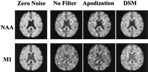
Simulated NAA (top) and MI (bottom) intensity maps.

Figure 2 demonstrates the effects of different filters in recovering NAA intensity from simulated MRSI data with high and low SNR. Also plotted in Fig. 2 for comparison are the results when MRSI data were not filtered (black bars). This shows that the error in recovering NAA intensity was less with DSM (P < 0.0001) than with apodization filters of different widths (no filter, 1.3, 3.0, and 5.0 Hz Gaussians) at both high and low SNR. Figure 2 further shows that for apodization filters, the errors depend in a complicated manner on SNR and filter width.

FIG. 2.

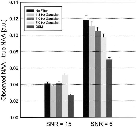
Errors in recovering NAA intensity in simulated MRSI data with low and high SNRs after application of different filters.

The effects of DSM and apodization filters on spatial blurring, as simulated by a small region of reduced NAA intensity, are shown in Fig. 3. Also shown for comparison is the gold-standard NAA intensity. Intensity profiles show the well-known Gibbs ringing effect, which is exacerbated by a rapid signal drop at the edge of the simulated lesion. DSM resulted in a small intensity increase by about 1.24% ± 0.9%, compared to the gold standard, while matched Gaussian apodization resulted in an intensity decrease by about 1.84% ± 0.8%. However, the difference between DSM and Gaussian apodization was not significant. These differences further decreased with increasing SNR, as expected.

FIG. 3.

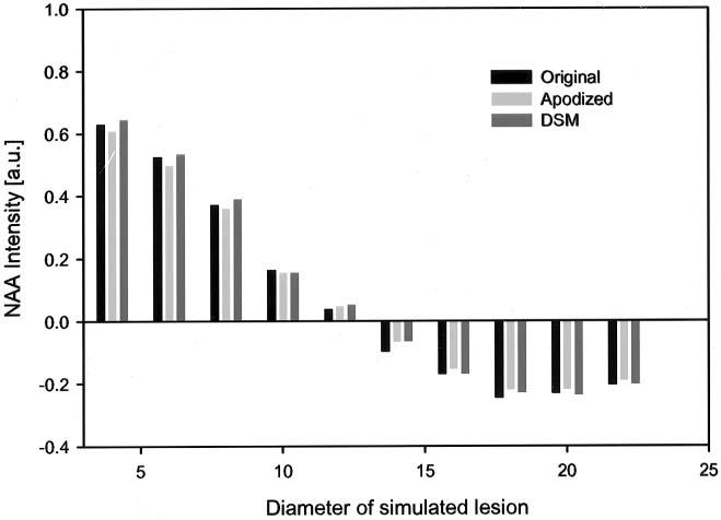
Effect of DSM and a 1.3-Hz apodization filter in detecting a small lesion in a homogenous region (simulated MRSI data). The NAA intensity at the center of the small signal void is plotted as a function of the diameter of that region.

Experimental Data

A representative ¹H MRSI spectrum of parietal lobe gray matter from a 74-year-old CN subject is shown in Fig. 4, processed using either DSM or apodization filters of different widths (1.3, 3.0, and 5.0 Hz Gaussians). The unfiltered spectrum is also shown. This demonstrates an exquisite improvement in SNR with DSM. Furthermore, spectral resolution is not sacrificed with DSM, as seen by the separation of Cho and Cr in the spectrum at the bottom (arrow). In contrast to DSM, apodization filtering progressively degraded the spectral resolution, with increasing suppression of noise.

FIG. 4.

Representative ¹H MR spectrum from parietal cortical gray matter from a 74-year-old CN subject. The spectrum is shown unfiltered (top), after apodization filtering using different widths (middle), and after DSM filtering (bottom). Heavy apodization filtering degraded spectral resolution, in contrast to DSM (see arrow).

Table 2 lists results from automated fitting of 44695 experimental ¹H MR spectra from 22 control subjects with no filter application, and after filtering with either DSM or a 1.3-Hz Gaussian apodization filter. Listed are the average RMS noise, the metabolite linewidth, and the percentage of satisfactorily fitted spectra, as defined by the criteria listed in Methods. Compared to unfiltered data, noise suppression was 53% with DSM and 38% with the 1.3-Hz Gaussian apodization filter. The estimated line-width of metabolite resonances increased on average by 0.3 Hz with DSM, and by 0.9 Hz with the apodization filter, from an estimated linewidth of 5 Hz in unfiltered MRSI data.

Table 2.

Effect of Filters on Quality of MR Spectra^*

	RMS noisea	Linewidthb	Poor fitc
No filter	7.2 ± 1.7	5.02 ± 2.19	5.57%
Apodization	4.5 ± 1.5	5.90 ± 2.20	5.82%
DSM	3.4 ± 1.5	5.27 ± 2.17	3.94%

^*Results from 44,695 MR spectra from 22 control subjects using no spectral filters, a Gaussian apodization filter of 1.3 Hz width, or DSM.

^aRMS: root mean square.

^bLinewidth in Hz.

^cPercentage of spectra in MRSI that did not meet following criteria: 1) linewidth between 1.9 and 11.1 Hz; 2) fitted resonance difference between MI and Cr between 0.43 and 0.63 ppm; and 3) fitted resonance difference between NAA and Cr between 0.97 and 1.05 ppm.

Representative metabolite images of NAA (top row) and MI (bottom row) are shown in Fig. 5, processed without filter (left column), with a Gaussian apodization filter (middle column), and with DSM (right column). Marked improvements in discerning anatomical structures can be seen in the MI image after processing with DSM.

FIG. 5.

Representative metabolite images of NAA and MI from a 77-year-old CN subject. Unfiltered, apodized, and DSM-filtered images are displayed using the same intensity level.

Figure 6 shows results from CRB computations on a representative MRSI dataset from a 72-year-old AD patient. The graph shows changes of CRB values as a function of apodization filter width for fits of NAA area, frequency, T_Lor, and T_Gauss. As expected, CRB values decrease as filter width increases. Also shown in the graph are the corresponding CRB values from noise reduction with DSM, which demonstrate smaller CRB values than obtained with apodization filters. Also depicted in Fig. 6 are maps of CRB values for fitted NAA areas (the corresponding NAA image is shown on the far right). This again demonstrates the superiority of DSM compared to apodization filtering in achieving highest quality of fits. High CRB values in frontal brain regions primarily resulted from poor spectral resolution. In addition, CRB maps related to the apodization filters show high values in some parietal brain regions (arrows), where the spectra were usually of good quality. This indicates that CRB values can markedly increase locally with heavy apodization filtering, although globally CRB values decreased with apodization, as shown in the graph.

FIG. 6.

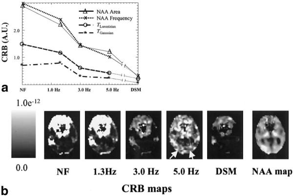
a: CRB values from fits of in vivo MR spectra as a function of spectral filtering. Results are averaged from 406 ¹H MR spectra of white matter from a 72-year-old patient with AD. CRB values are calculated for NAA area, NAA frequency, and a combination of Lorentzian (T_Lor,) and Gaussian (T_Gauss) signal decays. b: Regional distribution of CRB values for the NAA area from the same MRSI data as above. Arrows indicate increased CRB values from heavy (5.0 Hz) apodization filtering, which is not observed with DSM or mild apodization filtering.

To further evaluate the difference between DSM and apodization filters in experimental MRSI data, histograms of MI intensity from 14218 MR spectra of white matter from the 22 CN subjects were compared. Figure 7a shows the MI histograms of raw MRSI (solid curve) and MRSI processed with DSM (dashed curve) or a Gaussian apodization filter (dotted curve). This shows a strong similarity between raw and DSM-filtered data, while MI intensities are markedly shifted toward lower values after the Gaussian apodization filter was applied, indicating an intensity bias by the filter. ANOVA showed an overall significant effect from the different filters (F_2,42651 = 378, P < 0.001 ). Post-hoc Scheffe tests revealed that this effect was primarily caused by Gaussian apodization filtering, which led to differences between filtered and unfiltered MI data (P < 0.001), while no significant difference was introduced with DSM. Similar results were obtained for histograms of NAA intensity, as depicted in Fig. 7b. As for MI, changes in NAA intensities were associated with filter method (F_2,42651 = 190, P < 0.001). Post-hoc Scheffe tests again showed that this effect was primarily caused by apodization filtering, which led to differences between filtered and unfiltered NAA data (P < 0.001), while no significant difference was introduced with DSM. The similarity between DSM and unfiltered data was also demonstrated by ICCs (19) between unfiltered and filtered MRSI data. Here, an ICC of 1 indicates perfect similarity and 0.5 means no similarity. A comparison between unfiltered and DSM-filtered MRSI data yielded ICCs of 0.98 and 0.95 for MI and NAA, respectively. In contrast, unfiltered and apodization-filtered MRSI data produced ICCs of 0.54 and 0.90 for MI and NAA, respectively (see Table 3a), while DSM and apodization-filtered MRSI data yielded ICCs of 0.54 and 0.82 for MI and NAA, respectively.

FIG. 7.

Histograms of MI and NAA intensities from ¹H MR spectra of white matter in 22 CN controls and 25 AD patients. The histograms illustrate similarities between unfiltered MRSI data and filtered MRSI data using either a 1.3-Hz Gaussian apodization filter or DSM.

Table 3.

Comparisons Between Unfiltered, Apodized, and DSM Filtered MRSI Data of MI and NAA of White Matter

	MIa	ICCMIb	NAAa	ICCNAAb
a. Normal subjectsc
No filter	13.3 ± 3.0	–	24.2 ± 4.8	–
Apodization	12.5 ± 2.7e	0.54	23.3 ± 4.3e	0.90
DSM	13.2 ± 2.8	0.98	24.2 ± 4.5	0.95
b. AD patientsd
No filter	13.3 ± 4.6	–	23.3 ± 5.8	–
Apodization	12.5 ± 4.0e	0.79	22.2 ± 5.2e	0.73
DSM	13.3 ± 4.4	0.95	23.2 ± 5.6	0.98

^aMean metabolite intensity ± standard deviation.

^bICC, intraclass correlation coefficients between filtered (apodization or DSM) and unfiltered data. An ICC of 1 reflects a perfect correlation, an ICC of 0.5 indicated no correlation.

^cMRSI data from 22 cognitive normal controls with a total of 14,218 spectra of white matter.

^dMRSI data from 25 patients with Alzheimer's disease with a total 11,777 spectra of white matter.

^eP < 0.001 for filtered versus unfiltered MRSI.

Finally, we tested whether DSM would yield similar results in another large MRSI dataset from 25 patients with AD, who usually present larger metabolite variability than normal subjects. The results, shown in Fig. 7c and d and listed in Table 3b, were similar to those obtained in control subjects. To determine whether DSM affected MRSI data from CN subjects and AD patients equally, we modeled differences between intensity histograms as a function of both filters and group (CN and AD) using ANOVA. This revealed no group by filter interaction for either MI (F_3,51986 = 0.2, P > 0.05) or NAA (F_3,51986 = 0.1, P > 0.05), indicating that DSM had an equal effect on both patient and control data.

DISCUSSION

We have described the use of DSM to reconstruct MRSI data, and demonstrated that the model was superior to conventional apodization filters in improving SNR without degrading spectral resolution.

DSM has previously been used for image analysis in face recognition and detection of brain structures, among other applications (6-8, 20-22). These previous applications of DSM involved only magnitude images to model shape and intensity variations, whereas in the current study we extended DSM to the complex domain for MRSI, which includes variations of both magnitude and phase of the signal. Applying DSM to magnitude MRSI data would have resulted in loss of phase information (23), and the use of both the real and imaginary components of the spectra theoretically provides a √2 better SNR (24,25).

The first advantage of DSM compared to apodization filters was a substantial reduction of noise. The extent of the SNR improvement depends in part on the ability of the model to retrieve coherent information from the data, and is proportional to the number of spectra included in the calculation of the model. Hence, a large number of spectra must be available to efficiently reduce noise with DSM. Because MRSI datasets consist of a large number of spectra, which are utilized collectively by DSM, the model can be built with minimum noise content, while preserving the major linear correlation in data. A potential pitfall of this approach is that the inclusion of poor-quality spectra could lead to the generation of suboptimal eigen-spectal images. Therefore, spectra of poor quality should be removed before application of DSM for maximal performance. Poor spectral quality often results from extracranial lipid and residual water signal contaminations in regions close to the scalp, eyes, and sinuses. We demonstrated an automated approach for eliminating poor-quality spectra to ensure high performance of DSM by reducing total noise variance (26). Taken together, the results indicate that DSM improved the SNR for both computer-simulated and experimental MRSI data compared to conventional apodization methods, and yielded metabolite images of better contrast between brain tissues. Results from in vivo MRSI data showed a 2.1-fold increase in SNR with DSM, compared to a 1.6-fold increase with using apodization filters. It is expected that the advantage of DSM compared to apodization filters increases further if more MR spectra are available, i.e., with volumetric MRSI.

The second advantage of DSM compared to apodization filters was that spectral resolution was not sacrificed as noise suppression improved. Although increased apodization filter weighting will result in an SNR similar to that obtained with DSM, this can only be achieved with apodization filters at the expense of spectral degradation. This is not surprising, because apodization filters achieve noise reduction based on the principle of band limitation, which suppresses any signal outside a frequency range, regardless of whether it is related to resonances or noise. In contrast, DSM is designed to separate coherent from non-coherent resonances without band limitation, thus suppressing selectively noise. Results from CRB calculations, which are an accepted means of estimating fitting quality (27,28), also demonstrated the superiority of DSM over apodization filters. The importance of maintaining spectral resolution is further emphasized by findings of other studies that showed increased CRB values for overlapping resonance lines (29). In short, an important advantage of the DSM over an apodization filter is better spectral resolution for equivalent SNR.

In this study, we used DSM to model variations of both spectral lineshapes and signal intensities to reconstruct the original MRSI for the purpose of suppressing noise. As the results from both simulations and in vivo MRSI data from 47 subjects showed, DSM achieved noise reductions with minimal effects on linewidth and other spectral features, including baseline, as demonstrated by a high similarity between NAA and MI histograms from DSM-filtered and unfiltered data sets (see histograms in Fig. 7). In contrast, MRSI data processed with apodization filters deviated substantially from the original data by bias toward lower metabolite intensities. This problem with apodization filters has potential implications for the quantification of metabolites.

The present implementation of DSM was developed in the frequency domain and therefore was compromised by problems related to Fourier transformation, such as artifacts due to data truncation in time and k-space domains. In principle, DSM could also be applied directly to ¹H MRSI data in the time domain to avoid complications from Fourier transformations, similarly to singular value decomposition methods in combination with Cadzow enhancement procedures (30-33). A time-domain approach of DSM should benefit reconstruction of MRSI data, especially in the presence of temporal irregular signal modulations (i.e., due to flow or movement) (32). A number of other MRS applications might also benefit from DSM, especially in vivo ³¹P and ¹³C MRSI, which usually suffer from poor SNR. The DSM algorithm can be also extended to accommodate multidimensional and multiecho spectroscopy (34). In addition to MRSI, the concept of complex-domain DSM should be applicable to the reconstruction of signal evolution in dynamic MRI data, including perfusion and functional MRI.

APPENDIX

Here we present the computation of eigen-spectral images p_j. Let x_j = s(r, ω_j) be a spectral image of N voxels at a particular spectral frequency ω_j, with j = 1 … L. Further, let ${\stackrel{‒}{\mathbf{x}}}_j=(1∕N){\sum }_{k=1}^{N}s({\mathbf{r}}_k,{\omega }_j)$ be the average peak intensity from all k voxels at ω_j. Then a difference matrix D with size (N × L) can be defined according to

$$\mathbf{D}=\left(({\mathbf{x}}_1-{\stackrel{‒}{x}}_1)\dots ({\mathbf{x}}_j-{\stackrel{‒}{x}}_j)\dots ({\mathbf{x}}_L-{\stackrel{‒}{x}}_L)\right).$$ [A1]

The N × N covariance matrix C of D, can be obtained according to

$$\mathbf{C}=\frac{1}{N}{\mathbf{DD}}^{\mathrm{T}}.$$ [A2]

Because only L eigen-spectral images are required, let T be a smaller covariance matrix of size (L × L)

$$\mathbf{T}=\frac{1}{N}{\mathbf{D}}^{\mathrm{T}}\mathbf{D}.$$ [A3]

Let e_j (j = 1 … L) be the eigenvector of T with corresponding eigenvalues λ_j,:

$${\mathbf{Te}}_j={\lambda }_j{\mathbf{e}}_j.$$ [A4]

Substituting T from Eq. [A3] into Eq. [A4] yields

$$\frac{1}{N}{\mathbf{D}}^{\mathrm{T}}{\mathbf{De}}_j={\lambda }_i{\mathbf{e}}_j.$$ [A5]

Premultiplying by D results in:

$$\frac{1}{N}{\mathbf{DD}}^{\mathrm{T}}{\mathbf{De}}_j={\lambda }_i{\mathbf{De}}_j$$ [A6]

and therefore

$$\mathbf{C}\left({\mathbf{De}}_j\right)={\lambda }_j\left({\mathbf{De}}_j\right).$$ [A7]

Thus, if e_j is an eigenvector of T, then De_j is an eigenvector of C and has the same eigenvalue. Using each of L eigenvectors De_j, and each of L eigenvalues λ_j, an eigen-spectral image can be constructed by projecting the sum of fluctuations from the mean spectrum, D, onto the eigen-space of e:

$${\mathbf{p}}_j=\frac{1}{\sqrt{N{\lambda }_j}}{\mathbf{De}}_j.$$ [A8]

If the eigenvalues are ranked according to their magnitude, the first complex eigen-spectral image, associated with the largest eigenvalue, accounts for most of the MRSI information, and subsequent eigen-spectral images contain progressively less information (35) until they reach the level of noise.

REFERENCES

- 1.Kruger G, Kastrup A, Glover GH. Neuroimaging at 1.5 T and 3.0 T: comparison of oxygenation-sensitive magnetic resonance imaging. Magn Reson Med. 2001;45:595–604. doi: 10.1002/mrm.1081. [DOI] [PubMed] [Google Scholar]
- 2.Sanders JKM, Hunter KH. Spectroscopy. Oxford University Press; Oxford, UK: 1987. p. 302. [Google Scholar]
- 3.Bartha R, Drost DJ, Williamson PC. Factors affecting the quantification of short echo in-vivo 1H MR spectra: prior knowledge, peak elimination, and filtering. NMR Biomed. 1999;12:205–216. doi: 10.1002/(sici)1099-1492(199906)12:4<205::aid-nbm558>3.0.co;2-1. [DOI] [PubMed] [Google Scholar]
- 4.Gonen O, Grossman RI. The accuracy of whole brain N-acetylaspartate quantification. Magn Reson Imaging. 2000;18:1255–1258. doi: 10.1016/s0730-725x(00)00221-6. [DOI] [PubMed] [Google Scholar]
- 5.Li BS, Regal J, Gonen O. SNR versus resolution in 3D 1H MRS of the human brain at high magnetic fields. Magn Reson Med. 2001;46:1049–1053. doi: 10.1002/mrm.1297. [DOI] [PubMed] [Google Scholar]
- 6.Cootes TF, Edwards GJ, Taylor CJ. Active appearance models. IEEE PAMI. 2001;23:681–685. [Google Scholar]
- 7.Nastar C, Moghaddam B, Pentland A. Generalized image matching: statistical learning of physically-based defomations. Comput Vis Image Underst. 1997;65:179–191. [Google Scholar]
- 8.Turk M, Pentland A. Eigenfaces for recognition. J Cogn Neurosci. 1991;3:71–86. doi: 10.1162/jocn.1991.3.1.71. [DOI] [PubMed] [Google Scholar]
- 9.Hyvarinen A, Oja E. Independent component analysis: algorithms and applications. Neural Netw. 2000;13:411–430. doi: 10.1016/s0893-6080(00)00026-5. [DOI] [PubMed] [Google Scholar]
- 10.Davies RH, Twining CJ, Cootes TF, Waterton JC, Taylor CJ. A minimum description length approach to statistical shape modeling. IEEE Trans Med Imaging. 2002;21:525–537. doi: 10.1109/TMI.2002.1009388. [DOI] [PubMed] [Google Scholar]
- 11.Kwan RK, Evans AC, Pike GB. MRI simulation-based evaluation of image-processing and classification methods. IEEE Trans Med Imaging. 1999;18:1085–1097. doi: 10.1109/42.816072. [DOI] [PubMed] [Google Scholar]
- 12.Soher BJ, Young K, Govindaraju V, Maudsley AA. Automated spectral analysis III: application to in vivo proton MR spectroscopy and spectroscopic imaging. Magn Reson Med. 1998;40:822–831. doi: 10.1002/mrm.1910400607. [DOI] [PubMed] [Google Scholar]
- 13.Wiedermann D, Schuff N, Matson GB, Soher BJ, Du AT, Maudsley AA, Weiner MW. Short echo time multislice proton magnetic resonance spectroscopic imaging in human brain: metabolite distributions and reliability. Magn Reson Imaging. 2001;19:1073–1080. doi: 10.1016/s0730-725x(01)00441-6. [DOI] [PubMed] [Google Scholar]
- 14.Haupt CI, Schuff N, Weiner MW, Maudsley AA. Removal of lipid artifacts in 1H spectroscopic imaging by data extrapolation. Magn Reson Med. 1996;35:678–687. doi: 10.1002/mrm.1910350509. [DOI] [PMC free article] [PubMed] [Google Scholar]
- 15.Ober RJ, Lin Z, Ye H, Ward ES. Achievable accuracy of parameter estimation for multidimensional NMR experiments. J Magn Reson. 2002;157:1–16. doi: 10.1006/jmre.2002.2560. [DOI] [PubMed] [Google Scholar]
- 16.Young K, Soher BJ, Maudsley AA. Automated spectral analysis II: application of wavelet shrinkage for characterization of non-parameterized signals. Magn Reson Med. 1998;40:816–821. doi: 10.1002/mrm.1910400606. [DOI] [PubMed] [Google Scholar]
- 17.Soher BJ, Young K, Maudsley AA. Representation of strong baseline contributions in 1H MR spectra. Magn Reson Med. 2001;45:966–972. doi: 10.1002/mrm.1129. [DOI] [PubMed] [Google Scholar]
- 18.Ebel A, Soher BJ, Maudsley AA. Assessment of 3D proton MR echo-planar spectroscopic imaging using automated spectral analysis. Magn Reson Med. 2001;46:1072–1078. doi: 10.1002/mrm.1301. [DOI] [PubMed] [Google Scholar]
- 19.Shrout PE, Fleiss JL. Intraclass correlations: uses in assessing rater reliability. Psychol Bull. 1979;2:420–428. doi: 10.1037//0033-2909.86.2.420. [DOI] [PubMed] [Google Scholar]
- 20.Covell M. Control-point location using principal component analysis; Proceedings of the 2nd International Conference on Automatic Face and Gesture Recognition; Killington. 1996. pp. 122–127. [Google Scholar]
- 21.Moghaddam B, Pentland A. Probabilistic visual learning for object recognition. IEEE Trans Patt Anal Machine Intell. 1997;19:696–710. [Google Scholar]
- 22.Cootes TF, Taylor CJ, Cooper D, Graham J. Active shape models—their training and application. Comput Vis Image Understand. 1995;61:38–59. [Google Scholar]
- 23.Witjes H, Melssen WJ, in't Zandt HJ, van der Graaf M, Heerschap A, Buydens LM. Automatic correction for phase shifts, frequency shifts, and lineshape distortions across a series of single resonance lines in large spectral data sets. J Magn Reson. 2000;144:35–44. doi: 10.1006/jmre.2000.2021. [DOI] [PubMed] [Google Scholar]
- 24.Stoyanova R, Brown TR. NMR spectral quantitation by principal component analysis. NMR Biomed. 2001;14:271–277. doi: 10.1002/nbm.700. [DOI] [PubMed] [Google Scholar]
- 25.Elliott MA, Walter GA, Swift A, Vandenborne K, Schotland JC, Leigh JS. Spectral quantitation by principal component analysis using complex singular value decomposition. Magn Reson Med. 1999;41:450–455. doi: 10.1002/(sici)1522-2594(199903)41:3<450::aid-mrm4>3.0.co;2-9. [DOI] [PubMed] [Google Scholar]
- 26.Brown TR, Stoyanova R. NMR spectral quantitation by principal-component analysis. II. Determination of frequency and phase shifts. J Magn Reson B. 1996;112:32–43. doi: 10.1006/jmrb.1996.0106. [DOI] [PubMed] [Google Scholar]
- 27.Cavassila S, Deval S, Huegen C, van Ormondt D, Graveron-Demilly D. Cramer-Rao bound expressions for parametric estimation of overlapping peaks: influence of prior knowledge. J Magn Reson. 2000;143:311–320. doi: 10.1006/jmre.1999.2002. [DOI] [PubMed] [Google Scholar]
- 28.Young K, Khetselius D, Soher BJ, Maudsley AA. Confidence images for MR spectroscopic imaging. Magn Reson Med. 2000;44:537–545. doi: 10.1002/1522-2594(200010)44:4<537::aid-mrm7>3.0.co;2-8. [DOI] [PubMed] [Google Scholar]
- 29.Slotboom J, Boesch C, Kreis R. Versatile frequency domain fitting using time domain models and prior knowledge. Magn Reson Med. 1998;39:899–911. doi: 10.1002/mrm.1910390607. [DOI] [PubMed] [Google Scholar]
- 30.Cadzow JA. Signal enhancement—a composite property mapping algorithm. IEEE Trans Acoust Speech Signal Process. 1988;36:49–62. [Google Scholar]
- 31.Lin YY, Hwang LP. NMR signal enhancement based on matrix property mappings. J Magn Reson Ser A. 1993;103:109–114. [Google Scholar]
- 32.Vanhamme L, Sundin T, Hecke PV, Huffel SV. MR spectroscopy quantitation: a review of time-domain methods. NMR Biomed. 2001;14:233–246. doi: 10.1002/nbm.695. [DOI] [PubMed] [Google Scholar]
- 33.Coron A, Vanhamme L, Antoine JP, Van Hecke P, Van Huffel S. The filtering approach to solvent peak suppression in MRS: a critical review. J Magn Reson. 2001;152:26–40. doi: 10.1006/jmre.2001.2385. [DOI] [PubMed] [Google Scholar]
- 34.Michaeli S, Garwood M, Zhu XH, DelaBarre L, Andersen P, Adriany G, Merkle H, Ugurbil K, Chen W. Proton T2 relaxation study of water, N-acetylaspartate, and creatine in human brain using Hahn and Carr-Purcell spin echoes at 4T and 7T. Magn Reson Med. 2002;47:629–633. doi: 10.1002/mrm.10135. [DOI] [PubMed] [Google Scholar]
- 35.Watanabe S. Karhunen-Loeve expansion and factor analysis; Transactions of the 4th Prague Conference on Information Theory, Statistical Decision Function, Random Processes; Prague. 1965. pp. 635–657. [Google Scholar]