

Abstract
Recent high-throughput genotyping technologies, such as the Affymetrix 500k array and the Illumina HumanHap 550 beadchip, have driven down the costs of association studies and have enabled the measurement of single-nucleotide polymorphism (SNP) allele frequency differences between case and control populations on a genomewide scale. A key aspect in the efficiency of association studies is the notion of “indirect association,” where only a subset of SNPs are collected to serve as proxies for the uncollected SNPs, taking advantage of the correlation structure between SNPs. Recently, a new class of methods for indirect association, multimarker methods, has been proposed. Although the multimarker methods are a considerable advancement, current methods do not fully take advantage of the correlation structure between SNPs and their multimarker proxies. In this article, we propose a novel multimarker indirect-association method, WHAP, that is based on a weighted sum of the haplotype frequency differences. In contrast to traditional indirect-association methods, we show analytically that there is a considerable gain in power achieved by our method compared with both single-marker and multimarker tests, as well as traditional haplotype-based tests. Our results are supported by empirical evaluation across the HapMap reference panel data sets, and a software implementation for the Affymetrix 500k and Illumina HumanHap 550 chips is available for download.
Large-scale case-control association studies are a potentially powerful tool for discovering the genetic basis of human disease.1–3 Recent high-throughput genotyping technologies, such as the Affymetrix 500k array and the Illumina HumanHap 550 beadchip, have driven down the costs of association studies and have allowed us to measure allele frequency differences between case and control populations on a genomewide scale.4,5 A key aspect in the efficiency of association studies is the notion of “indirect association.” By leveraging the linkage disequilibrium (LD) structure of the genome, frequency differences between case and control populations do not need to be measured in all SNPs but only in a subset, or a set of tag SNPs that serve as proxies for the remaining uncollected SNPs (we also refer to the uncollected SNPs as “hidden SNPs”).6 A chromosome carrying a particular allele of a tag SNP has a high probability of carrying a particular allele of a proximal hidden SNP. Thus, an allele frequency difference in a hidden SNP will manifest itself as an allele frequency difference in a tag SNP. This correlation is often measured between two SNPs by the correlation coefficient r2. The r2 measure is widely used in the design and analysis of association studies, because the relation between the power of detecting an association at the hidden SNP and only observing the tag SNP has been well understood for some time (e.g., see the work of Pritchard and Preworzski7 and Sham et al.8).
Tag SNPs are chosen by examining the LD structure of a reference panel such as the HapMap,9 which is a data set that contains a complete set of genotypes from 270 individuals, with >3.9 million SNPs across the genome. Choosing a set of tag SNPs is a challenging problem, since the LD structure is quite complex and varies through the genome. To date, many tag SNP selection methods have been proposed.10,11 These methods employ different statistical criteria, the most common being procurement of a set of tag SNPs for which every hidden SNP is “covered” by a tag SNP, such that the correlation coefficient r2 between the two SNPs in the reference set is higher than a certain threshold (e.g., see the work of Carlson et al.11). These methods vary greatly in the optimization methods used to obtain the tag SNPs.
Recently, a new class of methods—multimarker methods—has been proposed.10,12–14 These methods take advantage of the fact that some pairs (or groups) of SNPs serve as better proxies for the hidden SNPs than does any single SNP. Since multimarker proxies have more than two possible alleles, the frequencies of a specific sequence of alleles in these SNPs (i.e., a haplotype) are compared between the cases and the controls. Thus, a specific haplotype, instead of a single SNP, is used as a proxy for a hidden SNP. It has been shown empirically that these methods can reduce the number of tags required to achieve equivalent power.10 In addition, it has been empirically shown that even if the set of tag SNPs is fixed—such as in the case where a commercial high-throughput genotype product is used—one can choose a set of multimarkers for each hidden SNP and considerably increase the r2 (and therefore the power) between that proxy haplotype and the hidden SNP.15
Although multimarker methods are a considerable advancement, current methods do not fully take advantage of the correlation structure between SNPs and their multimarker proxies. For example, consider the scenario given in figure 1. In this example, we assume that the first two SNPs are collected as tag SNPs for the association study and will be used as proxies for the three remaining SNPs. The third SNP is in perfect disequilibrium with the first SNP (r2=1), and, thus, the first SNP serves as a perfect proxy for the third SNP. Since the fourth SNP is not in perfect disequilibrium with either of the first two SNPs, the haplotype AA at the first two SNPs can serve as a perfect proxy for the fourth SNP. The most interesting case is the fifth SNP, for which no haplotype serves as a perfect proxy. The best haplotype proxy for this SNP is the haplotype AA, for which r2=0.619. However, by restricting ourselves to the haplotype AA, we ignore the additional information given by the other haplotypes. For example, the allele A in the fifth SNP occurs occasionally with haplotype AG, but never with haplotypes GA or GG.
Figure 1. .

A sample haplotype distribution for five SNPs, where the first two SNPs are collected as tag SNPs, and the remaining three SNPs are uncollected. Freq. = frequency.
To take advantage of this additional information, we propose a new statistic, the ρ test, and a new method, WHAP, that is based on a weighted sum of all the haplotype frequency differences. We show both empirically and analytically that there is a considerable gain in power achieved by this statistic, as opposed to a χ2 statistic on a single SNP or group of haplotypes. We show that the ρ test is χ2 distributed with 1 df, regardless of the weight assignments. We then develop a notion equivalent to r2, defined by the haplotype weights r2h and with values ranging from 0 to 1. Analogously to Pritchard and Preworzski,7 we show that, if a multimarker set has a correlation of r2h with a causal SNP, then using the ρ test with n/r2h individuals for this set is equivalent to directly testing the causal SNP for association with n individuals. We show analytically that the r2h for a set of tag SNPs is always at least as large as the best r2 for any single haplotype or single SNP. Empirically, we observe that, in many cases, r2h is, in fact, quite larger than r2, which leads to a significant increase in power. For instance, in the above example, the correlation coefficient between the weighted average of the haplotypes and the fifth SNP is 0.85, whereas it is only 0.619 for the best single haplotype. Finally, we show that the ρ test is always more powerful than the standard χ2 test over a set of haplotypes. Our proposed method uses a statistic similar to the one proposed in the works of Nicolae16 and Stram.17
Previous approaches for tag SNPs, such as single-marker and multimarker approaches involving one haplotype, fall into our framework, since these can be seen as specific assignments of weights to the haplotypes (i.e., letting the weight of the haplotype be 1 and the weight of all the other haplotypes be 0). We present a method to find the optimal set of weights that maximizes the power of the ρ statistic, and we show both analytically and empirically that our method always performs at a power equal or greater to standard multimarker methods. Furthermore, we show that, asymptotically, one can gain power only by using a larger number of SNPs as a proxy to the hidden SNP. In practice, since sample size is limited, “overfitting” effects may reduce power, and we therefore empirically show that, for haplotypes of moderate length, there is an increase in power. To the best of our knowledge, this is the first rigorous analytical proof that demonstrates that haplotype and multimarker indirect association is asymptotically more powerful than indirect association based on single SNPs.
Our methods and power analysis relies on accurate haplotype frequency estimates. Since the accuracy of haplotype frequency estimation depends on different factors, such as the number of SNPs used, their physical locations, and the LD structure, we evaluated our analytical results via simulation. We first demonstrate that r2h is always >r2 for both SNPs and multimarker tags over the marker sets of the Affymetrix 500k and Illumina HumanHap 550 chips. In particular, moving from multimarker tags to our WHAPs results in up to a 21.1% increase in the number of captured common SNPs (minor-allele frequency [MAF] ⩾0.05 and r2 or r2h ⩾0.8). Second, we simulate case-control panels under various disease models and show that this increase in utility corresponds, as expected, to an increase in the power of our method compared with the use of single SNPs and multimarker tags.
We calculated the optimal weights for every HapMap phase II SNP, using the Affymetrix 500k and Illumina HumanHap 550 SNP sets. These data are available on request, and the software for performing association tests that use WHAPs can be downloaded from the WHAP Web site.
Material and Methods
The ρ test is a statistic that is applied to a set of WHAP tag SNPs that are a proxy for the hidden SNP. It can be used in place of the standard χ2 statistic applied to the tag SNPs. Informally, the ρ test computes a weighted sum of all the tag SNP haplotype frequency differences between the case and control samples. A more formal description of the ρ test is given below.
In traditional multimarker methods, for a given hidden SNP, a set of SNPs are chosen as tag SNPs, and a specific haplotype of the tag SNPs is used as the proxy. In contrast, in the ρ test framework, once the tag SNPs are chosen, a weight for each of the haplotypes is determined. The specific values of the weights are estimated from the reference panel (e.g., the HapMap data set) and are recorded for each hidden SNP.
The ρ test is χ2 distributed with 1 df, and its power depends on the correlation coefficient r2h between the statistic and the hidden SNP (see below). We show that r2h is analogous to r2 in standard association methods, in the sense that it provides a direct linear relation to power.
We consider the setting in which an association study is performed on N cases and N controls. We assume that the causal SNP s is not genotyped but that a set of SNPs, § ={s1,…,sm}, in LD with s are genotyped. For simplicity of presentation, we assume that each of the SNPs is biallelic, with allele values 0 and 1. To distinguish the allelic notation of s from that of the other SNPs, we assume that the alleles of s are C and c. Let h1,…,hk∈{0,1}m be the set of haplotypes over the set of SNPs §. We suggest a statistical test, the ρ test, which is based on a convex combination of the haplotype frequencies. This combination depends on the joint distribution of the alleles c and C of s and the haplotypes in the HapMap data.
Formally, let  be a set of haplotype weights. Let
  and
and  be the observed frequencies of haplotype h in the case and control populations, respectively, and let
  . We define the ρ statistic as
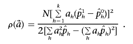 |
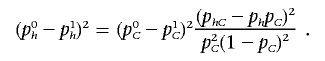
Under the null hypothesis,  is distributed as χ2 with 1 df—that is, the square of a standard normal distribution. With p0h and p1h denoting the true frequency of haplotype h in the case and control populations, respectively, under the alternate hypothesis,
  is distributed as the square of a normal distribution with mean
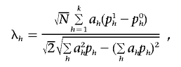 |
where the variance is ∼1, with the assumption that p1h≈p0h and that ph=(p0h+p1h)/2. Thus, the power of the  statistic depends on the frequencies p0h and p1h and on the weight vector
  .
.
To evaluate the statistical power of the  statistic, we are interested in comparing its power with the power of detecting association directly with the causal SNP s by the χ2 test. Let
  and
and  be the observed frequencies of allele C at SNP s in the case and control populations, respectively, assuming that we directly genotype the SNP. The χ2 statistic can be written as
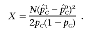 |
Similar to the  statistic, under the null hypothesis, X is distributed as the square of a standard normal distribution. With the true SNP frequencies denoted as p0C and p1C, and if pC=(p0C+p1C)/2, X is distributed under the alternative hypothesis as the square of a normal distribution with mean
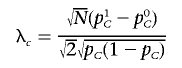 |
and variance ∼1, with the assumption that p0C≈p1C. The relation between λh and λc determines the relation between the power of  and X.
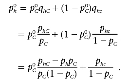
The underlying assumption in any indirect-association method is that the correlation structures of the cases and the controls are similar, as long as the two groups are sampled from the same underlying population. For instance, the underlying correlation structure is assumed to be similar to the closest HapMap population; therefore, the set of tag SNPs and the expected power of these SNPs to detect association can be estimated from the HapMap data set. More formally, we assume that the conditional probability qhC (or qhc) of haplotype h given C (or c) is the same in the case and control populations. If the cases and controls are sampled from a population that is similar to one of the HapMap populations, these conditional probabilities can be estimated from the HapMap quite efficiently, as we show in the “Estimating the Values  ” subsection.
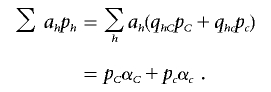
Under these assumptions, we have
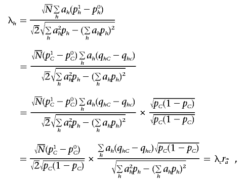 |
where
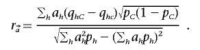 |
Thus, the power of detecting the causal SNP with a sample size of N individuals (with use of the χ2 statistic) is the same as the power of detecting the causal SNP with  individuals with use of the
  statistic. When the indirect-association method is performed on one SNP (i.e., m=1),
  is
is  , regardless of the weight vector
  . Thus,
  can be seen as a natural generalization to the standard notion of the r2 measure of LD.
Finding the Best Weight Vector
Clearly, it is desirable to perform the  test with a weight vector
  that maximizes
  . We now show that
  is maximized when ah is the conditional probability of C given h (denoted as qCh). That is, we show the following theorem.
Theorem 1: The power of the  statistic is maximized when, for each haplotype h, ah=qCh.
Proof: As shown above, the power of the  test is directly determined by the value of
  . We set
 |
and
 |
With these notations, the numerator can be written as  . If one assumes that for the optimal solution αC≠αc (otherwise, the optimum is zero, and then any vector
  will satisfy that
  ), it can be easily verified that, without loss of generality, we can arbitrarily choose the values of αC and αc, as long as they are nonnegative numbers. The latter follows from the fact that, if
  maximizes
  , then so does
  and
and  for every constant β. We thus set these values to satisfy
  and
and  .
.
The second term of the denominator can be written as
 |
At the same time, by the Cauchy-Schwartz inequality,
 |
where equality holds if there is a constant β, such that
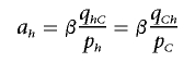 |
for every haplotype h. By adding the definition of αC and αc, we can satisfy this equality by setting β=pC. Put differently, the denominator is minimized when ah=qCh for every h. Since the numerator is now constant, the vector  maximizes the value of
  .
.
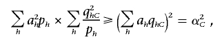
Note that, for the optimal selection of  —that is, when ah=qCh—we observe that
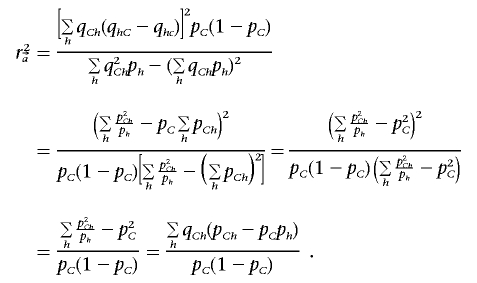 |
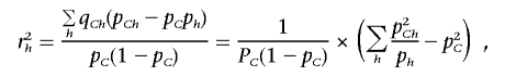
We denote, by
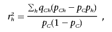 |
the correlation coefficient between the haplotype distribution of {h1,…,hk} and the causal SNP. It is easy to see that 0⩽r2h⩽1 and that r2h is always larger than the r2 coefficient between any group of haplotypes and the causal SNP; in particular, it is larger than the r2 coefficient between any single tag SNP and the causal SNP. Furthermore, when the number of SNPs used for the ρ test increases (i.e., m increases), the power of the association increases. To see this, consider the original haplotypes {h1,…,hk} and the haplotypes {h′1,h′′1,h′2,h′′2,…,h′k,h′′k} that are formed by adding one more SNP. By definition, pChi=pCh′i+pCh′′i, and phi=ph′i+ph′′i. Therefore, the r2h increases by
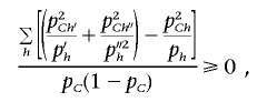 |
where the latter is true since (a+b)2/(c+d)⩽a2/c+b2/d for every four numbers a, b, c, and d > 0. Thus, increasing the number of SNPs can only amplify the power of detecting association with a hidden SNP. In practice, this is not exactly true, since the errors in the haplotype frequency estimates increase when the number of SNPs increases, and so does the effect of overfitting.
The ρ Test Compared with the χ2 Test
Since r2h is larger than the maximal r2 over all groups of haplotypes, we observe that the ρ test has more power than the χ2 test with 1 df applied to any single haplotype. A natural question is whether the ρ test is more powerful than the χ2 test with k-1 df when both statistics are applied to the set of haplotypes. This statistic can be written as
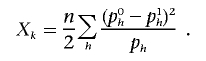 |
It is well known that, for the null distribution, Xk is distributed as χ2 with k-1 df. Now, we can write
 |
Therefore,
 |
Thus, we observe that
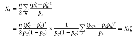 |
The last equality holds, since
 |
and, on the other hand,
 |
Under the alternative hypothesis, Xk is χ2k-1 distributed with mean λh, whereas the ρ test is χ21 distributed with mean λh. Therefore, one gains more power by using the ρ test. We note that this conclusion is valid under the assumptions made in this analysis and, in particular, under the assumption that, in the studied region, the disease is affected by one causal SNP. However, there are scenarios in which the statistic Xk has more power than the ρ test—for instance, when each of the different haplotypes affects the disease independently.
Estimating the Values 
Because Theorem 1 shows that the vector  , which maximizes the power of the ρ test, is
  , we are interested in estimating the values qCh from the HapMap population closest to the case and control populations.
To do so, we first estimate the haplotype frequencies over the set of SNPs s, s1,…,sm. The haplotype frequencies in a population can potentially be estimated by different methods, such as expectation maximization (EM)18 or PHASE.19 For our needs, we use HaploFreq,20 which is based on a likelihood model similar to the one used in the EM algorithm but which is probably more efficient and empirically more accurate than that in the EM algorithm. In particular, when whole-genome association studies are being performed, the efficiency of these algorithms is crucial, since every hidden SNP s requires a new calculation of the haplotype frequencies in the HapMap population.
Given the haplotype distribution over the entire set of SNPs, it is easy to calculate the values qCh by setting qCh=pCh/(pCh+pch). Since the frequencies pCh and pch are given by HaploFreq, we are able to calculate qCh.
Results
Benchmarks over HapMap ENCODE Regions
To evaluate the relative utility of our ρ test in comparison with single-SNP and multimarker methods, we performed several benchmarks, using the HapMap reference samples over the ENCODE regions. These data, from 270 individuals from four populations (people of European ancestry [CEU], Yoruba of Ibadan, Nigeria [YRI], Han Chinese [CHB], and Japanese [JPT]) are made up of polymorphisms over 10 genomic regions spanning a total 5 Mb of sequence. These regions have been carefully studied and are believed to have complete ascertainment for SNPs with frequency >5%. They are commonly used to estimate the performance of association statistics, since there are still many ungenotyped and unknown common SNPs in the rest of the genome.
In a typical association study, there is a set of marker SNPs (tag SNPs) that are genotyped and a set of SNPs that are not observed (hidden SNPs). To replicate this scenario, we used the intersection of SNPs from current genotyping platforms and SNPs from each of the ENCODE regions as our marker sets. Following the example of others,10,15 we measured the correlation between each SNP in the ENCODE regions with the best marker for the SNP from single tag SNPs (denoted as SNPs), multimarker tags (denoted as HAPs), and our WHAPs. We used the correlation coefficient r2 and r2h where appropriate, as measures of the utility of the various methods. Sets with a higher correlation have a greater potential power, since they are stronger proxies for the uncollected SNPs in the region.
The HAP and WHAP tags were selected by finding the strongest proxy via enumeration over all possible sets of two, three, and four tag SNPs within 100 kb of each SNP in every ENCODE region. We limited the tag length to four, to prevent overfitting (for a further examination of the issue of overfitting, see the “Robustness to Overfitting” subsection). We used two sets of tag SNPs for each ENCODE region: the SNPs contained in the Affymetrix 500k set and the SNPs contained in the Illumina HumanHap 550 set.
We compared the correlation coefficient of the WHAPs used for the ρ test with the correlation coefficient of a single SNP and a single HAP. Since the effective sample size is linearly related to the correlation coefficient, we measured the fraction of common SNPs (MAF ⩾5%) captured with a correlation coefficient larger than a given threshold, for a range of thresholds. Figure 2 demonstrates this performance evaluation over the sets of tag SNPs and the four HapMap populations. The figure demonstrates that the ρ test outperforms each of the other methods, in terms of correlation. Indeed, the ρ test has significantly higher correlation for every population on every platform at all thresholds. This is especially pronounced in populations with complex LD structure (e.g., YRI). Although the improvement shown by our simulations is only a modest one, we expect it to be more noticeable when haplotypes of more than four SNPs are used. As discussed below, this is currently prohibited because of the effects of overfitting, but larger reference data sets may allow such improvements in the future.
Figure 2. .

Fraction of SNPs captured by each of the methods tested on the Affymetrix 500k and Illumina HumanHap 550 marker sets. Shown is the fraction of SNPs with MAF ⩾5% that are captured by a marker SNP, HAP, or WHAP. The notion of a hidden SNP being captured depends on the r2 between the proxy and the SNP. For each graph, the X-axis represents the r2 threshold, and the Y-axis represents the fraction of common SNPs with r2 greater than the threshold. The three lines correspond to single SNPs, HAPs, and WHAPs. The populations are the four ENCODE panels: CEU, YRI, CHB, and JPT. Evidently, WHAPs significantly outperform both SNPs and HAPs over any platform and population but do especially well in populations with more-complex LD structure, such as YRI.
We explore the difference between HAPs and WHAPs by examining their relative increase in performance over single SNPs. We observe that both WHAPs and HAPs are significantly stronger proxies than SNPs. To elucidate their differences, tables 1 and 2 present the fraction of common SNPs captured with correlation coefficient ⩾0.8 and the average correlation coefficient. Evidently, the WHAPs are a much better proxy for the hidden SNPs than is the best HAP or the best tag SNP. In fact, we observe that the ρ test increases the correlation relative to the best HAP or SNP for 50.4% of the SNPs. In figure 3, we outline the distribution of weights for tags of these SNPs. Unfortunately, even though, in the majority of cases, the WHAPs serve as a better proxy than the best HAP or SNP, the average increase in r2 is modest, since the increase is >0.1 for 18.1% of the SNPs.
Table 1. .
Fraction of SNPs Captured by Each of the Methods[Note]
| Fraction ofSNPsa for |
||||
| Tag Set and Population |
SNP | HAP | WHAP | Increaseb (%) |
| Affymetrix 500k: | ||||
| CEU | .61 | .77 | .84 | 8.52 |
| CHB | .62 | .76 | .83 | 8.95 |
| JPT | .59 | .73 | .81 | 11.67 |
| YRI | .37 | .61 | .74 | 21.06 |
| Illumina HumanHap 550: | ||||
| CEU | .88 | .97 | .98 | 1.60 |
| CHB | .80 | .91 | .94 | 3.49 |
| JPT | .78 | .90 | .95 | 4.48 |
| YRI | .52 | .83 | .92 | 10.63 |
Note.— The highest fraction captured for each tag set and population is shown in bold type.
Fraction of common SNPs (MAF ⩾0.05) captured with r2⩾0.8 for each genotyping platform and population used in this study, with tags up to four SNPs in length. For each hidden SNP, the four tag SNPs were chosen from among all possible quartets of SNPs within 100 kb from the SNP.
Percentage increase in the fraction of captured SNPs when moving from HAPs to WHAPs. For example, the first row shows that, in the CEU population over the Affymetrix 500k chip, HAPs capture 77% of SNPs, whereas WHAPs capture 84% of the SNPs. This is an 8.52% increase in the number of captured SNPs. We prove that WHAPs always perform at least as well as HAPs in the “Material and Methods” section.
Table 2. .
Average r2 Obtained by the Different Methods[Note]
| Average r2 fora |
||||
| Tag Set and Population |
SNP | HAP | WHAP | Increaseb (%) |
| Affymetrix 500k: | ||||
| CEU | .77 | .87 | .91 | 4.37 |
| CHB | .75 | .86 | .91 | 4.96 |
| JPT | .74 | .85 | .90 | 5.88 |
| YRI | .59 | .79 | .87 | 9.17 |
| Illumina HumanHap 550: | ||||
| CEU | .92 | .97 | .99 | 1.26 |
| CHB | .86 | .95 | .97 | 2.42 |
| JPT | .86 | .94 | .97 | 2.77 |
| YRI | .71 | .91 | .96 | 4.84 |
Note.— The highest average correlation coefficient for each tag set and population is shown in bold type.
Average correlation coefficient for each genotyping platform and population used in this study with tags of up to four SNPs in length.
Percentage increase in the average correlation coefficient when moving from HAPs to WHAPs.
Figure 3. .

Histogram of the distribution of haplotype weights for SNPs, in which WHAPs provide a better proxy than a single HAP or a single SNP. The weight distribution was generated from the CEU population over ENCODE region ENm010.
Power Evaluation
Although correlation is important in determining the power of a method, other factors—such as frequency of a causal SNP, number of individuals, disease model, prevalence, relative risk, and multiple hypothesis correction—contribute to the overall power. To measure the increase in power in practice, we used the complete phased data for the ENCODE regions from the National Center for Biotechnology Information,21 to simulate panels of 1,000 cases and 1,000 controls with a disease prevalence of 0.01 and relative risk of 1.5. For each SNP with MAF ⩾0.05, we generated a panel in which the SNP is assumed to be the causal SNP. The total number of such panels was 32,017, corresponding to the number of SNPs with MAF ⩾0.05. We evaluated each statistic for these panels, using the tag SNPs from the Affymetrix 500k and Illumina HumanHap 550 SNP sets in each region. For the HAP and WHAP tests, for every hidden SNP in the region, we found the tags with maximum correlation to that SNP by enumerating over all possible subsets of SNPs within a window of 100 kb. We estimated P values, using a permutation test with 10,000 permutations to correct for multiple hypotheses. We consider a causal SNP as “identified” if its P value adjusted for multiple hypotheses is <.01. Table 3 presents the results of these power simulations. To illustrate the difference between the multimarker method and our WHAP method, the table presents the average relative power taken over all 10 ENCODE regions when compared with the ideal baseline situation in which we genotype every SNP. Comparing the power of these methods with the power of genotyping every SNP helps remove bias caused by factors such as differing MAFs, which are independent of the correlation coefficient. As expected from the results of the correlation coefficient experiment, we observe that our method outperforms the HAP method.
Table 3. .
Power Simulations
| Powerb of |
|||
| Tag Set and Populationa |
SNP | HAP | WHAP |
| Affymetrix 500k: | |||
| CEU | .92 | .94 | .96 |
| CHB | .90 | .94 | .95 |
| JPT | .90 | .93 | .95 |
| YRI | .77 | .88 | .92 |
| CEUh | .92 | .93 | .94 |
| CHBh | .90 | .91 | .91 |
| JPTh | .89 | .91 | .92 |
| YRIh | .77 | .87 | .90 |
| Illumina HumanHap550: | |||
| CEU | .98 | .98 | .99 |
| CHB | .95 | .97 | .98 |
| JPT | .96 | .97 | .99 |
| YRI | .86 | .95 | .96 |
| CEUh | .96 | .97 | .98 |
| JPTh | .96 | .96 | .96 |
| CHBh | .95 | .96 | .96 |
| YRIh | .87 | .95 | .95 |
For populations ending in “h,” haplotype weights were estimated using only half the individuals from the HapMap reference panel data, and power was measured using simulations over the other half.
Power of HAP and WHAP tests relative to genotyping all SNPs, averaging over all 10 ENCODE regions in simulated case-control studies of 1,000 cases and 1,000 controls. A relative risk of 1.5 is assumed.
Robustness to Overfitting
Our method is based on the assumption that the LD structure is consistent between the reference and case and control panels. There are several reasons why this may not be the case, and they have the potential of limiting the power of our method. First, it is not clear a priori whether the weights estimated from one population apply to another. To simulate discrepancies between the HapMap population and the case and control populations, we used the CHB genotype data to choose the best tags and to estimate the weights of haplotypes while measuring the power (using the ρ test) over simulations generated using the JPT population. For every hidden SNP in the region, we found the tags with maximum correlation to that SNP by enumerating over all possible subsets of SNPs within a window of 40 kb in the CHB population. With the Affymetrix 500k tags, the power of simulations that used the JPT population was 74%, 76%, and 78% for the best SNPs, HAPs, and WHAPs, respectively, obtained from the CHB population. With the Illumina HumanHap 550 tags, the power of simulations using the JPT population was 83%, 88%, and 89% for the best SNPs, HAPs, and WHAPs, respectively. Evidently, our method is not affected considerably by the difference in the population structure between the reference data set and the case and control populations.
Another complication may be the limited data size of the HapMap populations. Since the HapMap population is limited in size, there is the risk that the weights do not represent the true population haplotype frequencies but might instead be an artifact of overfitting. To measure the effect of overfitting on our results, we reestimated the haplotype frequencies, using only half the individuals in the HapMap panels, and then measured the power on the rest of the individuals with weights derived from the first half. As shown in table 3, these two error sources do not seem to considerably affect our method. If there was significant overfitting, we would expect power to drop significantly.
In addition, if there was significant overfitting, we would expect spurious correlation (high r2h values) between WHAPs and hidden SNPs because of the limited size of the HapMap populations. We measure the amount of spurious correlation by considering tag SNPs from all ENCODE regions as proxies for a random set of hidden SNPs from an ENCODE region on another chromosome. For each of the hidden SNPs, we found the best pair, triplet, and quartet of tag SNPs from other ENCODE regions and the corresponding haplotype weights. In all cases, no set of tag SNPs achieved an r2h>0.5, and the vast majority had very low r2h, which is evidence that our results are not due to overfitting.
Discussion
r2h and the ρ test can be used as a natural criterion for tag SNP selection, according to a similar argument for which r2 is currently used for tag SNP selection methods. Here, in contrast to previous methods, we suggest that the LD between a specific haplotype and the causal SNP not be used but that the LD between a weighted combination of the haplotype and the SNP be used instead.
In particular, our method has some similarities with the method proposed by Stram,17 in which the expectation of the hidden SNP is obtained from the haplotype frequencies with a block, and by Nicolae,16 who suggested a test similar to the ρ test. However, our approach differs from the methods presented by Stram,17,22 because we do not rely on haplotype blocks and instead use the multimarker tags that maximize the power of the indirect association (according to our analytic predictions), regardless of their location. Our approach also differs from the approach presented by Nicolae,16 since we formulate a much broader set of tests and show analytically that the maximum power is attained for the ρ test. Furthermore, our method for finding the set of WHAPs for every hidden SNP differs from the one suggested by Nicolae,16 and we show that this method is robust to overfitting and increases the power under simulations of association studies.
In this article, we focused on the optimization of haplotype-based tests for association studies when the set of genotyped SNPs (tag SNPs) is fixed. In cases where the tag SNPs are not fixed, it is also of interest to find a set of tag SNPs that will maximize the power of the study when the genotyping is followed by the haplotype analysis suggested here. The design of such a tag SNP selection algorithm is beyond the scope of this article, although it is likely that a greedy method, such as the one used for Tagger,10 would be a reasonable strategy to find such a set of SNPs. The software for performing association tests that use WHAPs can be downloaded from the WHAP Web site.
Acknowledgments
N.Z. is supported by the Microsoft Graduate Research Fellowship. N.Z. and E.E. are partially supported by National Science Foundation (NSF) grant 0513612 and National Institutes of Health grant 1K25HL080079. E.H. is supported by NSF grant IIS-0513599. H.M.K. is supported by the Samsung Scholarship. Part of this investigation was performed using the computing facility made possible by grants from the National Center for Research Resources, National Institutes of Health: the Research Facilities Improvement Program grant C06 RR017588, awarded to the Whitaker Biomedical Engineering Institute, and the Biomedical Technology Resource Centers Program grant P41 RR08605, awarded to the National Biomedical Computation Resource, University of California–San Diego. Additional computational resources were provided by the California Institute of Telecommunications and Information Technology (Calit2).
Web Resources
Accession numbers and URLs for data presented herein are as follows:
- WHAP, http://whap.cs.ucla.edu/
References
- 1.Devlin B, Risch N (1995) A comparison of linkage disequilibrium measures for fine-scale mapping. Genomics 29:311–322 10.1006/geno.1995.9003 [DOI] [PubMed] [Google Scholar]
- 2.Risch N, Merikangas K (1996) The future of genetic studies of complex human diseases. Science 273:1516–1517 10.1126/science.273.5281.1516 [DOI] [PubMed] [Google Scholar]
- 3.Collins FS, Brooks LD, Chakravarti A (1998) A DNA polymorphism discovery resource for research on human genetic variation. Genome Res 8:1229–1231 [DOI] [PubMed] [Google Scholar]
- 4.Matsuzaki H, Dong S, Loi H, Di X, Liu G, Hubbell E, Law J, Berntsen T, Chadha M, Hui H, et al (2004) Genotyping over 100,000 SNPs on a pair of oligonucleotide arrays. Nat Methods 1:109–111 10.1038/nmeth718 [DOI] [PubMed] [Google Scholar]
- 5.Gunderson KL, Steemers FJ, Lee G, Mendoza LG, Chee MS (2005) A genome-wide scalable SNP genotyping assay using microarray technology. Nat Genet 37:549–554 10.1038/ng1547 [DOI] [PubMed] [Google Scholar]
- 6.Johnson GC, Esposito L, Barratt BJ, Smith AN, Heward J, Di Genova G, Ueda H, Cordell HJ, Eaves IA, Dudbridge F, et al (2001) Haplotype tagging for the identification of common disease genes. Nat Genet 29:233–237 10.1038/ng1001-233 [DOI] [PubMed] [Google Scholar]
- 7.Pritchard JK, Przeworski M (2001) Linkage disequilibrium in humans: models and data. Am J Hum Genet 69:1–4 [DOI] [PMC free article] [PubMed] [Google Scholar]
- 8.Sham PC, Cherny SS, Purcell S, Hewitt JK (2000) Power of linkage versus association analysis of quantitative traits, by use of variance-components models, for sibship data. Am J Hum Genet 66:1616–1630 [DOI] [PMC free article] [PubMed] [Google Scholar]
- 9.The International HapMap Consortium (2005) A haplotype map of the human genome. Nature 437:1299–1320 10.1038/nature04226 [DOI] [PMC free article] [PubMed] [Google Scholar]
- 10.de Bakker PI, Yelensky R, Pe’er I, Gabriel SB, Daly MJ, Altshuler D (2005) Efficiency and power in genetic association studies. Nat Genet 37:1217–1223 10.1038/ng1669 [DOI] [PubMed] [Google Scholar]
- 11.Carlson CS, Eberle MA, Rieder MJ, Yi Q, Kruglyak L, Nickerson DA (2004) Selecting a maximally informative set of single-nucleotide polymorphisms for association analyses using linkage disequilibrium. Am J Hum Genet 74:106–120 [DOI] [PMC free article] [PubMed] [Google Scholar]
- 12.Chapman JM, Cooper JD, Todd JA, Clayton DG (2003) Detecting disease associations due to linkage disequilibrium using haplotype tags: a class of tests and the determinants of statistical power. Hum Hered 56:18–31 10.1159/000073729 [DOI] [PubMed] [Google Scholar]
- 13.Weale ME, Depondt C, MacDonald SJ, Smith A, Lai PS, Shorvon SD, Wood NW, Goldstein DB (2003) Selection and evaluation of tagging SNPs in the neuronal-sodium-channel gene SCN1A: implications for linkage-disequilibrium gene mapping. Am J Hum Genet 73:551–565 [DOI] [PMC free article] [PubMed] [Google Scholar]
- 14.Stram DO, Pearce C, Bretsky P, Freedman M, Hirschhorn J, Altshuler D, Kolonel L, Henderson B, Thomas DC (2003) Modeling and E-M estimation of haplotype-specific relative risks from genotype data for a case-control study of unrelated individuals. Hum Hered 55:179–190 10.1159/000073202 [DOI] [PubMed] [Google Scholar]
- 15.Pe’er I, de Bakker PI, Maller J, Yelensky R, Altshuler D, Daly MJ (2006) Evaluating and improving power in whole-genome association studies using fixed marker sets. Nat Genet 38:663–667 10.1038/ng1816 [DOI] [PubMed] [Google Scholar]
- 16.Nicolae DL (2006) Testing untyped alleles (TUNA)—applications to genome-wide association studies. Genet Epidemiol 30:718–727 10.1002/gepi.20182 [DOI] [PubMed] [Google Scholar]
- 17.Stram DO (2004) Tag SNP selection for association studies. Genet Epidemiol 27:365–374 10.1002/gepi.20028 [DOI] [PubMed] [Google Scholar]
- 18.Excoffier L, Slatkin M (1995) Maximum-likelihood estimation of molecular haplotype frequencies in a diploid population. Mol Biol Evol 12:921–927 [DOI] [PubMed] [Google Scholar]
- 19.Stephens M, Smith NJ, Donnelly P (2001) A new statistical method for haplotype reconstruction from population data. Am J Hum Genet 68:978–989 [DOI] [PMC free article] [PubMed] [Google Scholar]
- 20.Halperin E, Hazan E (2006) HAPLOFREQ—estimating haplotype frequencies efficiently. J Comput Biol 13:481–500 10.1089/cmb.2006.13.481 [DOI] [PubMed] [Google Scholar]
- 21.Zaitlen NA, Kang HM, Feolo ML, Sherry ST, Halperin E, Eskin E (2005) Inference and analysis of haplotypes from combined genotyping studies deposited in dbSNP. Genome Res 15:1594–1600 10.1101/gr.4297805 [DOI] [PMC free article] [PubMed] [Google Scholar]
- 22.Wang H, Thomas DC, Pe’er I, Stram DO (2006) Optimal two-stage genotyping designs for genome-wide association scans. Genet Epidemiol 30:356–368 10.1002/gepi.20150 [DOI] [PubMed] [Google Scholar]