Association Mapping via Regularized Regression Analysis of Single-Nucleotide–Polymorphism Haplotypes in Variable-Sized Sliding Windows

Abstract

Large-scale haplotype association analysis, especially at the whole-genome level, is still a very challenging task without an optimal solution. In this study, we propose a new approach for haplotype association analysis that is based on a variable-sized sliding-window framework and employs regularized regression analysis to tackle the problem of multiple degrees of freedom in the haplotype test. Our method can handle a large number of haplotypes in association analyses more efficiently and effectively than do currently available approaches. We implement a procedure in which the maximum size of a sliding window is determined by local haplotype diversity and sample size, an attractive feature for large-scale haplotype analyses, such as a whole-genome scan, in which linkage disequilibrium patterns are expected to vary widely. We compare the performance of our method with that of three other methods—a test based on a single-nucleotide polymorphism, a cladistic analysis of haplotypes, and variable-length Markov chains—with use of both simulated and experimental data. By analyzing data sets simulated under different disease models, we demonstrate that our method consistently outperforms the other three methods, especially when the region under study has high haplotype diversity. Built on the regression analysis framework, our method can incorporate other risk-factor information into haplotype-based association analysis, which is becoming an increasingly necessary step for studying common disorders to which both genetic and environmental risk factors contribute.

Rapid improvements in high-throughput genotyping technologies have greatly reduced the cost of genomewide analyses and are resulting in a boom of large-scale genetic association studies of common disorders. Involving either a group of candidate genes or the whole genome, these studies employ single SNP-based linkage disequilibrium (LD) mapping to systematically evaluate the role of common genetic variants in the risk of developing various complex disorders. By approaching comprehensive coverage of common genetic variants, these studies have a statistical power for detecting genetic risk factors with moderate effects that is much improved over that of previous studies.¹ Meanwhile, the comprehensive coverage of common genetic variants has also greatly increased the number of polymorphisms that need to be tested within a study and thus poses a great challenge for statistical analysis. LD-based association analysis can be performed by analyzing either individual SNPs or multiple-SNP haplotypes. It is still debatable which of the two methods is more powerful for detecting common risk factors, and it is likely that one method will perform better than the other under certain disease models and certain LD patterns.^2–8 In practice, both single-SNP and multiple-SNP haplotype analyses are performed in genetic association studies.

Strategies for performing haplotype analyses are still the subject of active debate and research. One of the important issues is how many adjacent SNPs should be included simultaneously in a particular haplotype analysis. Early suggestions were to perform the haplotype analysis within regions of high LD, often referred to as “LD blocks,” where most of the genetic variation can be captured by a limited number of haplotypes.⁹ To undertake such an analysis, LD blocks need to be defined before haplotype association tests are performed within each predefined LD block. Although this approach is simple and offers an appealing concept, the definition of haplotype blocks can be problematic. Several different criteria have been proposed,^9–12 but it is still unclear which one is the most suitable. Frequently, the boundaries of LD blocks are not obvious. In addition, performance of haplotype analysis within predetermined LD blocks fails to consider possible correlations among LD blocks. Furthermore, it is almost inevitable that LD block–based haplotype analysis will result in “orphan” SNPs that fall outside any predetermined LD blocks and are therefore excluded from haplotype analysis. In such instances, the full information on genetic variability within a region will not be used in the haplotype analysis. Hence, the use of LD blocks as the fundamental units of association testing may not be the most efficient strategy for haplotype analyses.¹³

Another strategy for performing haplotype analyses is based on the sliding-window framework, in which several neighboring SNPs, together called a “window,” are included in a haplotype analysis, and such a window-based analysis is performed in a stepwise fashion across the region under study. Initial approaches to sliding window–based haplotype analyses employed windows of uniform size.^14–16 However, the determination of the fixed window size in such methods can be cause for concern. In theory, the optimal window size should be the one that results in a haplotype or haplotypes that maintain the highest LD with the genetic risk variant or variants to be detected. The optimal window size, therefore, should be influenced by the underlying LD pattern. Use of a fixed window size becomes more problematic when haplotype analyses are performed over a large genomic region or over the whole genome, where LD patterns are surely variable across the region. Therefore, it is impossible to predefine a single optimal window size for a sliding-window analysis of large-scale data.

Alternatively, sliding window–based haplotype analyses can be performed without fixing the window size. In this implementation, a range of window sizes are considered in the haplotype analysis. By analyzing both simulated and experimental data, Lin et al.¹⁷ argued that an exhaustive search of all the possible windows of SNPs at the genome level is not only computationally practical but also statistically sufficient for detection of common or rare genetic-risk alleles. However, such an exhaustive search followed by a massive correction for multiple testing inevitably caused a loss of power. In addition, given a fixed number of samples, the number of haplotype tests that can be afforded should be limited; hence, it is more reasonable that the maximum window size be determined on the basis of the local LD pattern and the available sample size, rather than being as large as the size of a big region (e.g., a chromosome) in the genome scan. Recently, Browning used variable-length Markov chains for association mapping,¹⁸ attempting to adapt haplotype analyses to the local LD pattern. The adaptation is made by inferring the structure of the graph that represents the variable-length Markov chains, and each merging edge of the inferred graph represents a cluster of haplotypes that will be tested for association with the disease. The number of tests is decreased if the inferred graph is parsimonious. During its merging (clustering) process, Browning’s method considers all the haplotypes of all lengths for a fixed set of SNPs in a region and uses a modified merging algorithm of Ron et al.¹⁹ to ensure that low-frequency haplotypes are continually merged and that the inferred graph is parsimonious. As a result, when the region under study exhibits a complex LD pattern (e.g., because of a high recombination rate) and thus contains many unique haplotypes (each with low frequency), the merging process of Browning’s method will tend to group a large number of unique haplotypes into a small number of haplotype clusters. The inferred graph, therefore, will contain a limited number of merging edges for association tests. Consequently, each resulting merging edge is likely to have high haplotype diversity and to fail to capture the true association between particular haplotype(s) and underlying disease risk allele(s).

Besides the issue of the number of SNPs to be considered in haplotype analyses, another challenge is how to handle the large number of haplotypes in association tests. Haplotype analyses are generally performed in two distinct ways. One is to test each haplotype by performing a series of 1-df tests, followed by a correction for multiple testing, usually Bonferroni correction. The other way is to analyze the whole set of haplotypes by performing a single multiple-df global test. However, for both approaches, the power of detection is seriously weakened because of either the massive correction for a large number of tests or the many degrees of freedom. Several approaches have been proposed to tackle this problem. One commonly employed approach is to ignore rare haplotypes by grouping them into a single pseudohaplotype and hence to reduce the total number of haplotypes to be tested. For this strategy to be applied, a frequency threshold to define rare haplotypes needs to be specified in advance, which is sometimes tricky to do in reality. Moreover, when all the rare haplotypes are lumped together, the risk association with any rare haplotype(s) is likely to be missed, and even if it is not missed, it is impossible to interpret the positive association of this heterogeneous group of rare haplotypes with the disease. Seltman et al.²⁰ suggested an alternative approach that involved performing a series of 1-df tests guided by the cladogram, followed by Bonferroni correction. However, the sequence of the tests suggested cannot be optimal in all cases. For example, in their 14 simulated models, multiple-df global tests took the lead in 7 models, whereas the sequential tests took the lead in 6 models. So, the improvement of the detection power offered by this approach is marginal. A third approach is to cluster haplotypes by their similarity. For example, Durrant et al.²¹ designed an allele frequency–based haplotype-similarity measure, used standard hierarchical clustering to group haplotypes, and accepted the haplotype partition with the smallest association P value. The haplotype clustering in such an approach is independent of disease status, which creates an opportunity to increase the detection power if disease status is used to guide the haplotype grouping. Another appealing approach, called the “penalized log-likelihood method,” is to force similar haplotypes to have similar estimated effects by imposing a penalty on similar haplotypes with different estimated coefficients.²² The objective function to minimize for estimating the coefficients is the sum of the squared error plus a weighted penalty. To apply this method, a suitable haplotype similarity measure has to be selected from multiple existing ones. Moreover, the slow estimation of coefficients makes it time consuming to apply the cross-validation method for determining the weight that makes a trade-off between the sum of squared error and the penalty.

In this article, we propose a new method for performing variable-sized sliding window–based haplotype analysis. First, at each testing position (i.e., the beginning position of a sliding window), we determined the maximum window size for the haplotype analysis on the basis of local haplotype diversity as well as sample size. Subsequently, a joint analysis of all the haplotypes of different lengths (up to the maximum window size) at the same beginning position was performed using a regularized regression method. Guided by the disease status, the regularized regression shrinks the effects of noninformative haplotypes to zero, and hence the effective degrees of freedom of the regularized regression model is greatly reduced. Since the joint analysis in our method not only takes account of the dependency among haplotypes but also makes effective use of their complementariness, it is more efficient in managing a large number of haplotypes and thus is more powerful in association detection than are approaches employing either a large number of single-haplotype–based tests or a conventional global test of all the haplotypes. We evaluated the performance of our method, in terms of the power to detect the presence of a genetic risk allele, by comparing it with the performance of a single SNP–based test, cladistic analysis of haplotypes²¹ in a fixed-sized sliding-window framework, and an association-mapping method based on variable-length Markov chains, which is in the haplotype-clustering framework and makes use of local LD pattern.¹⁸ We have demonstrated that our current method provides better performance than these three methods.

Methods

For simplicity of exposition, we assume that the genetic association study is performed for a case-control analysis of phase-known haplotype data (see the “Discussion” section for how to generalize to phase-unknown genotype data). Consider M unrelated case and control chromosomes, typed for L SNPs in a region. Denote X_ij∈{1,2}, i=1,…,M and j=1,…,L, as the allele configuration at SNP j in chromosome i, and denote y_i∈{0,1}, i=1,…,M, as the disease status of chromosome i.

In the sliding-window framework, a window is a set of neighboring SNPs. A window ϖ^s_l denotes the set of SNPs {s,s+1,…,s+l-1}. The haplotype in chromosome i, composed of SNPs in a window ϖ^s_l, is denoted X_iϖ^sl. The set of distinct haplotypes in a window ϖ^s_l is defined as {X_iϖ^sl|i=1,…,M}. A variable-sized window that begins with SNP s, denoted as Ω^s, is a collection of windows ϖ^s_l, with l ranging from 2 to k_s, where k_s is the largest k such that |∪^k_l=2{X_iϖ^sl|i=1,…,M}|⩽M/2. In other words, the maximum window size in our variable-sized window is based on the local haplotype diversity and the available sample size, and it is defined in such a way that the number of distinct haplotypes in a variable-sized window is, at most, half the number of observed chromosomes. We assume that n is the number of independent variables (i.e., unique haplotypes) that are included in the regression model, and m is the number of samples we are given. To accurately estimate the coefficients in the regression model, n should be upper bounded by a function of m. For an ordinary regression analysis that maximizes the likelihood (i.e., minimizes the sum of squared error), a rule of thumb for the ratio n:m is . For the l₁-norm regularized regression that we use, although there is no theoretical proof yet, it has been suggested that, for the ratio n:m, n⩽m. ²³ Under the assumption that phase-known haplotypes are given as input data, M chromosomes correspond to M/2 diploid individuals (i.e., m=M/2); we therefore choose M/2 as the maximum number of distinct haplotypes that can be accommodated in the regularized regression model.

Performing the Association Test in a Variable-Sized Window

For a given s∈{1,…,L-1}, suppose there are J distinct haplotypes in the variable-sized window Ω^s. In this article, we take account of the dependency and complementariness among the J haplotypes and test them in one model. We make use of the shrinkage techniques in the regression to deal with the problem of the many degrees of freedom. The main reason for turning to regression is its fast estimation of coefficients. Use of regression models instead of logistic regression models is not uncommon in practice.^24,25 To work with a regression model, we introduce a new variable y^*_i for each y_i, and the former can be interpreted as a true underlying continuous phenotype represented by the latter. In our experiments, y^*_i=1 when y_i=1, and y^*_i=-1 when y_i=0.

There are two steps in performing the association test in a variable-sized window. In step 1, we estimate the haplotype effect differences for the J haplotypes, using l₁-norm regularized regression, which is described below. Those haplotypes whose estimated effect difference (with respect to the reference haplotype) is not equal to zero are taken as informative haplotypes. If there are no informative haplotypes, we claim that there is no association between the haplotypes in the window and the disease of interest; otherwise, we proceed to the next step. In step 2, we test the statistical significance of the informative haplotypes selected in the first step by the F test. Below we describe how to make use of the generalized degrees of freedom (GDF) to correct the selection bias in the first step and to calculate an unbiased P value for association in each variable-sized window.

l₁-Norm Regularized Regression

Suppose there are J distinct haplotypes in the variable-sized window Ω^s. Let D^s_ij, i=1,…,M and j=1,…,J, be a {0,1} variable, representing whether chromosome i contains haplotype j. The regularized regression model is parameterized with β^s={β^s₀,β^s₁…,β^s_J}, where β^s₀ is the haplotype effect of a reference haplotype, which is one of the J haplotypes, but is unknown before the fitting of the model; β^s_j is the haplotype effect difference between the jth haplotype and the reference haplotype. Unlike ordinary regression that aims to minimize the sum of squared error () between y^* and its estimation, the regularized regression has the joint objective of using the simplest model to obtain the least squared error. There is a hyperparameter α_s that makes a trade-off between these two contradicting objectives. The l₁-norm regularized regression uses as the model-complexity measure and estimates β^s by minimizing . The second term in the objective function forces the l₁-norm regularized regression to use as small a number of haplotypes as possible to predict y^* accurately.²⁶ For a known α_s, β^s can be found using quadratic programming techniques that are computationally intensive; LARS²³ was proposed to estimate β^s in time similar to that of standard linear regression for a series of α. The model obtained with a given α_s is called “α_s-indexed,” and its corresponding parameters are represented as β^s(α_s). We decided on the best value of α_s (equivalently, the best value of β^s) by the adaptive model-selection method,²⁷ which was observed to perform better than cross-validation methods.²⁸

A central concept in the adaptive model-selection method²⁷ is the GDF.²⁹ For a general modeling procedure, such as regularized regression, which involves variable selection, the GDF is introduced to correct selection bias and to accurately measure the complexity of the model obtained. Those who are interested in the details of the GDF can refer to the work of Ye.²⁹ The adaptive model-selection method generalizes Akaike information criterion (AIC), one of the model selection criteria, to the extended AIC, where the degrees of freedom in AIC are replaced with the GDF. For the computational details of the GDF and the extended AIC, please see appendix A. To decide on the best value of α_s, the adaptive model-selection method chooses the α that minimizes the extended AIC. Denote the chosen α_s as .

Using the GDF to Calculate Unbiased P Values

The estimated haplotype-effect differences are now , j=1,…,J. Those haplotypes whose values are not equal to zero are selected as informative haplotypes. We test the disease-haplotype association by testing the statistical significance of the informative haplotypes, using the F test. Under the null hypothesis of no association between the disease and the haplotypes in the variable-sized window, all the haplotypes have no effect difference with respect to the reference haplotype. Hence, the sum of squared error of the null model is , where . Under the alternative hypothesis, all the noninformative haplotypes have the same effect as the reference haplotype, and all the informative haplotypes have different effect differences. Under the assumption that the indices of the informative haplotypes are t₁,…,t_G, the sum of squared error of the alternative model is , where . The alternative model is -indexed, and we denote its GDF as . The statistic³⁰ to test the significance of the contributions of the informative haplotypes is

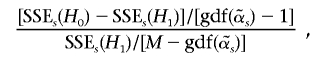which follows the F-distribution asymptotically under the null hypothesis, with the first degrees of freedom being and the second degrees of freedom being .

There are only G nonzero coefficients and one intercept in the alternative model; however, when the test statistic is calculated, the degrees of freedom of the alternative model are taken to be , which is usually >G+1. If we use G+1 as the degrees of freedom of the alternative model, the resulting P value will be biased downward. The GDF is used to correct the selection bias in the regularized regression²⁹; thus, the P value is called “unbiased” because it is calculated on the basis of the GDF of the model.

Simulation Data

All the simulation data were generated using the ms program.³¹ First, 4,000 haplotypes were generated using the following parameters: region size of 300 kb; effective population size of 10,000; recombination rate per site per generation of 10⁻⁹ or 10⁻⁷, and 300 SNPs within the region. Then, 2,000 individual samples were generated by randomly pairing the haplotypes. One or two SNPs with minor-allele frequency (MAF) of ∼0.05 were randomly selected as the disease-causing variant(s) from the region (see explanation below about the disease model). Under the assumption of a multiplicative model of disease inheritance and an equal case:control ratio, the phenotype of each individual was simulated using the logistic regression model (appendix B) and an odds ratio for the heterozygous genotypes at the causal SNP(s) in the range 1.2–2.5. After generation of the phenotypes, the genotypic information of the selected causal SNP(s) was removed from the simulated haplotypes before statistical analysis.

We simulated two types of data on the basis of two different disease models. In the first model, there is only one disease-causing SNP within the simulated region. In the second model, there are two disease-causing SNPs within the simulated region that act jointly (not interactively). When selecting the two risk SNPs within a region, in addition to the requirement that both SNPs have an MAF of ∼0.05, the pairwise r² between the two risk SNPs is required to be <0.1, and they are separated by as many SNPs as possible. The odds ratios for the two causal SNPs are set to be the same. Detailed simulation procedures are described in appendix B.

The decay of LD, seen in both D′ and r², in our simulated data (after filtering out the SNPs with MAF <0.03) was compared with that in the HapMap project.³⁴ The overall patterns of our simulated data (data not shown) are similar to those from the HapMap project.³⁴ Whereas the simulation data with a low recombination rate of 10⁻⁹ shows overall stronger LD and a slower LD decay than that of the HapMap data, the simulation data with a high recombination rate of 10⁻⁷ shows overall weaker LD and a faster LD decay than that of the HapMap data. Given the fact that the average recombination rate across 500 kb in the human ENCODE regions ranges from 0.19 to 1.25 cM,³⁴ the rate of 10⁻⁹ represents the low end of recombination rates in the human genome, whereas the rate of 10⁻⁷ represents a high recombination rate observed in some parts (hot spots) of the human genome. It is therefore expected that reasonable differences of LD pattern will be seen between our simulation data and the HapMap data, and our simulation data are suitable for evaluating the performance of our method for analyzing real human population data.

Experimental Data

Chinese subjects who received a diagnosis of idiopathic Parkinson disease from neurologists at two major movement disorder centers in Singapore (Singapore General Hospital and National Neuroscience Institute) were included in the study. The diagnosis of Parkinson disease was made in accordance with the diagnostic criteria of the United Kingdom Parkinson Disease Society Brain Bank. Healthy controls of similar age and matching sex and race were recruited at the same clinics. Institutional ethics committees approved the study, and informed consent was obtained from all study subjects.

Results

We compared the performance of our method of variable-sized sliding windows by use of regularized regression (referred to in the table and figures as “VSSWRR”) with three other methods for association analyses: allele-based single-locus χ² test (hereafter referred to as “SINGLE”), cladistic analysis of haplotypes²¹ (hereafter referred to as “CLADHC”), and association mapping by use of variable-length Markov chains¹⁸ (hereafter referred to as “VLMC”). SINGLE is used as a comparison baseline, CLADHC is used as a benchmark of haplotype analyses in a fixed-sized sliding-window framework; and VLMC is used as a benchmark of haplotype tests that are in the haplotype-clustering framework and make use of local LD pattern. Since CLADHC adopts a fixed window size, we analyze each replicate datum by using window sizes of 4–10 separately and present the highest power for each odds ratio. Throughout the article, we used Bonferroni correction to adjust for multiple testing (multiple sliding windows that start at different positions for our method, multiple haplotype partitions and multiple sliding windows for CLADHC, multiple single-SNP tests for SINGLE, and multiple haplotype cluster tests for VLMC).

Analysis of Simulated Data

For each of the two disease models, with a recombination rate per site per generation of 10⁻⁹, the simulation procedure in appendix B was invoked 100 times to generate 100 replicate data for each of the odds ratios: 1.2, 1.4, 1.6, 1.8, 2, and 2.5. To mimic a typical genetic association study, we first filtered out rare SNPs (MAF <0.03) and then identified tagging SNPs in 90 randomly selected individual samples (180 haplotypes), using a haplotype R² value of 0.85.³² On average, 18 SNPs remained after filtering by MAF and haplotype R². The phenotypes and tagging-SNP haplotypes of 2,000 simulated cases and simulated controls were subsequently used in genetic association analyses.

The performance comparisons among the four methods were done in two ways. First, the performance was evaluated in terms of the detection power—that is, the rate of declaring association on the basis of the smallest adjusted P value at a significance level of .05 within a region. Second, the performance was evaluated by calculating the type I error rate for each method, which was done by randomly permuting the disease status for each datum and then averaging over the disease models.

Our method consistently outperformed the other three methods in terms of the detection power at various odds ratios under the two different disease models. Under the single-disease-allele model (fig. 1), our method provides the best detection power among the four methods, although the difference between our method and VLMC (the second best) is moderate. At very low odds ratios (1.2–1.4), all the methods have poor power of detection, which is expected, given the low population frequency of the simulated disease allele and the limited size of the simulated sample of 1,000 cases and 1,000 controls. For moderate odds ratios (1.8–2.5), both our method and VLMC provide significantly higher detection power than do the CLADHC and SINGLE. Under the model of two disease alleles, for a moderate odds ratio (1.6–2), our method consistently provides 10%–20% more power than do the other three methods (fig. 2). All three haplotype-based methods perform better than SINGLE for odds ratios of 1.8–2.5; however, they do not perform better for low odds ratios—in this case, all the methods have poor detection power.

Figure 1. .

Comparison between methods of the detection power for the first type of disease model, in which disease status depends on one disease-causing SNP. Power is calculated under the assumption of a 5% experimentwise significance level, with Bonferroni correction for multiple testing. The recombination rate per site per generation in the simulated region is set to 10⁻⁹.

Figure 2. .

Comparison between methods of the detection power for the second type of disease model, in which disease status depends on two disease-causing SNPs in the observed region. The power is calculated under the assumption of a 5% experimentwise significance level, with Bonferroni correction for multiple testing. The recombination rate per site per generation in the simulated region is set to 10⁻⁹.

To further investigate the performance of each method, the haplotype complexity was increased by increasing the recombination rate per site per generation from 10⁻⁹ (fig. 2) to 10⁻⁷ (fig. 3) for the model of two disease alleles. With a recombination rate of 10⁻⁷, LD strength within the region under study was greatly reduced, and the haplotype complexity within the region therefore increased significantly. Specifically, for each of the 100 simulated data replicates, we calculated the number of unique haplotypes of length from 2 to L-s+1 (under the assumption that there are L SNPs) for each possible window beginning at position s. The average number of unique haplotypes over all s in the 100 simulation data increases from 94 to 1,760. The percentage of sliding windows that have >2,000 unique haplotypes of different lengths increases from 0% to 21%. For the region associated with high haplotype complexity (fig. 3), our method provides much better detection power than that of the other three methods, and ∼30%–50% more power than that of CLADHC, the second-best method. As the second-best method, CLADHC still performs significantly better than SINGLE and VLMC for odds ratios 1.8–2.5. Interestingly, VLMC, which is the second-best method for the simulated data with low haplotype complexity (a recombination rate per site per generation of 10⁻⁹), has the worst performance, with very poor detection power even for the high odds ratio of 2.5. Overall, the improved performance of our method compared with the other three methods is more significant in the region with high recombination rate and thus with high haplotype complexity.

Figure 3. .

Comparison between methods of the detection power for the second type of disease model, in which disease status depends on two disease-causing SNPs in the observed region. The power is calculated under the assumption of a 5% experimentwise significance level, with Bonferroni correction for multiple testing. The recombination rate per site per generation in the simulated region is set to 10⁻⁷.

We also compared the type I error rates of the four methods (table 1). Our method has the highest type I error rate; however, it is still below the nominal value of 5%, and the difference in the type I error rates between our method and the other three methods is moderate. This indicates that the significant improvement of our method in terms of detection power does not lead to a significant increase in the type I error rate or false-positive rate.

Table 1. .

Error Rates for Detection of Disease Association at the 5% Experimentwise Significance Level, Averaged over the Two Disease Models and Recombination Rates

Method	Type I Error Rate
VSSWRR	.032
SINGLE	.031
CLADHC	.011
VLMC	.031

Analysis of Experimental Data

We also evaluated the performance of the four methods by using experimental data generated in a genetic association study of Parkinson disease. The data include the genotypes of 96 SNPs (from a single candidate gene) obtained from 211 cases and 215 healthy controls. The most likely haplotype pair for each individual was inferred by PLEM.³³ Of 95 sliding windows, 81% have >426 (the number of total samples) unique haplotypes of different lengths. Among the four methods, only our method detected a significant association at the 5% experimentwise significance level after Bonferroni correction for multiple testing. The sliding window Ω³¹ (see the “Methods” section for description), beginning with SNP 31, had the smallest raw P value of .000285, which was significant after Bonferroni correction (fig. 4). The analysis was also performed using a permutation method for multiple-testing correction, and the conclusion remained the same. The smallest permutation-corrected P value of our method (for 1,000 permutations) was 0.019, whereas no significant evidence was detected by the other three methods (SINGLE and VLMC used 1,000 permutations, whereas CLADHC used 10,000 permutations because it involves two-level multiple testing). Within the sliding window of Ω³¹, the longest informative haplotype selected by the regularized regression has length 18; hence, the identified critical region of the putative risk allele(s) was from SNP 31 to SNP 48. To further evaluate the significance of this finding, we performed 100 cross-validation analyses. In each cross-validation, we randomly selected 174 cases and 176 controls from the whole sample. Since the sample size of the cross-validation analysis was only 350, the P values obtained were inevitably nonsignificant after multiple-window adjustment. However, of the 100 cross-validation analyses, 58 mapped the critical region of the putative risk alleles (defined by the longest informative haplotype) to the interval between SNPs 29 and 49, and 15 analyses mapped the critical region to the interval between SNPs 16 and 34, which overlapped with the original critical region determined in the whole sample. This suggested that the identified critical region of the putative risk allele was unlikely to be caused by sampling bias, although further validation analyses are warranted.

Figure 4. .

The −log₁₀ of raw P values obtained by our method for a single candidate gene for Parkinson disease. A total of 96 SNPs were typed for 211 cases and 216 controls. The horizontal line is the significance threshold obtained by Bonferroni correction at the experimentwise significance level of 5%. The X-axis shows the beginning position of each sliding window.

Discussion

In this article, we have proposed a haplotype-based method that works with variable-sized sliding windows to detect disease-haplotype associations for population-based case-control studies. For each variable-sized sliding window, the maximum window size is determined on the basis of local haplotype diversity as well as sample size. By doing a systematic performance evaluation under different disease models, we have shown that our method consistently outperforms the commonly used single-SNP–based association test and two haplotype association methods that have been demonstrated to be among the most effective methods to date. The outperformance of our method compared with the other three methods becomes much more significant when the region under study shows low LD. When the region under study exhibits extensive LD, our method provides good detection power (>60%) for disease alleles with moderate effects (odds ratio ⩾1.8) and a low population frequency of 5% and provides almost full power for the model of two disease alleles with odds ratio of 2.5 and a population allele frequency of 5%. Importantly, the improvement of detection power by our method does not lead to a significant increase in type I error rate, and the overall rate is well below the nominal value of 5%. Meanwhile, it is worth pointing out that, when the region under study has relatively low LD, the detection power of our method is still not optimal (<40%), although it performs much better than the other three methods. So, there is still space for further improvement on our method.

To our knowledge, our method is the first application of GDF and l₁-norm regularized regression to haplotype association analyses. A major challenge for haplotype association approaches is the large number of haplotypes to be tested, and the issue becomes even more challenging when an exhaustive analysis of haplotypes is performed. It is expected that, in an exhaustive analysis of haplotypes within a region, many haplotypes have the same prefix and are thus highly correlated (e.g., haplotypes 122, 1221, and 12212, all beginning with SNP s, are highly correlated). Meanwhile, because haplotypes may have complementary effects, considering one haplotype at a time will weaken association strength. A series of 1-df tests, followed by permutation-based multiple-testing adjustment, can take into account the dependency among the tests but ignores the complementariness among haplotypes. In contrast, the conventional single, multiple-df global test can take into account the complementariness but fails to consider the dependency among haplotypes, because it treats each haplotype as a totally independent identity. To account for the dependency among haplotypes, the penalized log-likelihood method²² introduced a penalty term to force similar haplotypes to have similar estimated effects. The regularized regression we adopted in this article behaves differently. The dependency among haplotypes is evaluated on the basis of disease status—that is, two haplotypes are considered to be highly redundant if the association of one haplotype with the disease is not much affected by consideration of the two haplotypes together. The regularized regression shrinks the effects of redundant haplotypes to zero, so that the effective degrees of freedom of the model are much smaller than the given sample size. Thanks to the fast estimation of coefficients in l₁-norm regularized regression, the best model (i.e., the best trade-off parameter) can be found by the adaptive model-selection method,²⁷ which was observed to be better than cross-validation methods.²⁸ By taking into account both the redundancy and the complementariness among haplotypes and by using the GDF technique, our regularized regression method provides a more efficient and effective way to analyze a large number of haplotypes in association test than performance of a series of 1-df tests or a single multiple-df global test.

For the first time, we implement a procedure in which the maximum window size of a sliding-window analysis is determined on the basis of local haplotype diversity and sample size. It is well known that, in a linear model, the number of covariates that can be accurately estimated is constrained by the number of observations or samples, although the method of constraining may be different for different model-building techniques. Given a fixed sample size, to ensure an accurate estimation of the model parameters, the number of covariates or unique haplotypes that can be considered should be limited. Unconstrained inclusion of a large number of haplotypes in association test will not increase but, instead, will decrease the detection power.

Our approach has better performance than CLADHC, which has been shown to be one of the most powerful approaches for haplotype analysis to date. The improvement of our approach over CLADHC can be reflected in several ways. First, our approach is based on variable sliding-window size, whereas CLADHC employs a fixed window size. As pointed out above, the employment of a fixed window size reduces the power for detecting risk haplotype(s). In our performance evaluation, multiple fixed window sizes were explored in CLADHC analysis, which is what is usually done in practice. The results of CLADHC should have undergone adjustment for multiple window sizes, and the performance of CLADHC would have been worse. Second, when the number of haplotypes in a window is large, CLADHC needs to first merge rare haplotypes into one category before hierarchical clustering is performed. In contrast, our method considers both common and rare haplotypes directly in the regularized regression model and can include rare haplotypes in the final model if they are statistically significantly associated with the disease of interest. Third, the haplotype partition in CLADHC is obtained by hierarchical clustering, which is greedy in nature. Hence, it is likely that the “best” haplotype partition identified is only suboptimal among all possible ones. To the contrary, the regularized sum of squared error that serves as the objective function in the regularized regression is globally minimized. Of course, CLADHC has its own advantage in terms of mapping disease susceptibility loci, because its hierarchical clustering is based on haplotype evolution to some extent. Another comparison is of computational efficiency. Within a sliding window, CLADHC tries different haplotype partitions and thus needs to adjust for multiple testing (multiple haplotype partitions) within a window, which is usually done by conservative Bonferroni correction. Alternatively, the adjustment can be done by a permutation approach, but it requires at least 1,000 permutations to get accurate adjusted P values, which is computationally intensive. Our method tests the association between the disease and all the haplotypes within a window in one model; hence, there is no need to do multiple-testing adjustment within a window. However, to calculate unbiased P values, our method does require a parametric bootstrapping procedure to estimate the GDF of the model built by the regularized regression. Fortunately, 100 bootstraps are usually enough to accurately estimate the GDF, which is much less computationally intensive than the permutation method for multiple-testing adjustment. In summary, our method outperforms CLADHC by enjoying the flexibility of window sizes and the effectiveness of managing a large number of both common and rare haplotypes.

Another unique feature of our method is that it takes into account the observed haplotype associations with the phenotypes of interest when the regression model is being built for testing. In contrast, CLADHC and VLMC first group haplotypes on the basis of haplotype similarity and then perform association tests. So, both of those methods do not consider the observed haplotype associations with phenotypes when grouping the haplotypes, although they take the haplotype evolution into account to some extent. Modeling haplotype evolution in association tests may give an easier biological interpretation of association evidence; however, a problem may be encountered when a region is analyzed for which either there is more than one disease-risk allele or both risk and protective alleles exist and these alleles have different evolutionary histories. The haplotype clustering–based method may also encounter a problem when the region under study exhibits a complex LD pattern and thus contains a large number of unique haplotypes. For example, the analyses of our simulation data indicated that VLMC grouped a larger number of unique haplotypes into a smaller number of haplotype clusters (merging edges in the fitted graph) in the region with a high recombination rate than in the region with a low recombination rate (data not shown). When a region with a large number of unique haplotypes is analyzed, the merging method of VLMC can result in a limited number of merging edges or haplotype clusters for testing, but the resulting haplotype clusters will become more heterogeneous and thus may fail to capture the true association between particular haplotype(s) and risk variant(s). This may explain, at least partially, the poor performance of VLMC under a high recombination rate. Therefore, the sequential nature (unsupervised haplotype grouping followed by association testing) of the existing haplotype clustering–based methods may be another reason why these methods have lower detection power than our method does.

There are, however, some limitations of our simulation analysis. First, our simulated data were constructed without the modeling of recombination hotspots. However, we did simulate the data by assuming a high or low recombination rate per site per generation (10⁻⁷ or 10⁻⁹). Given the observed range of the average recombination rate (0.19–1.25 cM) across 500 kb in the human ENCODE regions,³⁴ the rate of 10⁻⁹ represents the low end of recombination rates observed in the human genome, whereas 10⁻⁷ represents a high recombination rate observed in some parts (hotspots) of the human genome. The performance of our method in a region with recombination hotspots (a mixture of 10⁻⁷ and 10⁻⁹ recombination rates) is expected to be intermediate between the performances achieved with assumptions of low and high recombination rates across the whole region.

Second, we only simulated disease alleles with an MAF of 0.05. It is well known that the MAF of a disease allele has a major impact on the relative power of haplotype and single-marker methods. If there is only one common risk allele (MAF >0.05) within a region, it is likely that a single-marker test will have similar detection power as that of our haplotype analysis. However, when there is more than one common risk allele within a region, our method will have a better power than that of a single-marker analysis because association evidence from different haplotypes (associated with different risk alleles) may be built into a single regression model for testing in our method. For detecting disease-risk alleles with low MAFs, our method is likely to have even higher detection power than that of single-marker analyses and haplotype clustering–based approaches because our method includes directly the common and rare haplotypes in the regression model. By simulating a disease allele with low MAF and moderate effect, we explored a rather difficult scenario for detecting a risk allele to evaluate the power of our method.

Third, we directly simulated case and control samples instead of first simulating a source population and then randomly selecting cases and controls. Typical genetic association analyses are performed using cases and controls, often of similar numbers, that represent a very small proportion of the source population. Under the assumption of a relatively large sample size and a multifactorial disease model in which disease phenotype is influenced by multiple factors, each with a moderate effect, the random sampling of cases and controls from the source population should not cause a significant difference in LD pattern between the cases and the controls or between the selected samples and the source population. In our simulation data analysis, instead of simulating a source population and then a random sampling process, we directly simulated equal numbers of cases and controls that have a similar LD pattern and reflect the simulated disease model with a low disease-risk allele frequency and a moderate relative risk. By doing so, we eliminated the impact of a random sampling process. But, given the relatively large number of our simulated samples, they should be suitable for demonstrating the applicability of our method to real data.

Fourth, the use of Bonferroni correction for multiple-testing adjustment may impact the result of the power comparison between our method and the three competing methods, because Bonferroni correction overly penalizes a method that involves highly correlated tests. If one method involves a larger number of highly correlated tests, it will be overly penalized and therefore will appear to have a lower power than what would have been achieved if a more appropriate correction method (such as permutation-based correction) were used. Given that the sliding windows of our method are highly overlapping for adjacent SNPs, our method and SINGLE probably suffer a similar penalty from Bonferroni correction. As for VLMC, it is not clear whether the merging edges that are used for association testing suffer more from Bonferroni correction than do our variable-sized sliding windows; however, the type I error rates of VLMC and our method are very similar, suggesting that they are penalized to the similar degree. CLADHC may suffer more penalties than the other three methods do, because it needs to adjust for two-level multiple testing (one for multiple haplotype partitions within a window and the other for multiple windows). However, this could not be the sole reason why our method performed better than CLADHC, as we discussed above. The fact that the use of permutation tests in the analysis of the experimental data leads to the same conclusion as the use of Bonferroni correction suggests that our method might still have better power than the other three methods when permutation test is used for multiple-testing correction.

To mimic a typical genetic association study, our analysis of the simulated data was preceded by removal of rare variants and use of a tagging-SNP strategy; however, our regularized regression–based method can also be performed by consideration of all the typed SNPs. On one hand, including all the SNPs allows the full usage of genetic information and thus may increase the significance of the test within a sliding window. On the other hand, it also increases the total number of sliding windows and thus the total number of tests that need to be adjusted for. Currently, there is not a good solution to finding an optimal trade-off point between the maximization of genetic-information usage and the minimization of multiple-testing adjustment, because such a point seems to be different from case to case. For example, in our analysis of the candidate gene for Parkinson disease, use of all 96 typed SNPs allowed us to identify a significant association at the adjusted significance level of 0.05, whereas use of 15 tagging SNPs failed. One possible solution might be the application of the regularized regression to tests of the significance of all the informative haplotypes selected in all the sliding windows.

Our method can also be easily generalized to analysis of phase-unknown genotype data. For example, for phase-known haplotype data, D^s_ij in the regularized regression is an indicator of whether chromosome i contains haplotype j; for phase-unknown genotype data, D^s_ij can be set to the expected dosage of haplotype j in subject i.^35,36 In particular, D^s_ij can be the weighted average number of copies of haplotype j in the haplotype pairs that are compatible with the genotype of subject i, with the weights equal to the estimated haplotype frequencies. However, the simultaneous estimation of the haplotype frequencies and the haplotype effects in the regularized regression, as is done in a standard logistic regression,³⁷ needs further research. Our method works in a regression framework; hence, other risk factors can be incorporated as covariates in the regression model.

Our method has the potential to be applied to genomewide haplotype analysis, a very challenging task at the moment. Given the greatly varying LD patterns across the human genome, our variable-sized sliding-window method has a clear advantage over the methods that assume a fixed sliding-window size. Our method also has an advantage over the exhaustive haplotype analysis in a genomewide scan. In the genomewide analysis, the maximum window size of the exhaustive analysis can be as big as the whole chromosome. Consequently, the total number of unique haplotypes will be enormous, leading to a serious drain of power for detection. Our method overcomes this problem by determining the maximum window size on the basis of the local haplotype diversity and the sample size. In this study, we used the simple Bonferroni correction for the multiple-testing adjustment for different sliding windows, which is overly conservative, especially for a whole-genome analysis. Permutation-based adjustment is one alternative to multiple-testing adjustment. However, on the basis of our experience from this study, we think that the GDF is more favorable. Therefore, one future development will be to explore the application of the regularized regression and GDF to testing, in one model, the significance of all the informative haplotypes selected in all the sliding windows, for which a smaller number of parametric bootstrappings, rather than a large number of permutations, are performed.

The method for variable-sized sliding windows with use of regularized regression, coded in R, is available on request from the corresponding author.

Appendix A

In classical linear models, the number of covariates and the covariate identities are fixed, even if different observed responses are given; hence, the degrees of freedom are equal to the number of covariates. However, situations are different in the regularized regression. With α fixed but given slightly different observed responses, the regularized regression comes up with different β^s(α) values; as a result, the number of nonzero coefficients and the identities of the nonzero coefficients may be quite different. In other words, the α-indexed model found by the regularized regression may be instable, sensitive to small changes in the observed responses. Hence, the number of nonzero coefficients cannot accurately measure the model complexity any more—that is, the degrees of freedom of the α-indexed model are no longer equal to the number of nonzero coefficients in the model. For a general modeling procedure, such as the regularized regression, which involves variable selection, the GDF are introduced²⁹ to correct selection bias and to accurately measure the complexity of the model obtained. The GDF of a model is defined as the average sensitivity of the fitted values to a small change in the observed values. The parametric bootstrapping method proposed by Ye²⁹ estimated the GDF by perturbing the observed response a little bit in some way, estimating the response by use of perturbed data, and computing the ratio of the estimated response to the perturbation rate. Usually, 100 bootstrapping is enough to accurately estimate GDF; hence, it is relatively efficient.

Suppose the observed value y_i, i=1,…,n, is modeled as μ_i+ɛ, where μ_i is the expectation of y_i and ɛ is a Gaussian white noise with variance σ². An estimate s² for σ² can be obtained by an ordinary regression. Given a modeling procedure M:y→u, GDF(M), the GDF of the modeling procedure M, can be estimated as follows:

• 1. For t=1,…,T, first generate δ_ti∼normal(0,s²), i=1,…,n. Then, evaluate on the basis of the modeling procedure M.
• 2. Calculate as the regression slope from .
• 3. 

The estimation of GDF is relatively insensitive to the choice of s for s∈[0.5σ,σ].

Given GDF(M), the extended AIC is defined as .

Appendix B

The procedure that we used to generate the simulation data is as follows.

• 1. 
  Generate genotype data.

  • (a)
    Invoke the ms program³¹ to generate 4,000 chromosomes, with the required invoking parameters.
  • (b)
    Form genotype data by randomly pairing the haplotypes.
• 2. 
  Generate the phenotype (disease status).

  • (a)
    Randomly select the required number of disease-causing SNPs whose MAF is approximately the desired MAF.
  • (b)
    Generate the disease status based on the genotypes of the causal SNPs and the disease model by use of the following logistic regression model: , where I is the number of causal SNPs, OR is the specified odds ratio for the heterozygous genotype of the causal SNP, x_i is the 0-1-2 genotype coding for the ith causal SNP, and “constant” is a constant that renders the required case:control ratio.
• 3. Remove the genomic information for the selected causal SNPs from the simulated haplotypes.

References

- 1.Low YL, Wedren S, Liu J (2006) High-throughput genomic technology in research and clinical management of breast cancer: evolving landscape of genetic epidemiological studies. Breast Cancer Res 8:209 10.1186/bcr1511 [DOI] [PMC free article] [PubMed] [Google Scholar]
- 2.Barton NH (2000) Estimating multilocus linkage disequilibria. Heredity 84:373–389 10.1046/j.1365-2540.2000.00683.x [DOI] [PubMed] [Google Scholar]
- 3.Sevice SK, Lang DW, Freimer NB, Sandkuijl LA (1999) Linkage disequilibrium mapping disease genes by reconstruction of ancestral haplotypes in founder populations. Am J Hum Genet 64:1728–1738 [DOI] [PMC free article] [PubMed] [Google Scholar]
- 4.Maclean CJ, Martin RB, Sham PC, Wang H, Straub RE, Kendler KS (2000) The trimmed-haplotype test for linkage disequilibrium. Am J Hum Genet 66:1062–1075 [DOI] [PMC free article] [PubMed] [Google Scholar]
- 5.Zollner S, von Haeseler A (2000) Coalescent approach to study linkage disequilibrium between single-nucleotide polymorphisms. Am J Hum Genet 66:615–628 [DOI] [PMC free article] [PubMed] [Google Scholar]
- 6.Akey J, Li J, Xiong M (2001) Haplotypes vs single marker linkage disequilibrium tests: what do we gain? Eur J Hum Genet 9:291–300 10.1038/sj.ejhg.5200619 [DOI] [PubMed] [Google Scholar]
- 7.Morris RW, Kaplan NL (2002) On the advantage of haplotype analysis in the presence of multiple disease susceptibility alleles. Genet Epidemiol 23:221–233 10.1002/gepi.10200 [DOI] [PubMed] [Google Scholar]
- 8.Wessel J, Schork, N (2006) Generalized genomic distance-based regression methodology for multilocus association analysis. Am J Hum Genet 79:792–806 [DOI] [PMC free article] [PubMed] [Google Scholar]
- 9.Gabriel SB, Schaffner SF, Nguyen H, Moore JM, Roy J, Blumenstiel B, Higgins J, DeFelice M, Lochner A, Faggart M, et al (2002) The structure of haplotype blocks in the human genome. Science 296:2225–2229 10.1126/science.1069424 [DOI] [PubMed] [Google Scholar]
- 10.Daly MJ, Rioux JD, Schaffner SF, Hudson TJ, Lander ES (2001) High-resolution haplotype structure in the human genome. Nat Genet 29:229–232 10.1038/ng1001-229 [DOI] [PubMed] [Google Scholar]
- 11.Patil N, Berno AJ, Hinds DA, Barrett WA, Doshi JM, Hacher CR, Kartzer CR, Lee DH, Marjoribanks C, McDonough DP, et al (2001) Blocks of limited haplotype diversity revealed by high-resolution scanning of human chromosome 21. Science 294:1719–1723 10.1126/science.1065573 [DOI] [PubMed] [Google Scholar]
- 12.Zhang K, Deng M, Chen T, WatermanWS, Sun F (2002) A dynamic programming algorithm for haplotype block partitioning. Proc Natl Acad Sci USA 99:7335–7339 10.1073/pnas.102186799 [DOI] [PMC free article] [PubMed] [Google Scholar]
- 13.Zhao HG, Pfeiffer R, Gail MH (2003) Haplotype analysis in population genetics and association studies. Pharmacogenomics 4:171–178 10.1517/phgs.4.2.171.22636 [DOI] [PubMed] [Google Scholar]
- 14.Clayton D, Jones H (1999) Transmission disequilibrium tests for extended marker haplotypes. Am J Hum Genet 65:1161–1169 [DOI] [PMC free article] [PubMed] [Google Scholar]
- 15.Bourgain C, Genin E, Quesneville H, Clerget-Darpoux F (2000) Search for multifactorial disease susceptibility genes in founder populations. Ann Hum Genet 64:255–265 10.1046/j.1469-1809.2000.6430255.x [DOI] [PubMed] [Google Scholar]
- 16.Toivonen HT, Onkamo P, Vasko K, Ollikainen V, Sevon P, Mannila H, Herr M, Kere J (2000) Data mining applied to linkage disequilibrium mapping. Am J Hum Genet 67:133–145 [DOI] [PMC free article] [PubMed] [Google Scholar]
- 17.Lin S, Chakravarti A, Cutler DV (2004) Exhaustive allelic transmission disequilibrium tests as a new approach to genome-wide association studies. Nat Genet 36:1181–1188 10.1038/ng1457 [DOI] [PubMed] [Google Scholar]
- 18.Browning SR (2006) Multilocus association mapping using variable-length markov chains. Am J Hum Genet 78:903–913 [DOI] [PMC free article] [PubMed] [Google Scholar]
- 19.Ron D, Singer Y, Tishby N (1998) On the learnability and usage of acyclic probabilistic finite autommata. J Comput Syst Sci 56:133–152 10.1006/jcss.1997.1555 [DOI] [Google Scholar]
- 20.Seltman H, Roeder K, Devlin B (2001) Transmission disequilibrium test meets measured haplotype analysis: family-based association analysis guided by evolution of haplotypes. Am J Hum Genet 68:1250–1263 [DOI] [PMC free article] [PubMed] [Google Scholar]
- 21.Durrant C, Zondervan KT, Cardon LR, Hunt S, Deloukas P, Morris AP (2004) Linkage disequilibrium mapping via cladistic analysis of single-nucleotide polymorphism haplotypes. Am J Hum Genet 75:35–43 [DOI] [PMC free article] [PubMed] [Google Scholar]
- 22.Tanck M, Klerkx A, Jukema J, DeKnijff P, Kastelein J, Zwinderman A (2003) Estimation of multilocus haplotype effects using weighted penalized log-likelihood: analysis of five sequence variations at the cholesteryl ester transfer protein gene locus. Ann Hum Genet 67:175–184 10.1046/j.1469-1809.2003.00021.x [DOI] [PubMed] [Google Scholar]
- 23.Efron B, Hastie T, Johnstone I, Tibshirani R (2004) Least angle regression. Ann Stat 32:407–451 10.1214/009053604000000067 [DOI] [Google Scholar]
- 24.Molitor J, Marjoram P, Thomas D (2003) Fine scale mapping of disease genes with multiple mutations via spatial clustering techniques. Am J Hum Genet 73:1368–1384 [DOI] [PMC free article] [PubMed] [Google Scholar]
- 25.Albert JH, Chib S (1993) Bayesian analysis of binary and polychotomous response data. J Am Stat Assoc 88:669–679 10.2307/2290350 [DOI] [Google Scholar]
- 26.Hastie T, Tibshirani R, Friedman J (2001) The elements of statistical learning; data mining, inference, and prediction. Springer, New York [Google Scholar]
- 27.Shen AT, Ye JM (2002) Adaptive model selection. J Am Stat Assoc 97:210–221 10.1198/016214502753479356 [DOI] [Google Scholar]
- 28.Efron B (2004) The estimation of prediction error: covariance penalties and cross-validation. J Am Stat Assoc 99:619–632 10.1198/016214504000000692 [DOI] [Google Scholar]
- 29.Ye J (1998) On measuring and correcting the effects of data mining and model selection. J Am Stat Assoc 93:120–131 10.2307/2669609 [DOI] [Google Scholar]
- 30.Draper NR, Smith H (1980) Applied regression analysis. 2nd ed. Wiley, New York [Google Scholar]
- 31.Hudson RR (2002) Generating samples under a Wright-Fisher neutral model of genetic variation. Bioinformatics 18:337–338 10.1093/bioinformatics/18.2.337 [DOI] [PubMed] [Google Scholar]
- 32.Weale ME, Depondt C, Macdonald SJ, Smith A, Lai PS, Shorvon SD, Wood NW, Goldstein DB (2003) Selection and evaluation of tagging SNPs in the neuronal-sodium-channel gene SCN1A: implications for linkage-disequilibrium gene mapping. Am J Hum Genet 73:551–565 [DOI] [PMC free article] [PubMed] [Google Scholar]
- 33.Qin Z, Niu T, Liu JS (2002) Partition-ligation—expectation-maximization algorithm for haplotype inference with single-nucleotide polymorphisms. Am J Hum Genet 71:1242–1247 [DOI] [PMC free article] [PubMed] [Google Scholar]
- 34.The International HapMap Consortium (2005) A haplotype map of the human genome. Nature 437:1299–1320 10.1038/nature04226 [DOI] [PMC free article] [PubMed] [Google Scholar]
- 35.Stram DO, Haiman CA, Hirschhorn JN, Altshuler D, Kolonel L, Henderson BE, Pike MC (2003) Choosing haplotype-tagging snps based on unphased genotype data using a preliminary sample of unrelated subjects with an example from the multiethnic cohort study. Hum Hered 55:27–36 10.1159/000071807 [DOI] [PubMed] [Google Scholar]
- 36.Zaykin DV, Westfall PH, Young SS, KArnoub MA, Wagner M, Ehm MG (2002) Testing association of statistically inferred haplotypes with disease and continuous traits in samples of unrelated individuals. Hum Heredity 53:79–91 10.1159/000057986 [DOI] [PubMed] [Google Scholar]
- 37.Stram DO, Pearce CL, Bretsky P, Freedman M, Hirschhorn JN, Altshuler D, Kolonel LN, Henderson BE, Thomas DC (2003) Modeling and E-M estimation of haplotype-specific relative risks from genotype data for a case-control study of unrelated individuals. Hum Hered 55:179–190 10.1159/000073202 [DOI] [PubMed] [Google Scholar]