

Abstract
Genetic association studies offer an opportunity to find genetic variants underlying complex human diseases. The success of this approach depends on the linkage disequilibrium (LD) between markers and the disease variant(s) in a local region of the genome. Because, in the region with a disease mutation, the LD pattern among markers may differ between cases and controls, in some scenarios, it is useful to compare a measure of this LD, to map disease mutations. For example, using the composite correlation to characterize the LD among markers, Zaykin et al. recently suggested an “LD contrast” test and showed that it has high power under certain haplotype-driven disease models. Furthermore, it is likely that individual variants observed at different positions in a gene act jointly with each other to influence the phenotype, and the LD contrast test is also a useful method to detect such joint action. However, the LD among markers introduced by mutations and their joint action is usually confounded by background LD, which is measured at the population level, especially in a local region with disease mutations. Because the measures of LD that are usually used, such as the composite correlation, represent both effects, they may not be optimal for the purpose of detecting association when high background LD exists. Here, we describe a test that improves the LD contrast test by taking into account the background LD. Because the proposed test is developed in a regression framework, it is very flexible and can be extended to continuous traits and to incorporate covariates. Our simulation results demonstrate the validity and substantially higher power of the proposed method over current methods. Finally, we illustrate our new method by applying it to real data from the International Collaborative Study on Hypertension in Blacks.
Genetic association studies offer an opportunity to find genetic variants underlying complex human diseases.1 Currently, with the availability of large-scale genotyping techniques, genomewide association studies are underway. Nevertheless, the success of this approach relies on the linkage disequilibrium (LD) pattern between genetic markers, which are typically SNPs, and the functional mutations in a local region of the genome. It has been shown that LD patterns are quite variable in the genome.2–4
Various statistical methods have been developed to map functional variants. The most direct approach is single-marker analysis, which involves testing each SNP in turn for association with the disease. However, this simple approach may be inefficient, because any single marker may have limited information to predict the functional variant. Methods that can jointly make use of multiple marker information are therefore very useful. Multiple-marker association analysis may depend directly on either haplotypes or genotypes. Lack of parsimony is a major limitation of the multiple-marker approach, in which a large number of degrees of freedom is often involved in the test statistic. It is likely that there is no single uniformly optimal approach to mapping complex-disease genes.
Another approach is to contrast LD patterns between cases and controls because, in a local region that harbors the disease variant, the extent of LD may be different between cases and controls. For example, following the work of Nielson et al.,5 Zaykin et al.6 recently suggested a new “LD contrast test” to compare the pairwise matrices of disequilibrium measures between cases and controls. The use of composite coefficients to characterize the LD pattern in a local region allows their method to be robust to Hardy-Weinberg disequilibrium (HWD), which is expected to occur in the region with the disease variant. The LD contrast test was also suggested to test gene-gene interaction.7 The rationale behind this approach is that the joint effect of two variants would generate different LD patterns in cases and controls.
However, the LD between two SNP markers in a trait group, whether cases or controls, is the consequence of both selection on the basis of the disease variant and “background LD” due to various other factors. The use of the usual LD coefficients, which measure the whole correlation between two SNPs, may not be optimal for the purpose of detecting association, because of noise coming from the background LD. The most powerful measure for contrasting LD patterns must be able to discount appropriately the background LD. Therefore, it is desirable to find a new measure for capturing the local LD difference between cases and controls. Here, we propose a new test to overcome this problem. The proposed test is developed under a regression model and is flexible enough to incorporate covariates and continuous traits. Because the test depends directly on genotypes, it is also robust to HWD. Our simulation results demonstrate the validity and substantially improved power of this new test over the LD contrast test.
Methods
To illustrate the idea, we first consider a comparison of the LD for two SNPs between cases and controls. There is a variety of measures available to characterize LD in cases or controls. Following the notation of Zaykin et al.,6 the direct measure of the LD coefficient is given by
where PAB is the frequency of the haplotype with alleles A and B and where PA and PB are the frequencies of alleles A and B, respectively. It can be shown that DAB is related to the Pearson correlation coefficient by
 |
where PA1, PA2, PB1, and PB2 are the frequencies of the alleles 1 and 2 for markers A and B. A standardized measure, which is robust to allele frequency, is the coefficient D′AB,8 which is given by
 |
where
 |
This procedure restricts the range of D′ between 0 and 1. Complications in estimating the LD coefficients arise when only genotype data are observed. The estimates of both D′AB and DAB rely on the estimate of the haplotype frequency,  , which requires an assumption with regard to Hardy-Weinberg equilibrium. Because, in the local region with disease variants, deviation from Hardy-Weinberg proportions is expected in both cases and controls, Zaykin et al.6 suggested using composite LD measures, which are robust to HWD. Let PA/B be the joint frequency of alleles A and B in two different gametes, so that the composite LD coefficient is ΔAB=PAB+PA/B-2PAPB.9 We can see that composite LD coefficients do not distinguish between the two possible phases of the double heterozygotes but rather consider the deviation from random association. The composite correlation is given by
 |
where DA and DB are the HWD coefficients at the two loci—for example, at marker A, DA=p11-p21, in which p11 and p1 are the frequencies of genotype 11 and allele 1. The results of Zaykin et al.6 showed that tests based on composite correlations and composite LD coefficients have similar power.
Define the observed genotype value at the diallelic locus j for subject i as follows:
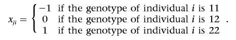 |
The composite correlation can then be estimated by
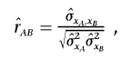 |
where, by denoting the sample means  and
and  ,
,  is the estimated covariance between the genotype values for loci A and B and
  and
and  are the estimated variances of the genotype values for loci A and B, respectively.10 Now, consider the sample mean–corrected, standardized genotype values zAi and zBi. Then, we can estimate the composite correlation by
 |
The statistic to compare the LD between cases and controls can be given by
where  and
and  are the estimated composite correlations between marker A and B in the case and control groups, respectively. Under the null hypothesis that no disease variant exists, TC is expected to be close to 0, so an unusually large or small TC statistic indicates the possibility of a disease variant.
Now, the statistic TC may be considered as equivalent to the regression coefficient in a regression model that has as dependent variable the cross-product of the standardized genotype values of two SNPs—that is,
where the predictor variable ti is an indicator variable for cases and controls and α and β are unknown parameters to be estimated. The parameter β describes the relationship between the predictor variable—in our example here, the case-control classification—and the correlation between two markers (i.e., LD), so a large or small observed value of the standardized estimate of β suggests association between the predictor (i.e., the trait) and two markers. The efficiency of the regression model (1) can be seen by considering the proportion of the dependent variable’s variance that is explained by the regression—that is, R2. It is useful to rewrite the dependent variable of model (1) as zAizBi=[(zAi+zBi)2-(zAi-zBi)2]/4, which shows that the dependent variable of regression model (1) is the special linear combination of the squared sum and squared difference of genotype values at two loci with equal weights. As discussed in the different context of Haseman-Elston regression to detect linkage,11–13 the test based on regression model (1) may not be efficient, because the background correlation is not taken into account. The efficiency of regression model (1) depends on the variance of the dependent variable explained by the trait status ti. Let us consider a class of dependent variables defined as all linear combinations of the squared sum and squared difference -w(zAi-zBi)2+(1-w)(zAi+zBi)2, where w is a weight, between 0 and 1. The most efficient such dependent variable should have the least overall variance. Let the variance of (zAi+zBi)2 be σ21, the variance of -(zAi-zBi)2 be σ22, and the covariance between (zAi+zBi)2 and -(zAi-zBi)2 be σ12. The optimal weight can be found by solving
 |
from which we find
 |
It can be seen that it is optimal for the squared sum and squared difference of genotype values at two loci to have equal weights when σ21=σ22. However, this is not expected to be the case, because of background correlation among the multiple markers in a local region. So, the composite correlation–based measure may lead to a severe loss in power.
The genotype value follows a multinomial distribution that is in the exponential family and therefore has the form eψ(xji,θji,φ), where j (j=A or B) denotes the marker and ψ(xji,θji,φ)=[xji-b(θji)]/d(φ)+c(xji,φ). Let random effects be denoted by bold letters. To improve the power of regression model (1), we consider modeling the genotype data as follows:
where h is a link function, xji represents the genotype value of marker j for the ith (i=1,…,n) subject, μj is the fixed overall intercept of the genotype value, uji is the marker intercept specific to individual i, and dji is the random effect of the trait on the specific genotype value. In this model, the genotype value of a marker for a subject is determined by overall mean μj, which may be looked at as the marginal allele frequency, the subject-specific effects uji, which lead to the LD observed in a general population, and the effect dji of the trait selection, which introduces the additional LD of interest. Under this model, the background LD is modeled by uji, and di=(dAi,dBi) is a random vector with mean 0 and covariance matrix modeled as
 |
where ϕ(ti) is a function of the trait values. Let  be the sample mean of the trait values, and define
  . Under this model, whether the correlation between markers (i.e., LD) is related to the trait value can be examined by testing H0:δ=0. We consider a canonical link function. The score statistic, which is the first derivative with respect to δ evaluated at the null hypothesis, is (see appendix A)
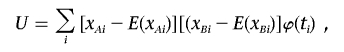 |
where xAi and xBi are the genotype values of two markers for individual i. Let μji=μj+uji. The mean E(xji)=b′(μji), in which j=A or B, depends on μji, which is unknown. So, we approximate the score statistic by using an estimate of the mean of xji,
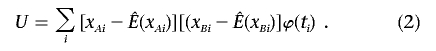 |
We note here that, when the genotype values are treated as constants,  , and, therefore, E(U)=0, so the validity of this statistic is not affected by the estimation of E(xji), regardless of the value of
  . However, the value of
  influences the power. There are several estimates available. One possibility is the sample mean of the genotype values over all subjects for each marker obtained by ignoring the background LD. For a case-control study with standardized genotype values, the statistic (2) is then equivalent to the composite correlation–based LD contrast test statistic. When the background LD is strong, the variation among individuals may be greater than the variation among markers within an individual, and, therefore, this test is not optimal in terms of power. To take into account the effect ui, we use a linear mixed model to estimate
  . Letting I be a vector of indicators for markers, which can also include appropriate covariates that we wish to adjust for, and βT be the corresponding row vector of regression coefficients, the model xji=βTI+ui+ɛji can be conveniently fitted using the lme function in the R package, which gives the best linear unbiased predictor (BLUP) of μji. Because the BLUP takes both types of information into account—the information across subjects and the information across markers—we expect it to improve the power of statistic (2). If there is concern over the sensitivity of the asymptotic distribution of this statistic, a simple permutation procedure that randomly shuffles the disease status can be adopted to determine the P value of the above statistic.
The new score statistic (2) is closely related to the composite correlation–based LD contrast statistic. It corresponds to testing β1=0 in the regression model E[(xAi-E(xAi)][(xBi-E(xBi)]=α1+β1ti, and so the parameter δ can be expressed as the regression parameter β1. The statistic TC is equivalent to testing the regression parameter β=0 in regression model (1). The dependent variables of both these regression models describe the correlation between two markers (the LD). Hence, both statistics detect association by testing whether the trait is related to the correlation between markers. However, with the aim of improving the power, the proposed statistic uses a different measure to describe this correlation, rather than using the conventional composite correlation. In the new statistic, the genotype values are centered by the individual specific means E(xAi) and E(xBi), which absorb background LD. So, the new test is in fact a test to compare “background-corrected LD” between cases and controls.
The comparison of the LD measure between cases and controls for only two SNPs can be directly extended to all pairwise LD statistics for a set of SNPs in a local region. Zaykin et al.6 showed, in their simulation, that the most powerful statistic is based on the overall difference of composite correlations between cases and controls, which is given by
where ΛY and ΛN are matrices of the composite correlations for cases and controls, respectively. Here, we define ΛY and ΛN such that each element is the corresponding sum of pairwise mean-corrected cross-products, by use of BLUPs of the means.
Results
Proof of Concept
As an initial proof of concept, we first provide evidence to show that discounting the background LD leads to increased efficiency of the test, in contrasting the LD patterns between cases and controls in the simplest case of only two SNP markers. We consider a situation in which two mutations independently occurred at a third (untyped trait) locus on haplotypes 00 and 11. In this case, the LD contrast test should have superior power over a single-marker analysis, because of the weak marginal effect of each marker, and also over a haplotype-based analysis, because of fewer degrees of freedom.5 First, four haplotype frequencies were determined by the allele frequencies and D′, and a pair of haplotypes randomly sampled from the corresponding multinomial distribution for each subject. The disease status is defined by a model similar to that used by Zaykin et al.6 For a dichotomous trait, the model assumes that the trait is due to an underlying continuous liability (y) to which the trait-locus effects (g) and random environmental effects (e) contribute additively and independently: y=g1+g2+e, where g1 and g2 are the trait-locus effects of the two haplotypes on an individual’s y value. The trait-locus effects are set to be 2.5 and 0.48 for haplotypes 00 (or 11) and 01 (or 10), respectively. Affection status is defined by a threshold Z, such that all individuals with y>Z are classified as cases. The random effect e is sampled from N(0,7.52). The prevalence is set to be 0.02. We consider sampling 100 cases and 100 controls. For each model, we simulate 1,000 data sets, and the permutation test is based on 1,000 replicates of each data set.
We first consider the influence of the background LD. We vary D′ from 0 to 0.8. To avoid any influence of the allele frequency, we choose the allele frequencies of both SNPs to be 0.5. Figure 1 shows the empirical power and type I error rate of three different tests for various values of background LD, including a test statistic in which  is estimated by the average genotype values of the two markers,
  (“D” in fig. 1). This statistic is equivalent to using the squared Euclidean distance between the genotype values of the markers as the dependent variable in regression model (1). Intuitively, when the background LD between two markers is high and the two markers have similar allele frequencies, this test is favored because the variability between markers is less than that among subjects. Otherwise, the correlation-based test is favored. The test proposed in this article that uses a mixed-correlation model to estimate the correlation of two markers is denoted “Mc” in the figures and should have high power when there is any background LD. We can see that all tests maintain good control of type I error rate at the 5% significance level (fig. 1, right). Figure 1 (left) shows that the power of the correlation-based test decreases with an increase in the background LD. As expected, we observe that the power profiles of the correlation- and distance-based tests cross each other, and the test that we propose is uniformly more powerful. Here, we show the results of the distance-based statistic only to illustrate that the background LD has a different impact on the various tests. When the markers have quite different allele frequencies, it is clear that the use of the average of different markers to predict μji is not suitable. We also evaluated the power under different prevalences, finding similar results. In figure 2, we assume that the quantitative phenotype values y—for example, for blood pressure—of cases and controls can be observed. Because the proposed statistic can make use of this quantitative information, it can further improve the power of the LD contrast test.
Figure 1. .

Comparison of the empirical power for 100 controls and 100 cases between the composite correlation–based LD contrast test (C), the proposed test (Mc), and the analogous statistic (D) in which the mean is estimated by the average genotype values of the two markers, at different background LD. The marker-allele frequencies of the two SNPs are both 0.5. The background LD is measured as D′.
Figure 2. .

Comparison of the empirical power and type I error rate for 100 controls and 100 cases between the composite correlation–based LD contrast test (C) and the proposed test (QMc) at different marker-allele frequencies when continuous phenotypes are observed. The background LD is D′.
Power
We further compare the power of tests for a set of markers with m SNPs in a local region or candidate gene. We also consider a single-marker analysis in the simulations, in which we fit the regression one marker at a time and the minimal P value (TP) is evaluated on the basis of a permutation procedure by shuffling the trait values to maintain the dependence among the markers. For multiple-marker analysis, we consider Hotelling’s TH, which jointly tests the marginal effects of multiple markers while accounting for the correlations among them.
The haplotypes for m=4 and 10 correlated SNP markers are simulated on the basis of a multivariate normal distribution with pairwise correlations ρ. Each allele of a haplotype is generated by dichotomizing the marginal normal distribution, and the cutoff is determined by an allele frequency that either is set to be between 0.1 and 0.5 or is randomly sampled from a uniform distribution between 0.1 and 0.5. The disease status is simulated as before, in which larger effects tend to be defined by haplotypes that are most different. In the power comparison, we consider three scenarios—that is, ρij is set to be a constant, is  , or is randomly sampled from a uniform distribution between 0.6 and 0.9. The scenario in which ρij equals a constant corresponds to an average pairwise correlation of 0.25 between SNPs, with each marker providing similar information about the disease locus. The scenario
  is similar to an LD pattern in which LD is primarily a function of marker distance. However, because of population phenomena such as genetic drift, mutation, nonrandom mating, and so forth, the actual LD pattern is more complicated; to simulate this last scenario, we sample ρ values from a uniform distribution between 0.6 and 0.9.
Here, we only show the results for m=4 markers because the results are quite similar for m=10 markers. The type I error rates for the four tests are all close to the nominal 0.05 level (data not shown). As seen in figure 3, for the case of multiple markers, we find results similar to those for the case of two markers. The proposed test usually performs better than the correlation-based test when background correlation exists among the SNPs, and the gain in power increases with increasing background LD. Figures 4 and 5 further show that the proposed test has uniformly the best performance compared with the other three tests in our simulations with two different LD patterns: LD as a function of marker distance and LD that does not necessarily follow the distances between pairs of markers. Because the LD contrast test detects different association information from that detected by TH and TP, as discussed by Zaykin et al.,6 and the marginal association information for each marker is small in our simulation, it is not surprising that we found much higher power for our statistic (figs. 4 and 5).
Figure 3. .

Comparison of the empirical power for 100 controls and 100 cases with four markers at different background LD (ρ) and allele frequencies (p) between the composite correlation–based LD contrast test (C), the proposed test (Mc), the minimum P value in single-marker analysis (minP), and Hotelling’s test of the marginal effects of multiple markers (H).
Figure 4. .

Comparison of the empirical power for 100 controls and 100 cases with four markers between the composite correlation–based LD contrast test (C), the proposed test (Mc), the minimum P value in single-marker analysis (minP), and Hotelling’s test of the marginal effects of multiple markers (H). The LD pattern is simulated to be a function of marker distance. The marker-allele frequency (p) is set to be 0.1–0.5 or is randomly sampled from a uniform distribution between 0.1 and 0.5.
Figure 5. .

Comparison of the empirical power for 100 controls and 100 cases with four markers between the composite correlation–based LD contrast test (C), the proposed test (Mc), the minimum P value in single-marker analysis (minP), and Hotelling’s test of the marginal effects of multiple markers (H). The ρ values are sampled from a uniform distribution between 0.6 and 0.9. The marker-allele frequency is set to be 0.1–0.5 or is randomly sampled from a uniform distribution between 0.1 and 0.5.
We further performed simulations based on the real LD pattern at the angiotension I–converting enzyme (ACE) locus (MIM 106180). The genotype data of 13 SNPs in the ACE locus for 310 independent subjects were selected from the Nigeria data set of the International Collaborative Study on Hypertension in Blacks.14 The LD pattern for the 13 SNPs at the ACE locus is given in figure 6. The squared correlation coefficient (r2) among SNPs is between 0 and 0.93, although most correlations among the SNPs are small. An underlying continuous liability value is similarly simulated as before, and a balanced case-control data set is determined by dichotomizing this continuous variable. The empirical power for the real LD pattern for the tests can been seen in figure 7, which shows that the proposed test is most powerful in the case of this real LD pattern.
Figure 6. .

The LD-pattern plot for 13 SNPs of the ACE locus. The color scale from white (lower values) to black (higher values) corresponds to an increase in the absolute values of correlation.
Figure 7. .

Comparison of the empirical power for 155 controls and 155 cases at different genetic effects between the composite correlation–based LD contrast test (C), the proposed test (Mc), the minimum P value in single-marker analysis (minP), and Hotelling’s test of the marginal effects of multiple markers (H). The LD pattern is from the real ACE genotype data of 310 subjects from Nigeria. The genetic effect (X-axis) is defined as the ratio of the genetic variance to the noise variance.
Application to Data on ACE Levels
The rennin-angiotensin system (RAS) is known to have a key role in blood-pressure regulation. ACE is a key component of the RAS because it catalyzes the conversion of angiotensin I to angiotensin II, a potent vasoconstrictor that leads to the constriction of blood vessels and the retention of salt and water. The ACE gene polymorphism has been extensively studied, although a causative effect of the ACE gene on hypertension is still not established.14–16 Bouzekri et al.17 described the association between 13 variants in the ACE gene at an average distance of 2 kb apart and the ACE plasma level in three population samples, from Nigeria, Jamaica, and an African American community in the United States. Their results suggest that there is more than one functional variant affecting the ACE plasma level. However, whether these variants affect the ACE plasma level interactively is unclear. To illustrate the application of our method, we tested whether the LD patterns of these 13 SNPs are different between subjects with higher and lower ACE plasma levels. We compare the new statistic (TMc) with two other LD contrast test statistics, in which the composite LD correlation (TC) and the standardized composite LD coefficient (TΔ′) are used to describe the LD pattern.
The data consist of 2,776 family members from Nigeria and Jamaica and an African American community. Our analysis is restricted to independent subjects with nonmissing genetic data from these families, by sampling one subject from each family. As a result, our analysis is based on 310 subjects from Nigeria, 116 subjects from Jamaica, and 252 subjects from the African American community. We further created a balanced case-control data set by equally dichotomizing the ACE level for each population. The P values for all tests were obtained using a permutation procedure with 500,000 replicates.
Table 1 presents the P values of the test statistics TMc, TC, and TΔ′ across the three population samples. In general, we consistently observed TMc and TC to have more power than TΔ′ in the three samples, whereas TMc also tends to show slightly stronger evidence of association than does TC, which is consistent with what we observed in the simulation studies.
Table 1. .
Results of Different LD Contrast Tests for the ACE Level and 13 Variants in the ACE Locus in Samples from Nigeria, Jamaica, and the United States
|
P |
||||
| Population | Sample Size | TMc | TC | TΔ′ |
| Nigerian | 310 | .0093 | .0689 | .6885 |
| Jamaican | 116 | .0020 | .0021 | .1902 |
| African American | 252 | .0738 | .0711 | .0742 |
Discussion
In the present study, we extend the LD contrast test under the framework of a generalized linear model. There are various analytic methods developed for a genetic association study. The LD contrast test relies on the difference of pairwise LD among markers, rather than on the change of the marginal allele frequencies. So, the LD contrast test and the single-marker or multiple-marker genotype score tests, such as Hotelling’s test, tend to detect different information available in the data. The genotype score–based tests are likely to fail in models in which there are no substantial marginal SNP effects. An example is seen when susceptibility haplotypes tend to be “yin-yang” haplotypes.18 There has been a report of an exceptional abundance of this particular haplotype pattern, in which two high-frequency haplotypes have different alleles at every SNP site (thus the name “yin-yang haplotypes”). The LD contrast is expected to have high power in this case. Haplotypes provide more information than do the allele frequencies and the pairwise LD. However, the haplotype-based tests often involve a large number of degrees of freedom. Because the LD extending more than two loci decays rapidly, it is reasonable to consider the allele frequencies and pairwise LD, rather than whole haplotypes, when the number of haplotypes is too large.
Currently, the LD contrast test depends on conventional LD measures, such as the composite correlation, to test whether there is a significant difference in these measures between cases and controls. One problem with the current method is that the LD introduced by trait selection is confounded by the background LD. Often, background LD is far greater than the trait-related LD in a local region of the genome. We show by simulations that the method proposed in this article can improve on the previous method by taking into account the background LD. However, the new test does not replace the LD contrast tests based on conventional LD measures. In practice, an investigator may be specifically interested in whether there is a significant difference in a conventional LD measure between cases and controls. In this case, the test with the corresponding LD measure, accompanying the graphical LD plots, is useful.
Our simulation studies suggest that the proposed test usually performs better than the correlation-based test when background correlation exists among SNPs. This can be further observed in the application of the method to ACE data in three population samples. The proposed method tends to detect the joint effects of SNPs. Therefore, it is understandable that we did not observe small P values in the original report, which focused on detecting the marginal effects.17 Our analysis here was restricted to independent subjects with nonmissing genetic data sampled from families. The sample sizes were thus much smaller than those used by Bouzekri et al.17 Both statistics TMc and TC consistently suggested an association between the ACE polymorphism and plasma ACE level. However, we found that the P values were above the 5% significance level for all the three test statistics in the African American sample (P=.073, P=.071, and P=.074 for TMc, TC, and TΔ′, respectively). The less significant results obtained from the African American sample might be because of its larger proportion of European ancestry, resulting in different background LD among the SNPs and therefore affecting the power.
Another feature of the proposed method is its flexibility. Our method can be used for both case-control and quantitative-trait data. When quantitative traits are observed, such as blood pressure or blood glucose level, the quantitative information of cases and controls can further improve the power of the method. Because the score statistic is derived under the framework of a generalized linear model, appropriate covariates, which can effectively control stratification effects that could otherwise invalidate a permutation test,19 can also be incorporated without difficulty into both the fixed and the random effects. To model pairwise LD, the genotype values of multiple markers are defined as correlated responses, and the trait value is defined as the predictor variable in the generalized linear model. The treatment of multiple markers in a cluster as a dependent variable has already been applied to association studies. Liang et al.20 applied generalized estimating equations for cluster genotype data. As an alternative, we use a mixed model to be able to separately model background LD and trait-related LD.
We have shown that the statistic TC, by directly comparing two correlation coefficients between cases and controls, is inefficient for detecting association when background LD is not negligible. It is well known that although valid statistics can be obtained that do not depend on correctly modeling the correlation structure, inappropriate specifications can result in a loss of efficiency. Direct comparison of two correlation coefficients is not optimal in terms of power, in that it does not take into account the correlation structure. The correlation can be looked at as a measure of the similarity between two variables. This argument is related to the more general statistical question of how to measure this similarity efficiently. A similar discussion can also be found among genetic linkage analyses, in which the similarity of trait and markers among family members is of interest.
Recently, Zhao et al.7 proposed to use the pairwise LD contrast to detect interaction between two loci. With the assumption that the two loci are unlinked, they showed that interaction between two loci indeed generates LD in the disease population and that the LD level generated by interaction depends on the magnitude of the interaction between the two loci. The method proposed in this article is a good complement to their method. Our method can improve the power because of the advantage that the BLUP has in making use of information both across subjects and across SNPs in each region. The proposed method should be especially useful when the LD contrast test is used to detect interaction among variants in LD, such as different variants in a candidate gene.21
The proposed method, just like other LD contrast tests, has limitations, as discussed by Zaykin et al.6 As found in our simulations, the LD contrast test will fail when the allele frequency is low. In this case, the primary association information exists in the difference between the marginal allele frequencies. A summary measure to capture both marginal effect and pairwise effect is desirable. We have found, in our study, that the pairwise Euclidean distance between genotype values among markers could be more powerful than other tests by simultaneously using both sources of information (data not shown). However, the gain in power of this measure depends on the unknown trait model. Further studies are needed to find a test that generally performs well under various reasonable models. In summary, we have improved the LD contrast test by taking into account the background LD. The new test is feasible for handling continuous traits and covariates.
Acknowledgments
We thank Dr. R. S. Cooper for permitting us to access the ACE data. This work was supported in part by a US Public Health Service Resource Grant from the National Center for Research Resources (RR03655), a Research Grant from the National Institute of General Medical Sciences (GM28356), a Cancer Center Support Grant from the National Cancer Institute (P30CAD43703), and a research grant from the National Human Genome Research Institute (HG003054).
Appendix A: Derivation of the Score Statistic
We derive the score statistic for testing H0:δ=0. The conditional likelihood function for subject i is
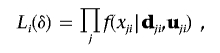 |
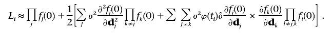
where j denotes the SNP in a cluster genotyped. For convenience of notation, we write f(xji|dji,uji) as f(dj), where dj is the trait related random effects for subject i. For simplicity, we omit the subject index i.The Taylor series expansion of L about dj=0 yields
 |
where j, k, and l denote different markers. Because the dj are not observed, we use the marginal likelihood by taking the expectation over dj:
 |
Let lj(dj)=log[fj(dj)]. We have
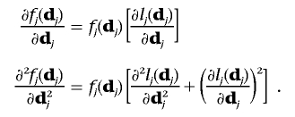 |
Then,
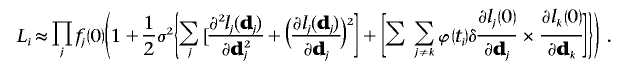 |
Assuming σ2 is known, the score statistic is the first derivative with respect to δ evaluated at the null hypothesis that there is no correlation introduced by trait values
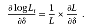 |
The likelihood function under the null hypothesis without the trait related random effect is L=jfj(0), and then
 |
If xji follows an exponential family distribution with a canonical link function, we have
 |
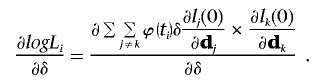
Then,
 |
For two SNP markers, the score statistic is then simply given by
 |
Without considering the background correlation induced by ui, E(xji) can be estimated by the sample mean. However, it is often not appropriate to simply omit the background correlation due to various factors, especially in a local region. In this case, we suggest estimating E(xji) by its BLUP.
Web Resource
The URL for data presented herein is as follows:
- Online Mendelian Inheritance in Man (OMIM), http://www.ncbi.nlm.nih.gov/Omim/ (for ACE locus)
References
- 1.Risch N, Merikangas K (1996) The future of genetic studies of complex human diseases. Science 273:1516–1517 10.1126/science.273.5281.1516 [DOI] [PubMed] [Google Scholar]
- 2.Daly MJ, Rioux JD, Schaffner SF, Hudson TJ, Lander ES (2001) High resolution haplotype structure in the human genome. Nat Genet 29:229–232 10.1038/ng1001-229 [DOI] [PubMed] [Google Scholar]
- 3.Reich DE, Cargill M, Bolk S, Ireland J, Sabeti PC, Richter DJ, Lavery T, Kouyoumjian R, Farhadian SF, Ward R, et al (2001) Linkage disequilibrium in the human genome. Nature 411:199–204 10.1038/35075590 [DOI] [PubMed] [Google Scholar]
- 4.Crawford DC, Carlson CS, Rieder MJ, Carrington DP, Yi Q, Smith JD, Eberle MA, Kruglyak L, Nickerson DA (2004) Haplotype diversity across 100 candidate genes for inflammation, lipid metabolism, and blood pressure regulation in two populations. Am J Hum Genet 74:610–622 [DOI] [PMC free article] [PubMed] [Google Scholar]
- 5.Nielsen DM, Ehm MG, Zaykin DV, Weir BS (2004) Effect of two and three-locus linkage disequilibrium on the power to detect marker/phenotype associations. Genetics 168:1029–1040 10.1534/genetics.103.022335 [DOI] [PMC free article] [PubMed] [Google Scholar]
- 6.Zaykin DV, Meng Z, Ehm MG (2006) Contrasting linkage-disequilibrium patterns between cases and controls as a novel association-mapping method. Am J Hum Genet 78:737–746 [DOI] [PMC free article] [PubMed] [Google Scholar]
- 7.Zhao J, Jin L, Xiong M (2006) Test for interaction between two unlinked loci. Am J Hum Genet 79:831–845 [DOI] [PMC free article] [PubMed] [Google Scholar]
- 8.Lewontin RC (1964) The interaction of selection and linkage. I. General considerations; heterotic models. Genetics 49:49–67 [DOI] [PMC free article] [PubMed] [Google Scholar]
- 9.Weir BS, Cockerham CC (1979) Estimation of linkage disequilibrium in randomly mating populations. Heredity 42:105–111 [DOI] [PubMed] [Google Scholar]
- 10.Zaykin DV (2004) Bounds and normalization of the composite linkage disequilibrium coefficient. Genet Epidemiol 27:252–257 10.1002/gepi.20015 [DOI] [PubMed] [Google Scholar]
- 11.Elston RC, Buxbaum S, Jacobs KB, Olson JM (2000) Haseman and Elston revisited. Genet Epidemiol 19:1–17 [DOI] [PubMed] [Google Scholar]
- 12.Xu X, Weiss S, Wei LJ (2000) A unified Haseman-Elston method for testing linkage with quantitative traits. Am J Hum Genet 67:1025–1028 [DOI] [PMC free article] [PubMed] [Google Scholar]
- 13.Wang T, Elston RC (2004) A modified revisited Haseman-Elston method to further improve power. Hum Hered 57:109–116 10.1159/000077548 [DOI] [PubMed] [Google Scholar]
- 14.Zhu X, McKenzie CA, Forrester T, Nickerson DA, Broeckel U, Schunkert H, Doering A, Jacob HJ, Cooper RS, Rieder MJ (2000) Localization of a small genomic region associated with elevated ACE. Am J Hum Genet 67:1144–1153 [DOI] [PMC free article] [PubMed] [Google Scholar]
- 15.Zhu X, Bouzekri N, Southam L, Cooper RS, Adeyemo A, McKenzie CA, Luke A, Chen G, Elston RC, Ward R (2001) Linkage and association analysis of angiotensin I-converting enzyme (ACE)-gene polymorphisms with ACE concentration and blood pressure. Am J Hum Genet 68:1139–1148 [DOI] [PMC free article] [PubMed] [Google Scholar]
- 16.Cox R, Bouzekri N, Martin S, Southam L, Hugill A, Golamaully M, Cooper R, Adeyemo A, Soubrier F, Ward R, et al (2002) Angiotensin-1-converting enzyme (ACE) plasma concentration is influenced by multiple ACE-linked quantitative trait nucleotides. Hum Mol Genet 11:2969–2977 10.1093/hmg/11.23.2969 [DOI] [PubMed] [Google Scholar]
- 17.Bouzekri N, Zhu X, Jiang Y, McKenzie CA, Luke A, Forrester T, Adeyemo A, Kan D, Farrall M, Anderson S, et al (2004) Angiotensin I-converting enzyme polymorphisms, ACE level and blood pressure among Nigerians, Jamaicans and African-Americans. Eur J Hum Genet 12:460–468 10.1038/sj.ejhg.5201166 [DOI] [PubMed] [Google Scholar]
- 18.Zhang J, Rowe WL, Clark AG, Buetow KH (2003) Genomewide distribution of high-frequency, completely mismatching SNP haplotype pairs observed to be common across human populations. Am J Hum Genet 73:1073–1081 [DOI] [PMC free article] [PubMed] [Google Scholar]
- 19.Chen HS, Zhu X, Zhao H, Zhang S (2003) Qualitative semi-parametric test for genetic associations in case-control designs under structured populations. Ann Hum Genet 67:250–264 10.1046/j.1469-1809.2003.00036.x [DOI] [PubMed] [Google Scholar]
- 20.Liang KY, Hsu FC, Beaty TH, Barnes KC (2001) Multipoint linkage-disequilibrium mapping approach based on the case-parent trio design. Am J Hum Genet 68:937–950 [DOI] [PMC free article] [PubMed] [Google Scholar]
- 21.Tao H, Cox DR, Frazer KA (2006) Allele-specific KRT1 expression is a complex trait. PLoS Genet 2:e93 10.1371/journal.pgen.0020093 [DOI] [PMC free article] [PubMed] [Google Scholar]