Bilinear dynamical systems

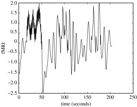
Abstract

In this paper, we propose the use of bilinear dynamical systems (BDS)s for model-based deconvolution of fMRI time-series. The importance of this work lies in being able to deconvolve haemodynamic time-series, in an informed way, to disclose the underlying neuronal activity. Being able to estimate neuronal responses in a particular brain region is fundamental for many models of functional integration and connectivity in the brain. BDSs comprise a stochastic bilinear neurodynamical model specified in discrete time, and a set of linear convolution kernels for the haemodynamics. We derive an expectation-maximization (EM) algorithm for parameter estimation, in which fMRI time-series are deconvolved in an E-step and model parameters are updated in an M-Step. We report preliminary results that focus on the assumed stochastic nature of the neurodynamic model and compare the method to Wiener deconvolution.

1. Introduction

Imaging neuroscientists have at their disposal a variety of imaging techniques for investigating human brain function (Frackowiak et al. 2003). The electroencephalogram (EEG) records electrical activity from electrodes placed on the scalp, the magnetoencephalogram (MEG) records the magnetic field from sensors placed just above the head, and functional magnetic resonance imaging (fMRI) records changes in magnetic resonances owing to variations in blood oxygenation. However, as the goal of brain imaging is to obtain information about the neuronal networks that support perceptual inference and cognition, one must first transform measurements from imaging devices into estimates of intracerebral electrical activity. Brain imaging methodologists are therefore faced with an inverse problem, ‘how can one make inferences about intracerebral neuronal processes given extracerebral/vascular measurements?’

Though not often expressed in this terminology, we argue that this problem is best formulated as a model-based spatio-temporal deconvolution problem. For EEG and MEG, the required deconvolution is primarily spatial, and for fMRI it is primarily temporal. Although one can make minimal assumptions about the source signals by applying ‘blind’ deconvolution methods (McKeown et al. 1998; Makeig et al. 2002), knowledge of the underlying physical processes can be used to great effect. This information can be implemented in a forward model that is inverted during deconvolution. In EEG/MEG, forward models make use of Maxwell's equations governing propagation of electromagnetic fields (Baillet et al. 2001), and in fMRI, forward models comprise haemodynamic processes as described by ‘Balloon’ models (Buxton et al. 1998; Friston 2002; Riera et al. 2004; Stephan et al. 2004).

In this paper, we propose a new state-space method (Haykin 1996) for model-based deconvolution of fMRI. The importance of this work lies in being able to deconvolve haemodynamic time-series, in an informed way, to disclose the underlying neuronal activity. Such estimates are required by many models of functional integration and connectivity in the brain. Typically, the influence of an experimental manipulation on the coupling between two regions is tested using a statistical model of the interaction between the experimental factor and neuronal activity in the source region. These interaction terms rest on being able to deconvolve the fMRI time-series. The procedures described below enable the construction of precise and informed interaction terms that can then be used to detect context-sensitive coupling among brain regions. The interaction terms are variously known as psychophysiological interactions (Friston et al. 1997), moderator variables in structural equation models (Buchel & Friston 1997) and bilinear inputs in dynamic causal models (Friston et al. 2003).

The model we propose is called a bilinear dynamical system (BDS) and comprises the following elements. Experimental manipulation (input) causes changes in neuronal activation (state), which in turn cause changes in fMRI signal (output). Experimental inputs fall into two classes: (i) driving inputs, which directly excite neurodynamics and (ii) modulatory inputs, which change the neurodynamics. These modulatory inputs typically correspond to instructional or attention set, and therefore allow neurodynamic changes to be directly attributed to changes in experimental context. Readers of our earlier papers on dynamic causal modelling (DCM; Friston et al. 2003; Penny et al. 2004) may well be experiencing a sense of ‘déjà vu’. This is no accident because BDS employs the same concepts of driving and modulatory inputs, neuronal states and outputs.

A key difference to DCM, however, is that BDS uses a stochastic neurodynamic model. This is biologically more realistic as regional dynamics are unlikely to be under full experimental control. Moreover, it has been established, across a variety of spatial scales, that neurodynamics can be meaningfully treated as stochastic processes, from Poisson processes describing spike generation (Dayan & Abbott 2001) to statistical mechanical treatments of activity in cortical macrocolumns (Ingber 1995). Stochastic components could also be considered as the consequence of local or global deterministic nonlinear dynamics of a possibly chaotic nature (see e.g. Breakspear & Terry 2002). From another perspective, stochastic components could be considered as reflecting input from remote regions (David & Friston 2003).

In BDS, neurodynamics cause changes in fMRI signals via haemodynamic models specified in terms of a set of basis functions. Although more detailed differential equation models exist (Buxton et al. 1998; Friston 2002; Riera et al. 2004), the relationship between neuronal activation and fMRI signals can be formulated as a first-order convolution with a kernel expansion using basis functions (typically two or three). This kernel is the haemodynamic response function. This approach has enjoyed a decade of empirical success in the guise of the general linear model (GLM; Friston et al. 1995; Henson 2003). Moreover, this means that the state-output relation can be described by a linear convolution.

The BDS model may be viewed as a marriage of two formulations, the input-state relation being a stochastic DCM and the state-output relation being a GLM.

BDS has a similar form to models used in signal processing and machine learning. In particular, BDS is almost identical to a linear dynamical system (LDS; Roweis & Ghahramani 1999) with inputs. The only difference is that the inputs can change the linear dynamics in a bilinear fashion—hence the name ‘bilinear’ dynamical systems. In such models, the hidden variable, which in our case corresponds to the neuronal time-series, can be estimated using Kalman smoothing. Furthermore, the parameters of the model can be estimated using an expectation-maximization (EM) algorithm (described in Ghahramani & Hinton 1996), which needs only minor modification to accommodate the bilinear term.

The structure of the paper is as follows. In §2 we define BDS and describe how it can be applied to deconvolve fMRI time-series. We describe a novel EM algorithm for estimation of model parameters. In §3 we present preliminary results on applying the models to synthetic data and data from an fMRI experiment.

(a) Notation

We denote matrices and vectors with bold upper case and bold lower case letters, respectively. All vectors are column vectors. X^T denotes the transpose of X, and I_k is the k-dimensional identity matrix. Brackets are used to denote entries in matrices/vectors. For example, A(i) denotes the ith row of A, A(i,j) denotes the scalar entry in the ith row and jth column, and a(i) denotes the ith entry in a. We define z_N as a vector with a 1 as the first entry, followed by N−1 zeros and 0_I,J as the zero matrix of dimension I×J.

2. Bilinear dynamical systems

Although, in principle, we could define models for activity in a network of regions, in this paper we define a BDS model for activity in only a single region. BDS is an input-state-output model where the states correspond to ‘neuronal’ activations. Neuronal activity is defined mathematically below, and can be thought of as that component of the local field potential to which fMRI is most sensitive (Logothetis et al. 2001). BDS is defined, for a single region, with the following state-space equations where n indexes time

$$s_n=(a+{\mathit{b}}^{\text{T}}{\mathit{u}}_n)s_{n-1}+{\mathit{d}}^{\text{T}}{\mathit{v}}_n+w_n$$ (2.1)

$${\mathit{x}}_n={[s_n,s_{n-1},s_{n-2},\dots ,s_{n-L+1}]}^{\text{T}}$$ (2.2)

$$y_n={\mathit{\beta }}^{\text{T}}\mathbf{\Phi }{\mathit{x}}_n+e_n$$ (2.3)

The first equation describes the stochastic neurodynamic model. Driving inputs v_n cause an increase in neuronal activity s_n (a scalar) that decays with a time constant determined by (a+b^Tu_n). This time constant is determined by the value of the ‘intrinsic connection’, a, and ‘modulatory inputs’, u_n. Driving inputs typically correspond to the presentation of experimental stimuli, and modulatory inputs typically correspond to instructional or attentional set. The strengths of the driving and modulatory effects are determined by the vectors of driving connections, d, and modulatory connections, b. The driving connections are also known as ‘input efficacies’. Neuronal activity is also governed by zero-mean additive Gaussian noise, w_n, having variance ${\sigma }_w^2$.

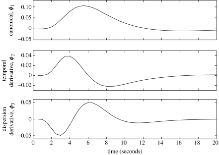
Neuronal activation then gives rise to fMRI time-series according to the second and third equations. The second equation defines an embedding process (Weigend & Gershenfeld 1994) in which neuronal activity over the last L time-steps is placed in the ‘buffer’, x_n. The vector x_n is referred to as an ‘embedded’ time-series, where L is the embedding dimension. Neuronal activation, now described by x_n, then gives rise to fMRI time-series, y_n, via a linear convolution process described in the third equation. Equation (2.3) comprises a signal term β^TΦx_n and a zero-mean Gaussian error term e_n with variance ${\sigma }_e^2$. The hth row of matrix Φ defines the hth convolution kernel (i.e. basis of the haemodynamics response function) and β(h) is the corresponding regression coefficient. Figure 1 shows a set of convolution kernels that have been used widely for the analysis of fMRI data in the context of the GLM. Linear combinations of these functions have been found, empirically, to account for most subject-to-subject and voxel-to-voxel variations in haemodynamic response (Henson et al. 2001; Henson 2003).

Figure 1.

Haemodynamic basis functions. Top panel: canonical function; middle panel: derivative of canonical with respect to time; bottom panel: derivative of canonical with respect to dispersion. Linear combinations of these functions have been found empirically to account for most subject-to-subject and voxel-to-voxel variations in haemodynamic responses (Henson et al. 2001; Henson 2003).

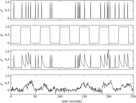
The model can perhaps be better understood by looking at the neuronal and haemodynamic time-series that it generates. An example is shown in figure 2. The model we have proposed, BDS, can be viewed as a combination of two models: (i) a stochastic, discrete-time version of DCM to describe neurodynamics and (ii) the GLM to describe haemodynamics. GLMs are well established in the neuroimaging literature (Frackowiak et al. 2003), and DCMs are becoming so. Consequently, the model choices we have made are informed by precedents established for GLMs and DCMs. For example, from previous work using GLMs (Henson et al. 2001), we know that the embedding dimension should be chosen to span a 20–30 s period. With regard to neurodynamics, the discrete bilinear form affords analytic tractability, while allowing nonlinear interactions between exogenous input and states. The splitting of exogenous inputs into driving and modulatory terms is also prompted by DCM. The motivation for this is that, for data collected from controlled experiments, one wishes to relate changes in connectivity to experimental manipulation. This distinction is echoed by the separate neurobiological mechanisms underlying driving versus modulatory activity (Penny et al. 2004).

Figure 2.

Time-series from exemplar BDS model. Driving input v_n (top panel) causes an increase in neuronal activity s_n (third panel). This activity decays with a time constant that changes according to a modulatory input u_n (second panel). In this instance, the modulatory coefficient, b, is negative. Driving inputs typically correspond to the presentation of experimental stimuli and modulatory inputs typically correspond to instructional or attentional set. Neuronal activity then gives rise to the fMRI time-series y_n (bottom panel) by convolving neuronal activity with a set of haemodynamic kernels (shown in figure 1).

The modulatory coefficients in equation (2.1), b, are also known as ‘bilinear’ terms. This is because the dependent variable, s_n, is linearly dependent on the product of s_n−1 and u_n. That u_n and s_n−1 combine in multiplicative fashion endows the model with ‘nonlinear’ dynamics that can be understood as a non-stationary linear system that changes according to experimental context. Importantly, because u_n is known, it is straightforward to estimate how the dynamics are changing. We emphasize that the term ‘bilinear’ relates to interactions between a state and an input rather than among the states themselves.

(a) Relation to biophysical models

In the previous section, we interpreted (a+b^Tu_n) as the time constant of decaying neuronal activity. However, our BDS model has a much more general relationship to underlying biophysical models of neuronal dynamics. Consider some biologically plausible model of neuronal activity that is formulated in continuous time $\dot{x}=f(x,\mathit{u},\mathit{\theta })$ and allows for arbitrarily complicated and nonlinear effects of the state and exogenous inputs. The parameters of this biophysical model θ (cf. neural mass models; Valdes et al. 1999) can be related directly to biophysical processes. In our discrete-time formulation, under local linearity assumptions, $a=\text{exp}(\mathrm{\Delta }t\partial f/\partial x)$ and $\mathit{b}(i)=\partial a/\partial \mathit{u}(i)=\mathrm{\Delta }ta{\partial }^{2}f/\partial x\partial \mathit{u}(i)$, where Δt is the sampling interval and i indexes the input. This means that our input-dependent autoregression coefficients can be regarded as a lumped representation of the underlying model parameters. This re-parametrization, in terms of a state-space model, precludes an explicit estimation of the original parameters. However, this does not cause concern, because we are not interested in the parameters per se; we only require the conditional estimates of the states. The transformation of a dynamic formulation into a discrete BDS is a useful perspective, because priors on the biophysical parameters can be used to specify priors on the autoregression coefficients, should they be needed.

(b) Relation to GLMs

For models with a single input, BDS reduces to a GLM if s_n=v_n, that is, if the neuronal activity is synonymous with the experimental manipulation (driving inputs). This highlights a key assumption of GLMs, that the dynamics of neuronal transients can be ignored.

For models with multiple inputs, the relation between BDS and GLMs is more complex. Ignoring bilinear and noise terms, BDS can be more parsimonious than the GLM, in the sense of having fewer parameters. Say, for example, we are modelling haemodynamics with H basis functions. Then for M (driving) input variables, the GLM has HM parameters, whereas in BDS, there are M+H+1 parameters. For H=3, for example, BDS has fewer coefficients if M is 3 or more.

The reason for this reduction is that, in BDS, the inputs affect only neurodynamics. And the strength of this effect, ignoring modulatory terms, is captured in a single parameter, the input efficacy. The relation between neurodynamics and haemodynamics is independent of which input excited neuronal activity. This is obviously more consistent with physiology, where experimental manipulation only affects fMRI by changing neuronal activity.

(c) Deconvolution

Deconvolution consists of estimating a neuronal time-series, s_n, given an fMRI time-series, y_n. It is possible to perform model-based deconvolution using BDS and a modified Kalman-filtering algorithm. The modification is necessary because, owing to the modulatory terms, the state transition matrix is time dependent. Also, the BDS model must be reformulated so that the output is an instantaneous function of the state. This section describes standard Kalman filtering and the modifications required for BDS.

In the Kalman-filtering approach, deconvolution progresses via iterative computation of the probability density $p(s_n|{\mathit{y}}_1^n)$, where ${\mathit{y}}_1^n=\{y_1,y_2,\dots ,y_n\}$. That is, our estimate of neuronal activity at time-step n is based on all the fMRI data up to time n (but not on future values).

The Kalman-filtering algorithm can be split into two steps that are applied recursively. The first step is a time update, where the density $p(s_{n-1}|{\mathit{y}}_1^{n-1})$ is updated to $p(s_n|{\mathit{y}}_1^{n-1})$. In our model this will take into account the effects of inputs u_n and v_n and the natural decay of neuronal activity. The second step is a measurement update, where the density $p(s_n|{\mathit{y}}_1^{n-1})$ is updated to $p(s_n|{\mathit{y}}_1^n)$, thereby taking into account the ‘new’ fMRI measurement y_n. The two steps together take us from time point n−1 to time point n, and are applied recursively to deconvolve the entire time-series.

A complication arises, however, because the Kalman filtering updates require that the output be an instantaneous function of the hidden state. That is, that y_n depend only on s_n and not on s_n−1, s_n−2, etc., which is clearly not the case. But Kalman filtering can proceed if we use the embedded state variables x_n. This will lead to an estimate of the multivariate density $p({\mathit{x}}_n|{\mathit{y}}_1^n)$. Our desired density, $p(s_n|{\mathit{y}}_1^n)$, is then just the first entry in $p({\mathit{x}}_n|{\mathit{y}}_1^n)$. While this is conceptually simple, a good deal of book-keeping is required to translate the BDS neurodynamical model into an ‘embedded space’. This is described in detail in appendices A and B.

A second complication arises in that, in the standard Kalman update formulae (Ghahramani & Hinton 1996), the inputs do not change the intrinsic dynamics. To account for this, we introduce a time-dependent state-transition matrix that embodies changes in intrinsic dynamics owing to modulatory inputs. This is also detailed in appendices A and B.

It is also possible to perform deconvolution based on Kalman smoothing rather than Kalman filtering. Kalman smoothing estimates neuronal activity, by computing the density $p(s_n|{\mathit{y}}_1^N)$. It is therefore based on the whole fMRI record, i.e. past and future values and, as we shall see, provides more accurate deconvolutions in high-noise environments.

(d) Estimation

To run the deconvolution algorithms described in the previous section, we must know the parameters of the model, e.g. β, a, b and d. If these parameters are unknown, as will nearly always be the case, they can be estimated using maximum-likelihood methods.

For BDS, this can be implemented using an EM algorithm, which we derive in appendices A and B. The E-step uses a Kalman-smoothing algorithm, which contains only minor modifications to the algorithm presented in Ghahramani & Hinton (1996). The M-step contains updates derived by considering estimation of the neurodynamic parameters (a, b, d) as a constrained linear regression problem (Rao & Toutenberg 1995). The neurodynamic parameters are updated as shown in equation (B 14), and the haemodynamic parameters, β, are updated using equation (B 17). It is also possible to update the initial state estimates as described in Ghahramani & Hinton (1996), but this was not implemented for the empirical work in this paper.

It is also possible to implement maximum-likelihood parameter estimation by computing the likelihood using Kalman filtering (as shown in Appendix C), and then maximizing this using standard Matlab optimization algorithms such as pseudo-Newton or Simplex methods (Press et al. 1992). However, preliminary simulations showed EM to be faster than these other maximum-likelihood methods.

(e) Initialization

The EM estimation algorithm is initialized as follows. In the limit of zero neuronal noise (ZNN), the neuronal activity is given by

$$s_n=(a+{\mathit{b}}^{\text{T}}{\mathit{u}}_n)s_{n-1}+{\mathit{d}}^{\text{T}}{\mathit{v}}_n,$$ (2.4)

and the predicted haemodynamic activity is

$${\hat{y}}_n={\mathit{\beta }}^{\text{T}}\mathbf{\Phi }{\mathit{x}}_n.$$ (2.5)

We initially set a random number between 0 and 1, and b such that b^Tu_n is between 0 and 1−a for all n. The values of d are also set to random numbers between 0 and 1. The first β coefficient is fixed at unity, and others, if there are any, are initialized to random numbers between 0 and 1. We then run a pseudo-Newton gradient descent optimization (the function fminunc in Matlab) to minimize the discrepancy between the observed fMRI time-series y_n and the estimated values ${\hat{y}}_n$ under the ZNN assumption. Occasionally, parameter estimates result in an unstable model. We therefore repeat these initialization steps until a stable model is returned. These parameters are then used as a starting point for EM.

3. Results

(a) Simulations

We generate simulated data to demonstrate various properties of the deconvolution algorithm. These simulations are similar to the first set of simulations in Gitelman et al. (2003). We also compare our results to those obtained with Wiener deconvolution (Glover 1999), which makes minimal assumptions about the source (that it has a flat spectral density; Press et al. 1992; Gitelman et al. 2003).

A 250 s time-series of input events with sampling period Δt=0.5 s was generated from a Poisson distribution, with a mean interval between events of 12 s. Events less than 2 s apart were then removed. The half-life of neuronal transients was fixed to 1 s by setting a=0.71, the input efficacy was set to d=0.9 and the neuronal noise variance was set to ${\sigma }_w^2=0.0001$. There were no modulatory coefficients, and a single haemodynamic basis function (the ‘canonical’, shown in figure 1) was used.

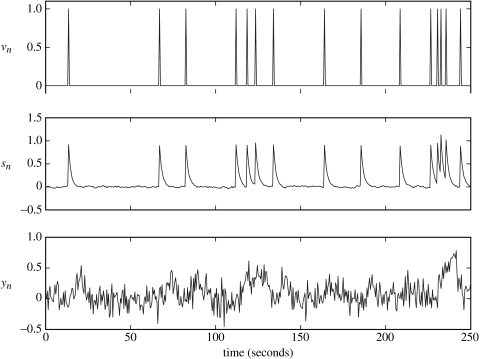
We then added observation noise to achieve a signal-to-noise ratio (SNR) of unity (this is equivalent to the 100% noise case in Gitelman et al. 2003). This was achieved using ${\sigma }_e^2=0.015$. The generated time-series is shown in figure 3.

Figure 3.

Low neuronal noise data. Top panel: driving input v_n; middle panel: neuronal activity s_n; bottom panel: fMRI data y_n.

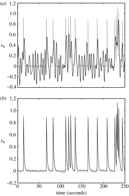
The parameters were estimated using EM to be a=0.72 and d=0.88. Wiener and BDS Kalman-smoothing deconvolutions (the latter obtained using estimated parameters) are shown in figure 4. Wiener deconvolution used the known value of ${\sigma }_e^2$, and BDS Kalman smoothing used the known values of ${\sigma }_e^2$ and ${\sigma }_w^2$. The quality of the BDS deconvolution is considerably better than that using the method described in Gitelman et al. (2003); see, for example, fig. 3D in Gitelman et al. (2003). This is because information about the paradigm (e.g. experimental inputs) has been used. For Wiener deconvolution, the correlation with the generated neuronal time-series is r=0.520 and for BDS Kalman smoothing it is r=0.998.

Figure 4.

Deconvolving low neuronal noise data. (a) Wiener deconvolution (solid line), (b) BDS Kalman-smoothing deconvolution (solid line) using estimated parameters a=0.72 and d=0.88. The simulated (true) neuronal activity is shown as a dotted line in both plots.

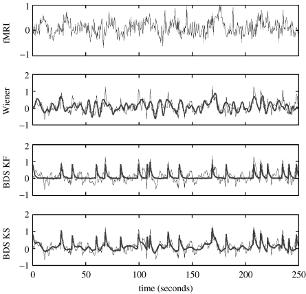
We then ran a second simulation with the neuronal noise variance set to a high value, ${\sigma }_w^2=0.03$. These data are shown in the top panel of figure 5. Neurodynamic parameters were estimated using EM to be a=0.68 and d=0.83. For comparison, ZNN initialization (see §2e) produced parameter estimates a=0.45 and d=1.13. That is, the assumption of ZNN leads to an underestimate of the neuronal time constant and an overestimate of the input efficacy.

Figure 5.

Deconvolving high neuronal noise data. Top (first) panel: fMRI data; second panel: Wiener deconvolution (thick line); third panel: BDS Kalman filtering (thick line); bottom (fourth) panel: BDS Kalman smoothing (thick line). In the bottom three panels, the original simulated neuronal activity is shown as a thin line. Wiener estimation recovers the intrinsic dynamics but misses the evoked responses (the ‘spikes’), whereas BDS Kalman filtering recovers the evoked responses but misses the intrinsic dynamics (slow fluctuations). Deconvolution using BDS Kalman smoothing recovers both.

The neuronal time-series, as estimated using BDS Kalman smoothing (bottom panel of figure 5), had a correlation with the generated time-series of r=0.775. The ZNN estimate neuronal time-series had a correlation of r=0.724. The Wiener deconvolved time-series (second panel in figure 5) gave r=0.52 (again). We also show, in the third panel of figure 5, deconvolutions from BDS Kalman filtering.

Figure 5 shows that Wiener estimation recovers the intrinsic dynamics but misses the evoked responses, whereas BDS Kalman filtering recovers the evoked responses but misses the intrinsic dynamics. Deconvolution using BDS Kalman smoothing recovers both.

The smoother can capture the intrinsic dynamics because it uses more information than the filter. It updates the filter estimates of neuronal activity, at a given time point, using information in advance of that time point (i.e. from the future). These updates are implemented using the ‘backward recursions’ described in Appendix B(a). Heuristically, the reason for the improvement is that the best estimates of neuronal activity are obtained using observed fMRI activity about 5 s or so in the future, i.e. at the peak of the haemodynamic response.

(b) Single word processing fMRI

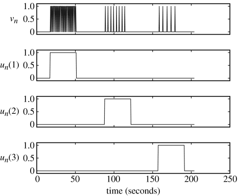
We now turn to the analysis of an fMRI dataset recorded during a passive listening task, using epochs of single words presented at different rates. The experimental inputs in figure 6 describe the paradigm in more detail. The driving inputs in the top panel indicate presentation of words in the subject's headphones and modulatory inputs in the lower panels indicate epochs with different presentation rates.

Figure 6.

Word fMRI inputs. Driving input v_n (top panel) and modulatory inputs u_n (lower panels). The delta functions in the top panel indicate presentation of words in the subject's headphones and the modulatory inputs in the lower panels indicate epochs with different presentation rates.

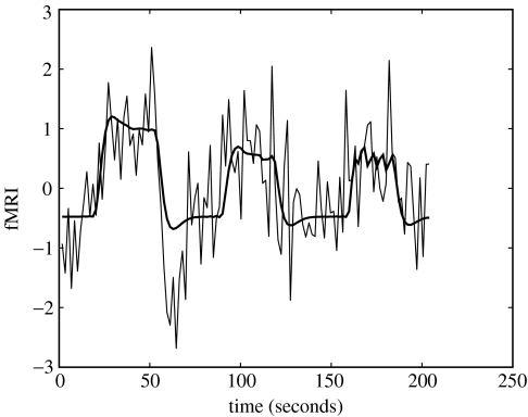
We focus on a single time-series in primary auditory cortex shown in figure 7. This comprises 120 time points with a sampling period Δt=1.7 s. Further details of data collection are given in Friston et al. (2003). As the experimental inputs are specified at a higher temporal resolution than the fMRI acquisition, we upsampled the fMRI data by a factor of 4 prior to analysis. The input variables were convolved with a ‘canonical’ haemodynamic response function (see top panel of figure 1) to form regressors in a GLM. Figure 7 shows the resulting GLM model fit.

Figure 7.

GLM fit to word fMRI data. fMRI time-series from primary auditory cortex (thin line) and GLM model fit (thick line).

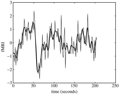
The same input variables and haemodynamic basis function were then used to define a BDS model. The observation and state noise variances were set to ${\sigma }_e^2={\sigma }_w^2=0.1$, and the haemodynamic regression coefficient was set to β=1. Figure 8 shows the resulting model fit which is clearly superior to the GLM model fit in figure 7 (but see §4). Figure 9 shows neuronal activity as estimated using BDS Kalman smoothing. This includes both event-related responses (the ‘spikes’) and intrinsic activity (slow fluctuations).

Figure 8.

BDS fit to word fMRI data. fMRI time-series from primary auditory cortex (thin line) and BDS model fit (thick line).

Figure 9.

BDS deconvolution of word fMRI data estimation of neuronal activity using BDS Kalman smoothing. Event-related responses can be seen as spikes superimposed on intrinsic dynamics.

Neurodynamic parameters were estimated using EM as d=0.80, a=0.92, b(1)=−0.44, b(2)=−0.08 and b(3)=−0.02. Thus, epochs with faster stimulus presentations were estimated to have an increasingly inhibitory effect on event-related neurodynamics. This pattern was robust across a wide range of settings of the noise variance parameters. This finding is consistent with neuronal repetition suppression effects and is in agreement with DCM of these data (Friston et al. 2003).

4. Discussion

We have proposed a new algorithm, based on a BDS, for model-based deconvolution of fMRI time-series. The importance of the work is that haemodynamic time-series can be deconvolved, in an informed way, to disclose the underlying neuronal activity. Being able to estimate neuronal responses in a particular brain region is fundamental for many models of functional integration and connectivity in the brain. Of course, these estimates can only describe those components of neuronal activity to which fMRI is sensitive. They should, nevertheless, be useful for making fMRI-based assessments of connectivity (Friston et al. 1997; Gitelman et al. 2003).

BDS is fitted to data using a novel EM algorithm where deconvolution is instantiated in an E-step and model parameters are updated in an M-step. Simulations showed EM to be faster than maximum-likelihood optimization based on simplex or pseudo-Newton methods. Deconvolution can be based either on a full E-step, using Kalman smoothing, or a partial E-step based on Kalman filtering. Kalman smoothing uses the full data record whereas Kalman filtering only uses information from the past.

Simulations showed that our model-based deconvolution is more accurate than blind deconvolution methods (Wiener filtering). This is because BDS uses information about the paradigm. We also observed the following trends. Wiener estimation recovers the intrinsic dynamics but misses the evoked responses, whereas BDS Kalman filtering recovers the evoked responses but misses the intrinsic dynamics. Deconvolution using BDS Kalman smoothing recovers both.

Simulations also suggest that if dynamics are indeed of a stochastic nature, as is assumed in BDS, then if we mistakenly assume deterministic dynamics, estimation of neuronal efficacies and time constants will become inaccurate. This has implications for models that assume deterministic dynamics, such as DCM (Friston et al. 2003).

Our applications of BDS provide good examples of Kalman smoothing providing better deconvolutions than Kalman filtering. The reason is that smoothing also uses future observations and the best estimates of neuronal activity are obtained using observed fMRI activity about 5 s or so into the future, that is, at the peak of the haemodynamic response. This property should hold for any state-space model of fMRI (see, for example, Riera et al. 2004).

A comparison of GLM and BDS model fits in figures 7 and 8 clearly shows that BDS is superior. Although this is somewhat encouraging, this observation should be tempered with a note of caution. This is because the BDS model is more complex and no penalty was paid for this during model fitting. The BDS model may therefore be overfitted. In particular, as fMRI time-series are known to contain aliased cardiac and respiratory artefacts, the finer details that BDS picks up may be of artefactual rather than neuronal origin. To eliminate this possibility one would need to estimate model parameters (especially the state noise variance) using Bayesian or cross-validation (Yamashita et al. 2004) methods. Fortunately, Bayesian methods have already been developed for linear dynamical systems (Ghahramani & Beal 2001) that should not require too many changes to accommodate the bilinear term.

Recently, Riera et al. (2004) have proposed a state-space model for fMRI time-series which allows for nonlinear state-output relations. They showed how model parameters could be estimated using a maximum-likelihood procedure based on extended Kalman filtering. Moreover, they showed how the parameters could be related to a stochastic differential equation implementation of the Balloon model. Thus, unlike BDS which assumes linear haemodynamics, their model can describe nonlinear properties such as haemodynamic refractoriness. This is important, as the neuronal refractoriness inferred using BDS in §3b, for example, may actually be of haemodynamic rather than neuronal origin. In fact, a DCM analysis of these data (Friston et al. 2003), which allows for both neuronal and haemodynamic refractoriness, concluded that both effects were present.

The model proposed by Riera et al. (2004) also differs from BDS in the input-state relations. In BDS, this is governed by driving inputs that excite linear neurodynamics, which can be changed according to modulatory inputs. This means that neurodynamics and changes in them can be directly attributed to changes in experimental context. This modelling approach is therefore appropriate for designed experiments where the inputs are known. In the Riera model, the inputs are not assumed to be known. Instead, a more flexible radial basis function approach is used to make inferences about the onsets of linear neurodynamical processes.

In previous work we have proposed an fMRI deconvolution model based on the GLM (Gitelman et al. 2003). This uses a forward model in which neuronal activity, represented using a temporal basis set and corresponding coefficients, is convolved with a known haemodynamic kernel to produce an fMRI time-series. Observation noise is then added. Deconvolution is achieved by estimating the coefficients of the temporal basis functions. In Gitelman et al. (2003), we used full-rank Fourier basis sets and overcomplete basis sets that used information about experimental design. Coefficients were estimated using priors and parametric empirical bayes. A problem with the method, however, is that for J coefficients (where J is typically the length of the time-series or longer) one must store and invert J×J covariance matrices. A computational benefit of the BDS approach is that, by making use of factorizations that derive from Markov properties of the state-space model, one need only manipulate L×L covariance matrices, where L is the temporal embedding dimension (L≪J). We have also argued, in §3b, that BDS is more parsimonious and biologically informed than the GLM.

The method we have proposed has been applied to deconvolve data at a single voxel. This is useful in providing a ‘source’ neuronal time-series, for example, for the analysis of psycho-physiological interaction (Friston et al. 1997; Gitelman et al. 2003). More generally, however, one is interested in making inferences about changes in connectivity in neural networks extended over multiple regions. This requires simultaneous deconvolution at multiple voxels and, ideally, a full model-based spatio-temporal deconvolution. The application of state-space models to this more difficult problem is an exciting area of current research (see, for example, Galka et al. in press).

Appendix A

Appendix A. Embedding

It is convenient to re-write the neurodynamic model as

$$s_n={\tilde{\mathit{b}}}^{\text{T}}{\tilde{\mathit{u}}}_n{s}_{n-1}+{\mathit{d}}^{\text{T}}{\mathit{v}}_n+w_n,$$ (A1)

and ${\tilde{\mathit{u}}}_n$ is a vector of modulatory inputs augmented with a 1 as the first entry (note some inputs may be driving and modulatory, in which case they appear in both ${\tilde{\mathit{u}}}_n$ and v_n) and ${\tilde{\mathit{b}}}^{\text{T}}={[a,\mathit{b}]}^{\text{T}}$ absorbs a.

The state-space equations can then be written in terms of the embedded neuronal activity, x_n, as

$$\begin{array}{l}{\mathit{x}}_n={\mathit{A}}_n{\mathit{x}}_{n-1}+\mathit{D}{\mathit{v}}_n+{\tilde{\mathit{w}}}_n\hfill \\ y_n={\mathit{c}}^{\text{T}}{\mathit{x}}_n+e_n,\hfill \end{array}\}$$ (A2)

where c^T=β^TΦ. The embedded state transition matrix is

$${\mathit{A}}_n=\left[\begin{array}{l}{\tilde{\mathit{b}}}^{\text{T}}{\mathit{F}}_n\hfill \\ {\mathbf{\Psi }}_L\hfill \end{array}\right],$$ (A3)

where

$${\mathit{F}}_n={\tilde{\mathit{u}}}_n{\mathit{z}}_L^{\text{T}}$$ (A4)

is a (B+1)×L matrix (where B is the number of modulatory inputs) and Ψ_L is the (L−1)×L delay matrix that fills the lower L−1 rows of A_n. This ensures that the embedded time-series are shifted one time-step each time A_n is applied. The input matrix is given by

$$\mathit{D}=\left[\begin{array}{l}{\mathit{d}}^{\text{T}}\hfill \\ {\mathbf{0}}_{L-1,M}\hfill \end{array}\right],$$ (A5)

where M is the number of driving inputs. The state noise in equation (A 2) is given by ${\tilde{\mathit{w}}}_n=w_n{\mathit{z}}_L^{\text{T}}$. The covariance of ${\tilde{\mathit{w}}}_n$ is Q and the only non-zero entry is $\mathit{Q}(1,1)={\sigma }_w^2$.

If we have a BDS with a single driving input, no modulatory inputs and L=4, a=0.92 and d=0.80, then the embedded neurodynamic model is

$${\mathit{x}}_n={\mathit{A}}_n{\mathit{x}}_{n-1}+\mathit{D}{\mathit{v}}_n+{\mathit{w}}_n$$ (A6)

$$\left[\begin{array}{l}{s}_n\hfill \\ s_{n-1}\hfill \\ s_{n-2}\hfill \\ s_{n-3}\hfill \end{array}\right]=\left[\begin{array}{llll}0.92\hfill & 0\hfill & 0\hfill & 0\hfill \\ 1\hfill & 0\hfill & 0\hfill & 0\hfill \\ 0\hfill & 1\hfill & 0\hfill & 0\hfill \\ 0\hfill & 0\hfill & 1\hfill & 0\hfill \end{array}\right]\left[\begin{array}{l}{s}_{n-1}\hfill \\ s_{n-2}\hfill \\ s_{n-3}\hfill \\ s_{n-4}\hfill \end{array}\right]+\left[\begin{array}{l}0.80\hfill \\ 0\hfill \\ 0\hfill \\ 0\hfill \end{array}\right]v_n+\left[\begin{array}{l}{w}_n\hfill \\ 0\hfill \\ 0\hfill \\ 0\hfill \end{array}\right].$$

Modulatory inputs would change the first entry in A_n.

Appendix B

Appendix B. EM algorithm

In probabilistic models with hidden variables, maximum-likelihood learning can be implemented using an EM algorithm (Dempster et al. 1977). This requires us to maximize the auxiliary function

$$F=\int p(\mathit{X}|\mathit{y})\text{log}p(\mathit{X},\mathit{y})\text{d}\mathit{X},$$ (B1)

where X={x₁,…,x_n,…,x_N} are the hidden variables and y={y₁,…,y_n,…,y_N} are the observed variables (Ghahramani & Hinton 1996). In BDS, the observed variables are the fMRI time-series and the hidden variables are the neuronal activities. Using the Markov property, we can write

$$p(\mathit{X},\mathit{y})=p({\mathit{x}}_1)\prod _{n=2}^{N}p({\mathit{x}}_n|{\mathit{x}}_{n-1})\prod _{n=1}^{N}p(y_n|{\mathit{x}}_n).$$ (B2)

The initial, transition and output probabilities are given by

$$p({\mathit{x}}_1)=N({\mathit{\mu }}_1,{\mathbf{\Sigma }}_1),$$ (B3)

$$p({\mathit{x}}_n|{\mathit{x}}_{n-1})=N({\mathit{A}}_n{\mathit{x}}_{n-1}+\mathit{D}{\mathit{v}}_n,\mathit{Q}),$$ (B4)

$$p(y_n|{\mathit{x}}_n)=N({\mathit{c}}^{\text{T}}{\mathit{x}}_n,{\sigma }_e^2),$$ (B5)

which define the observation model, state transition model and initial state distribution. In the above expression, the quantity c is as defined in equation (A 2). Therefore, the joint log-likelihood is a sum of quadratic terms

$$L_J=\text{log}p(\mathit{X},\mathit{y})=-\sum _{n=1}^N\frac{1}{2{\sigma }_e^2}[{(y_n-{\mathit{c}}^{\text{T}}{\mathit{x}}_n)}^{\text{T}}(y_n-{\mathit{c}}^{\text{T}}{\mathit{x}}_n)]-\frac{N}{2}\text{log}\left|{\sigma }_e^2\right|-\sum _{n=2}^N\frac{1}{2}[{({\mathit{x}}_n-{\mathit{A}}_n{\mathit{x}}_{n-1}-\mathit{D}{\mathit{v}}_n)}^{\text{T}}{\mathit{Q}}^{-1}({\mathit{x}}_n-{\mathit{A}}_n{\mathit{x}}_{n-1}-\mathit{D}{\mathit{v}}_n)]-\frac{1}{2}[{({\mathit{x}}_1-{\mathit{\mu }}_1)}^{\text{T}}{\mathbf{\Sigma }}_1^{-1}({\mathit{x}}_1-{\mathit{\mu }}_1)]-\frac{1}{2}\text{log}\left|{\mathbf{\Sigma }}_1\right|-\frac{N-1}{2}\text{log}\left|\mathit{Q}\right|-\frac{NL}{2}\text{log}2\pi .$$ (B6)

In the above equation, the quantity Q refers to an arbitrary covariance matrix. In appendix B(b) we show how L_J, as a function of the state variables x_n, simplifies for the Q defined for the BDS model in appendix A. The expectation over the terms in the above equation can be maximized as shown in the following sections.

(a) E-step

The objective of the E-step is to compute the probability of the hidden variables given the data. Because the initial, transition and output probability distributions are Gaussian, this can be achieved by updating the conditional mean and conditional covariance. Following Ghahramani & Hinton (1996), we write the expected value of x_n conditioned on all data up to time n as ${\mathit{x}}_n^n\equiv E[{\mathit{x}}_n|{\mathit{y}}_1^n]$. Similarly, the corresponding covariance is given by ${\mathbf{\Sigma }}_n^n\equiv \text{Var}[{\mathit{x}}_n|{\mathit{y}}_1^n]$.

(i) Kalman filtering

The objective of Kalman filtering is to compute the probability of the hidden variables given all observed variables up to that time point, that is, to compute $p({\mathit{x}}_n|{\mathit{y}}_1^n)$. Kalman filtering implements the recursive computation of ${\mathit{x}}_n^n$ and ${\mathbf{\Sigma }}_n^n$ from ${\mathit{x}}_{n-1}^{n-1}$ and ${\mathbf{\Sigma }}_{n-1}^{n-1}$ in two steps. Firstly, in the time update step

$$p({\mathit{x}}_n|{\mathit{y}}_1^{n-1})=\int p({\mathit{x}}_n|{\mathit{x}}_{n-1})p({\mathit{x}}_{n-1}|{\mathit{y}}_1^{n-1})\text{d}{\mathit{x}}_{n-1}.$$ (B7)

This is implemented using

$$\begin{array}{l}{\mathit{x}}_n^{n-1}={\mathit{A}}_n{\mathit{x}}_{n-1}^{n-1}+\mathit{D}{\mathit{v}}_n\hfill \\ {\mathbf{\Sigma }}_n^{n-1}={\mathit{A}}_n{\mathbf{\Sigma }}_{n-1}^{n-1}{\mathit{A}}_n^T+\mathit{Q}.\hfill \end{array}\}$$ (B8)

Secondly, in the measurement update step

$$p({\mathit{x}}_n|{\mathit{y}}_1^n)=\frac{p(y_n|{\mathit{x}}_n)p({\mathit{x}}_n|{\mathit{y}}_1^{n-1})}{\int p(y_n|{\mathit{x}}_n)p({\mathit{x}}_n|{\mathit{y}}_1^{n-1})\text{d}{\mathit{x}}_n}.$$ (B9)

This is simply Bayes rule where $p({\mathit{x}}_n|{\mathit{y}}_1^{n-1})$ (from equation (B 7)) describes our belief in x_n before observing y_n. The measurement update is implemented using

$$\begin{array}{l}{\mathit{K}}_n={\mathbf{\Sigma }}_n^{n-1}\mathit{c}{({\mathit{c}}^{\text{T}}{\mathbf{\Sigma }}_n^{n-1}\mathit{c}+{\sigma }_e^2)}^{-1}\hfill \\ {\mathit{x}}_n^n={\mathit{x}}_n^{n-1}+{\mathit{K}}_n(y_n-{\mathit{c}}^{\text{T}}{\mathit{x}}_n^{n-1})\hfill \\ {\mathbf{\Sigma }}_n^n={\mathbf{\Sigma }}_n^{n-1}-{\mathit{K}}_n{\mathit{c}}^{\text{T}}{\mathbf{\Sigma }}_n^{n-1},\hfill \end{array}\}$$ (B10)

where K_n, known as the Kalman gain matrix, operates as an adaptive step size parameter for each hidden variable. In the above expressions, the quantity c is as defined in equation (A 2). The procedure is initialized using ${\mathit{x}}_1^0={\mathit{\mu }}_1$ and ${\mathbf{\Sigma }}_1^0={\mathbf{\Sigma }}_1$. These updates are exactly as described in Ghahramani & Hinton (1996), except that (i) A_n is used instead of A because our dynamics are input dependent and (ii) we use c instead of C because our observations are univariate.

(ii) Kalman smoothing

The objective of Kalman smoothing is to compute the probability of the hidden variables given all observed variables, that is, to compute $p({\mathit{x}}_n|{\mathit{y}}_1^N)$. They are implemented using a set of ‘backward recursions’ which compute ${\mathit{x}}_{n-1}^N$ and ${\mathbf{\Sigma }}_{n-1}^N$ from the forward estimates ${\mathit{x}}_{n-1}^{n-1}$, ${\mathbf{\Sigma }}_{n-1}^{n-1}$. Because these formulae are also almost identical to those described in Ghahramani & Hinton (1996), we do not reproduce them here. The only difference is that A_n is used instead of A.

(iii) Expectations

The M-step requires a number of expectations that can be derived from the E-step

$$\begin{array}{l}{\mathit{m}}_n=\int p({\mathit{x}}_n|\mathit{y}){\mathit{x}}_n\text{d}{\mathit{x}}_n\hfill \\ {\mathit{P}}_n=\int p({\mathit{x}}_n|\mathit{y}){\mathit{x}}_n{\mathit{x}}_n^{\text{T}}\text{d}{\mathit{x}}_n\hfill \\ {\mathit{P}}_{n,n-1}=\int p({\mathit{x}}_n,{\mathit{x}}_{n-1}|\mathit{y}){\mathit{x}}_n{\mathit{x}}_{n-1}^{\text{T}}\text{d}{\mathit{x}}_n\hfill \end{array}\}$$ (B11)

These can be computed as shown in Ghahramani & Hinton (1996), with the minor modification that the updates for P_n and P_n,n−1 depend on A_n instead of A.

(b) M-step for neurodynamics

Because the only non-zero element in Q (see Appendix A) is the first entry, the joint log-likelihood can be written as a function of the neurodynamic parameters as follows:

$$L_J=-\frac{1}{2}\sum _{n=2}^N{({\mathit{x}}_n(1)-{\mathit{x}}_{n-1}{\mathit{F}}_n^{\text{T}}\tilde{\mathit{b}}-{\mathit{v}}_n^{\text{T}}\mathit{d})}^2=-\frac{1}{2}\sum _{n=2}^N{({\mathit{x}}_n(1)-[{\mathit{x}}_{n-1}^{\text{T}}{\mathit{F}}_n^{\text{T}},{\mathit{v}}_n^{\text{T}}]\mathit{\theta })}^2,$$ (B12)

where x_n(1) is the first entry in x_n and

$$\mathit{\theta }=\left[\begin{array}{l}\tilde{\mathit{b}}\hfill \\ \mathit{d}\hfill \end{array}\right].$$ (B13)

Taking expectations and derivatives leads to the update

$$\hat{\mathit{\theta }}={\left(\sum _n{\tilde{\mathit{S}}}_n\right)}^{-1}\left(\sum _n{\tilde{\mathit{v}}}_n\right),$$ (B14)

where

$${\tilde{\mathit{S}}}_n=\left[\begin{array}{ll}{\mathit{F}}_n{\mathit{P}}_{n-1}{\mathit{F}}_n^{\text{T}}\hfill & {\mathit{F}}_n{\mathit{m}}_{n-1}{\mathit{v}}_n^{\text{T}}\hfill \\ {\mathit{v}}_n{\mathit{m}}_{n-1}^{\text{T}}{\mathit{F}}_n^{\text{T}}\hfill & {\mathit{v}}_n{\mathit{v}}_n^{\text{T}}\hfill \end{array}\right]$$ (B15)

and

$${\tilde{\mathit{v}}}_n=[{\mathit{P}}_{n,n-1}(1){\mathit{F}}_n^{\text{T}},{\mathit{m}}_n(1){\mathit{v}}_n^{\text{T}}].$$ (B16)

The quantities m_n, m_n−1, P_n−1 and P_n,n−1 are computed after Kalman smoothing, v_n are the driving inputs and F_n is a matrix derived from the modulatory inputs defined in equation (A 4).

(c) M-step for haemodynamics

The output kernel coefficients can be updated using

$$\hat{\mathit{\beta }}={\left(\sum _n{\tilde{\mathit{P}}}_n(1)\right)}^{-1}\left(\sum _n\mathbf{\Phi }{\mathit{m}}_n{y}_n\right),$$ (B17)

where

$${\tilde{\mathit{P}}}_n=\mathbf{\Phi }{\mathit{P}}_n{\mathbf{\Phi }}^{\text{T}}.$$ (B18)

The quantities m_n and P_n are computed after Kalman smoothing, Φ is the matrix of haemodynamic basis functions and y_n is the observed fMRI time-series.

Appendix C

Appendix C. Likelihood

The likelihood is given by

$$L=\text{log}p({\mathit{y}}_1^N)=\text{log}p({\mathit{y}}_1)+\sum _{n=2}^N\text{log}p(y_n|{\mathit{y}}_1^{n-1})$$ (C1)

where

$$p(y_n|{\mathit{y}}_1^{n-1})=N({\mathit{c}}^{\text{T}}{\mathit{x}}_n^{n-1},{\mathit{c}}^{\text{T}}{\mathbf{\Sigma }}_n^{n-1}\mathit{c}+{\sigma }_e^2).$$ (C2)

The quantities ${\mathit{x}}_n^{n-1}$ and ${\mathbf{\Sigma }}_n^{n-1}$ are obtained from Kalman filtering (see Appendix B(a)).

References

- Baillet S, Mosher J.C, Leahy R.M. Electromagnetic brain mapping. IEEE Signal Processing Mag. 2001;18:14–30. [Google Scholar]
- Breakspear M, Terry J.R. Nonlinear interdependence in neural systems: motivation, theory and relevance. Int. J. Neurosci. 2002;112:1263–1284. doi: 10.1080/00207450290026193. [DOI] [PubMed] [Google Scholar]
- Buchel C, Friston K.J. Modulation of connectivity in visual pathways by attention: cortical interactions evaluated with structural equation modelling and fMRI. Cereb. Cortex. 1997;7:768–778. doi: 10.1093/cercor/7.8.768. [DOI] [PubMed] [Google Scholar]
- Buxton R.B, Wong E.C, Frank L.R. Dynamics of blood flow and oxygenation changes during brain activation: the balloon model. Magn. Reson. Med. 1998;39:855–864. doi: 10.1002/mrm.1910390602. [DOI] [PubMed] [Google Scholar]
- David O, Friston K.J. A neural mass model for MEG/EEG: coupling and neuronal dynamics. NeuroImage. 2003;20:1743–1755. doi: 10.1016/j.neuroimage.2003.07.015. [DOI] [PubMed] [Google Scholar]
- Dayan P, Abbott L.F. MIT Press; Cambridge, MA: 2001. Theoretical neuroscience: computational and mathematical modeling of neural systems. [Google Scholar]
- Dempster A.P, Laird N.M, Rubin D.B. Maximum likelihood from incomplete data via the EM algorithm. J. R. Stat. Soc. B. 1977;39:1–38. [Google Scholar]
- Frackowiak R.S.J, Friston K.J, Frith C, Dolan R, Price C.J, Zeki S, Ashburner J, Penny W.D, editors. Human brain function. 2nd edn. Academic Press; London: 2003. [Google Scholar]
- Friston K.J. Bayesian estimation of dynamical systems: an application to fMRI. NeuroImage. 2002;16:513–530. doi: 10.1006/nimg.2001.1044. [DOI] [PubMed] [Google Scholar]
- Friston K.J, Holmes A.P, Worsley K.J, Poline J.B, Frith C, Frackowiak R.S.J. Statistical parametric maps in functional imaging: a general linear approach. Hum. Brain Mapp. 1995;2:189–210. [Google Scholar]
- Friston K.J, Buchel C, Fink G.R, Morris J, Rolls E, Dolan R. Psychophysiological and modulatory interactions in neuroimaging. NeuroImage. 1997;6:218–229. doi: 10.1006/nimg.1997.0291. [DOI] [PubMed] [Google Scholar]
- Friston K.J, Harrison L, Penny W.D. Dynamic causal modelling. NeuroImage. 2003;19:1273–1302. doi: 10.1016/s1053-8119(03)00202-7. [DOI] [PubMed] [Google Scholar]
- Galka A, Yamashita O, Ozaki T, Biscay R, Valdes-Sosa P. A solution to the dynamical inverse problem of EEG generation using spatiotemporal Kalman filtering. NeuroImage. In press;23:435–453. doi: 10.1016/j.neuroimage.2004.02.022. [DOI] [PubMed] [Google Scholar]
- Ghahramani Z, Beal M.J. Propagation algorithms for variational Bayesian learning. In: Leen T, Dieterrich T.G, Tresp V, editors. NIPS 13. MIT Press; Cambridge, MA: 2001. pp. 507–513. [Google Scholar]
- Ghahramani Z, Hinton G.E. Technical Report CRG-TR-96-2. Department of Computer Science, University of Toronto; 1996. Parameter estimation for linear dynamical systems. (Also available from http://www.gatsby.ucl.ac.uk/~zoubin/papers.html). [Google Scholar]
- Gitelman D.R, Penny W.D, Ashburner J, Friston K.J. Modeling regional and psychophysiologic interactions in fMRI: the importance of hemodynamic deconvolution. NeuroImage. 2003;19:200–207. doi: 10.1016/s1053-8119(03)00058-2. [DOI] [PubMed] [Google Scholar]
- Glover G.H. Deconvolution of impulse response in event-related BOLD fMRI. NeuroImage. 1999;9:416–429. doi: 10.1006/nimg.1998.0419. [DOI] [PubMed] [Google Scholar]
- Haykin S. 3rd edn. Prentice-Hall; Englewood Cliffs, NJ: 1996. Adaptive filter theory. [Google Scholar]
- Henson R.N.A. 2nd edn. Academic Press; London: 2003. Human brain function, ch. 40. [Google Scholar]
- Henson R.N.A, Rugg M.D, Friston K.J. The choice of basis functions in event-related fMRI. NeuroImage. 2001;13(Suppl. 1):127. [Google Scholar]
- Ingber L. Statistical mechanics of multiple scales of neocortical interactions. In: Nunez P, editor. Neocortical dynamics and human EEG rhythms. Oxford University Press; Oxford: 1995. [Google Scholar]
- Logothetis N.K, Pauls J, Augath M, Trinath T, Oeltermann A. Neurophysiological investigation of the basis of the fMRI signal. Nature. 2001;412:150–157. doi: 10.1038/35084005. [DOI] [PubMed] [Google Scholar]
- McKeown M.J, Makeig S, Brown G.G, Jung T.P, Kindermann S.S, Bell A.J, Sejnowski T.J. Analysis of fMRI data by blind separation into independent spatial components. Hum. Brain Mapp. 1998;6:160–188. doi: 10.1002/(SICI)1097-0193(1998)6:3<160::AID-HBM5>3.0.CO;2-1. [DOI] [PMC free article] [PubMed] [Google Scholar]
- Makeig S, Westerfield M, Jung T.-P, Enghoff S, Townsend J, Courchesne E, Sejnowski T.J. Dynamic brain sources of visual evoked responses. Science. 2002;295:690–694. doi: 10.1126/science.1066168. [DOI] [PubMed] [Google Scholar]
- Penny W.D, Stephan K.E, Mechelli A, Friston K.J. Comparing dynamic causal models. NeuroImage. 2004;22:1157–1172. doi: 10.1016/j.neuroimage.2004.03.026. [DOI] [PubMed] [Google Scholar]
- Press W.H, Teukolsky S.A, Vetterling W.T, Flannery B.V.P. Cambridge University Press; Cambridge: 1992. Numerical recipes in C. [Google Scholar]
- Rao C.R, Toutenberg H. Springer; Heidelberg: 1995. Linear models: least squares and alternatives. [Google Scholar]
- Riera J, Watanabe J, Iwata K, Miura N, Aubert E, Ozaki T, Kawashima R. A state-space model of the hemodynamic approach: nonlinear filtering of BOLD signals. NeuroImage. 2004;21:547–567. doi: 10.1016/j.neuroimage.2003.09.052. [DOI] [PubMed] [Google Scholar]
- Roweis S, Ghahramani Z. A unifying review of linear Gaussian models. Neural Comput. 1999;11:305–346. doi: 10.1162/089976699300016674. [DOI] [PubMed] [Google Scholar]
- Stephan K.E, Harrison L, Penny W.D, Friston K.J. Biophysical models of fMRI responses. Curr. Opin. Neurobiol. 2004;14:629–635. doi: 10.1016/j.conb.2004.08.006. [DOI] [PubMed] [Google Scholar]
- Valdes P.A, Jimenez J.C, Riera J, Biscay R, Ozaki T. Nonlinear EEG analysis based on a neural mass model. Biol. Cybern. 1999;81:415–424. doi: 10.1007/s004220050572. [DOI] [PubMed] [Google Scholar]
- Weigend A.S, Gershenfeld N.A. Addison-Wesley; Reading, MA: 1994. Time series prediction: forecasting the future and understanding the past. [Google Scholar]
- Yamashita O, Galka A, Ozaki T, Biscay R, Valdes-Sosa P. Recursive penalised least squares solution for dynamical inverse problems of EEG generation. Hum. Brain Mapp. 2004;21:221–235. doi: 10.1002/hbm.20000. [DOI] [PMC free article] [PubMed] [Google Scholar]