Abstract
There is much current interest in identifying the anatomical and functional circuits that are the basis of the brain's computations, with hope that functional neuroimaging techniques will allow the in vivo study of these neural processes through the statistical analysis of the time-series they produce. Ideally, the use of techniques such as multivariate autoregressive (MAR) modelling should allow the identification of effective connectivity by combining graphical modelling methods with the concept of Granger causality. Unfortunately, current time-series methods perform well only for the case that the length of the time-series Nt is much larger than p, the number of brain sites studied, which is exactly the reverse of the situation in neuroimaging for which relatively short time-series are measured over thousands of voxels. Methods are introduced for dealing with this situation by using sparse MAR models. These can be estimated in a two-stage process involving (i) penalized regression and (ii) pruning of unlikely connections by means of the local false discovery rate developed by Efron. Extensive simulations were performed with idealized cortical networks having small world topologies and stable dynamics. These show that the detection efficiency of connections of the proposed procedure is quite high. Application of the method to real data was illustrated by the identification of neural circuitry related to emotional processing as measured by BOLD.
Keywords: functional connectivity, fMRI, variable selection, sparse multivariate autoregressive model, graphical model
1. Introduction
There is much current interest in identifying the anatomical and functional circuits that we believe are the basis of the brain's computations (Varela et al. 2001). Interest in neuroscience has shifted away from mapping sites of activation, towards identifying the connectivity that weave them together into dynamical systems (Lee et al. 2003; Bullmore et al. 2004). More importantly, the availability of functional neuroimaging techniques, such as fMRI, optical images, and EEG/MEG, opens hope for the in vivo study of these neural processes through the statistical analysis of the time-series they produce. Unfortunately, the complexity of our object of study far outstrips the amount of data we are able to measure. Activation studies already face the daunting problem of analysing large amounts of correlated variables, measured on comparatively few observational units. These problems escalate when all pairs of relations between variables are of interest—a situation that has led some to consider that the concept of connectivity itself is ‘elusive’ (Horwitz 2003).
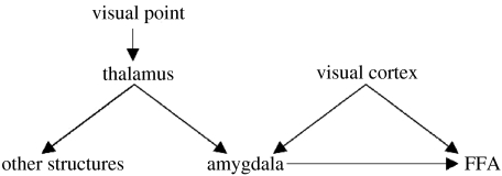
A neural system is an instance of a complex network. A convenient representation is that of a graph (figure 1) defined by a set of nodes that represents observed or unobserved (latent) variables, a set of edges, that indicate relations between nodes, and a set of probability statements about these relations (Speed & Kiiveri 1986; Wermuth & Lauritzen 1990; Cowell et al. 1999; Jensen 2002; Jordan 2004). Graphs, with only undirected edges, have been extensively used in the analysis of covariance relations (Wermuth & Lauritzen 1990; Wermuth & Cox 1998, 2004), but do not attempt causal interpretations. Neuroimaging studies based on this type of model will identify what Friston has defined as ‘functional connectivity’ (Friston 1994). To apply graphical models to functional neuroimaging data, one must be aware of the additional specificity that they are vector-valued time-series, with the vector of observations at time t, observed at Nt time instants. The p components of the vector are sampled at different nodes or spatial points in the brain. There has been much recent work in combining graphical models with multiple time-series analysis. An excellent example of the use of undirected graphs in the frequency domain is Bach & Jordan (2004) with applications to fMRI functional connectivity in Salvador et al. (2005).
Figure 1.
Directed graphical model of a (hypothetical) brain-causal network. Each node in the graph denotes a brain structure. An arrow between two nodes indicates that one structure (parent) exerts a causal influence on another node (child), a relation also known as ‘effective connectivity’. For functional images (EEG or fMRI), observations at each node are time-series. It should be noted that, optimally, time-series from all brain regions should be analysed simultaneously. Ignoring, for example, the amygdala might lead to erroneous conclusions about the influence of visual cortex on FFA, if only the latter were observed. A necessary (but not sufficient) condition for effective connectivity is that knowledge of activity in the parent improves prediction in the child (Granger causality). It is assumed that the set of directed links in real networks is sparse and therefore can be recovered by regression techniques that enforce this property.
A different line of work is represented by Pearl (1998, 2000, 2003) and Spirtes et al. (1991, 1998, 2000), among others, who studied graphs with directed edges that represent causal relations between variables. In the context of neuroimaging, searching for causality is what Friston terms the identification of effective connectivity. We will be concerned with this more ambitious type of modelling.
For functional neuroimages, the arrow of time may be used to help in the identification of causal relations. To be more specific, we model these time-series by means of a linear (stationary) multivariate autoregressive (MAR) model (Hamilton 1994; Harrison et al. 2003). While this type of model is very restrictive and brain-unrealistic, it will serve our purpose of developing methods for identifying connectivities in large complex neural networks for which the number of nodes p is very large compared with Nt. The general MAR model reads:
| (1.1) |
The dynamics of the process modelled are determined by the matrices of autoregressive coefficients that are defined for different time lags k and the spatial covariance matrix of , the white-noise input process (innovations). MAR modelling has been widely applied in neuroscience research (Baccala & Sameshima 2001; Kaminski et al. 2001; Harrison et al. 2003).
Note that the coefficients measure the influence that node j exerts on node i after k time instants. Knowing that is non-zero is equivalent to establishing effective connectivity and is also closely related to the concept of Granger causality (Granger 1969; Kaminski et al. 2001; Goebel et al. 2003; Hesse et al. 2003; Valdes-Sosa 2004; Eichler 2005). The merge of causality analysis (Pearl 1998, 2000; Spirtes et al. 1991, 2000) with multi-time-series theory has originated graphical time-series modelling as exemplified in Brillinger et al. (1976); Dahlhaus (1997); Dahlhaus et al. (1997); Eichler (2004; 2005).
Unfortunately there is a problem with this approach when dealing with neuroimaging data: the brain is a network with extremely large p, in the order of hundreds of thousands. A ‘curse of complexity’ immediately arises. The total number of parameters to be estimated for model (1.1) is , a situation for which usual time-series methods break down. One approach to overcome this curse of complexity is to pre-select a small set of regions of interest (ROI), on the basis of prior knowledge. Statistical dependencies may then be assayed by standard methods of time-series modelling (Hamilton 1994) that in turn are specializations of multivariate regression analysis (Mardia et al. 1979). The real danger is the probable effect of spurious correlations induced by the other brain structures not included for study. Thus, the ideal would be to develop MAR models capable of dealing with large p.
An alternative to using ordinary multivariate regression techniques for model (1.1) is to attempt regression based on selection of variables. This could drastically reduce the number of edges in the network graph to be determined, effectively restricting our attention to networks with sparse connectivity. That this is a reasonable assumption is justified by studies of the numerical characteristics of network connectivity in anatomical brain databases (Sporns et al. 2000; Stephan et al. 2000; Hilgetag et al. 2002; Kotter & Stephan 2003; Sporns et al. 2004). The main objective of this paper is to develop methods for the identification of sparse connectivity patterns in neural systems. We expect this method to be scaled, eventually, to cope with hundreds or thousands of voxels. Explicitly, we propose to fit the model with sparsity constraints on and .
Researchers into causality (Scheines et al. 1998; Pearl 2000) have explored the use of regression by the oldest of variable selection techniques—stepwise selection for the identification of causal graphs. This is the basis of popular algorithms such as principal components embodied in programmes such as Tetrad. These techniques have been proposed for use in graphical time-series models by Demiralp & Hoover (2003). Unfortunately these techniques do not work well for large p/Nt ratios. A considerable improvement may be achieved by stochastic search variable selection (SSVS), which relies on Markov chain–Monte Carlo (MCMC) exploration of possible sparse networks (Dobra et al. 2004; Jones & West 2005). These approaches, however, are computationally very intensive and not practical for implementing a pipeline for neuroimage analysis.
A different approach has arisen in the data mining context, motivated to a great extent by the demands posed by analysis of micro-array data (West 2002; Efron et al. 2004; Hastie & Tibshirani 2004; Hastie et al. 2001). This involves extensive use of Bayesian regression modelling and variable selection, capable of dealing with the p≫Nt situation. Of particular interest is recent work in the use of penalized regression methods for existing variable selection (Fan & Li 2001; Fan & Peng 2004) which unify nearly all variable selection techniques into an easy-to-implement iterative application of minimum norm or ridge regression. These techniques have been shown to be useful for the identification of the topology of huge networks (Leng et al. 2004; Meinshausen & Bühlmann 2004).
Methods for variable selection may also be combined with procedures for the control of the false discovery rates (FDR) (Efron 2003, 2004, 2005) in situations where a large number of null hypothesis is expected to be true. Large p in this case becomes a strength instead of a weakness, because it allows the non-parametric estimation of the distribution of the null hypotheses to control false discoveries effectively.
In a previous paper, Valdes-Sosa (2004) introduced a Bayesian variant of MAR modelling that was designed for the situation in which the number of nodes far outnumbers the time instants (p≫Nt). This approach is, therefore, useful for the study of functional neuroimaging data. However, that paper stopped short of proposing practical methods for variable selection. The present work introduces a combination of penalized regression with local FDR methods that are shown to achieve efficient detection of connections in simulated neural networks. The method is additionally shown to give plausible results with real fMRI data and is capable of being scaled to analyse large datasets.
It should be emphasized that in the context of functional imaging there are a number of techniques for estimating the effective connectivity, or edges, among the nodes of small pre-specified neuroanatomic graphs. These range from maximum likelihood techniques using linear and static models (e.g. structural equation modelling; McIntosh & Gonzalez-Lima 1994) to Bayesian inference on dynamic nonlinear graphical models (e.g. dynamic causal modelling; Friston et al. 2003). Almost universally, these approaches require the specification of a small number of nodes and, in some instances, a pre-specified sparsity structure, i.e. elimination of edges to denote conditional independence among some nodes. The contribution of this work is to enable the characterization of graphical models with hundreds of nodes using the short imaging time-series. Furthermore, the sparsity or conditional independence does not need to be specified a priori but is disclosed automatically by an iterative process. In short, we use the fact that the brain is sparsely connected as part of the solution, as opposed to treating it as a specification problem.
The structure of this paper is as follows. The subsequent section introduces a family of penalized regression techniques useful for identifying sparse effective connectivity patterns. The effectiveness of these methods for detecting the topology of large complex networks is explored in §2 by means of extensive simulations and is quantified by means of ROC measures. These methods are then applied together with local FDR techniques to evaluate real fMRI data. The paper concludes with a discussion of implications and possible extensions.
2. Sparse MAR models
We now describe a family of penalized regression models that will allow us to estimate sparse multivariate autoregressive (SMAR) models. In the following we shall limit our presentation to first order SMAR models in which Nk=1. This will simplify the description of models and methods, allowing us to concentrate on conceptual issues. Previous studies (Martinez-Montes et al. 2004; Valdes-Sosa 2004) have shown that first order MAR models fit fMRI data well (as indicated by the model selection criteria such as GCV, AIC or BIC). However, it is clear that for other types of data such as EEG, more complex models are necessary. All expressions given below generalize to the more complete model. In fact, all software developed to implement the methods described has been designed to accommodate all model orders.
We first review classical MAR methods. For a first order MAR equation (1.1) simplifies to:
| (2.1) |
where et is assumed to follow a multivariate Gaussian distribution N(0, Σ), with zero mean 0(p×1) and precision matrix .
This model can be recast as a multivariate regression:
| (2.2) |
where we define and introduce the notation:
Usual time-series methods rely on maximum likelihood (ML) estimation of model (2.2), which is equivalent to finding:
| (2.3) |
This has an explicit solution, the OLS estimator:
| (2.4) |
It should be noted that the unrestricted ML estimator of the regression coefficients does not depend on the spatial covariance matrix of the innovations (Hamilton 1994). One can therefore carry out separate regression analyses for each node. In other words, it is possible to estimate separately each column βi of B:
| (2.5) |
where zi is the i-th column of Z. It is to be emphasized that these definitions will work only if m≫p. Additionally, it is also well known that OLS does not ensure sparse connectivity patterns for A1. We must therefore turn to regression methods specifically designed to ensure sparsity.
The first solution that comes to mind is to use the readily available stepwise variable selection methods. Such is the philosophy of Tetrad (Glymour et al. 1988; Spirtes et al. 1990). Unfortunately, stepwise methods are not consistent (Hastie et al. 2001). This means that even increasing the sample size indefinitely (Nt→∞) does not guarantee the selection of the correct set of non-zero coefficients. This result still holds even if all subsets of variables are exhaustively explored.
Procedures with better performance are those based on Bayesian methods in which assumptions about B are combined with the likelihood by means of Bayes’ theorem. A very popular method is stochastic search variable selection (SSVS) (George & McCulloch 1997; George 2000). SSVS is based on a hierarchical model in which the first stage is just the likelihood defined by equation (2.1), and the other stage assumes that the elements of B (β) are each sampled a priori from a mixture of two probability densities: . The density is concentrated around zero, while has a larger variance. The decision of sampling from either is taken with binomial probabilities p0 and (1−p0), respectively. When p0 is large, this means we expect the matrix B to be very sparse. The model is explored using Monte Carlo–Markov chain techniques. This limits the application of this method to a rather small number of nodes p as analysed in Dobra et al. (2004), Dobra & West (2005) and Jones et al. (2005).
For this reason, we chose to explore other methods as alternatives to SSVS for variable selection, giving preference to those that were computationally more feasible. There has been much recent attention on different forms of penalized regression models. The simplest and best known of this family of methods is ridge regression (Hoerl & Kennard 1970), also known as quadratic regularization, which substitutes the argument (2.3) for the following one:
| (2.6) |
Minimization of this functional leads to the estimator:
| (2.7) |
λ being the regularization parameter which determines the amount of penalization enforced. There are very efficient algorithms based on the singular value decomposition for calculating these estimators as well as their standard errors. Forms of ridge regression have been recently applied (with P=Ip) to analyse micro-array data by West (2002) and (with P a spatial Laplacian operator) to study fMRI time-series by Valdes-Sosa (2004). These papers showed the ability of this method to achieve stable and plausible estimates in the situation p≫n. In the present paper, we explore the feasibility of using ridge regression as part of a technique for variable selection. It should be clear that ridge regression does not carry out variable selection per se. For this reason it is necessary to supplement this procedure with a method for deciding which coefficients of are actually zero. This will be described in detail below.
Following ridge regression, a number of penalized regression techniques have been introduced in order to stabilize regressions and perform variable selection. All these methods can be expressed as the solution of the minimization of:
| (2.8) |
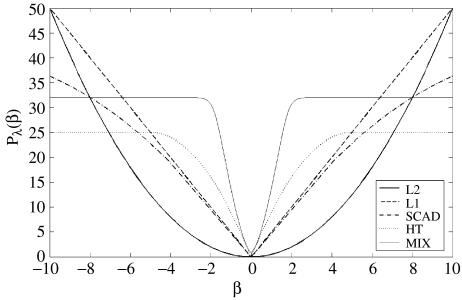
where is the penalty function applied to each component of the vector of regression coefficients β. The form of different penalty functions as a function of the current value of a regression coefficient β is shown in figure 2. It should be noted that the quadratic function is the ridge regression described above. Another type of penalty, perhaps one of the best known in the statistical learning literature, is the LASSO (Hastie et al. 2001), or L1 norm. This method has been recently implemented with great computational efficiency (Efron et al. 2004).
Figure 2.
Penalization functions used for the iterative estimation of sparse causal relations. At each step of the iterative process, the regression coefficients of each node with all others are weighted according to their current size. Many coefficients are successively down-weighted and ultimately set to zero—effectively carrying out variable selection. y-Axis: weight according to current value of a regression coefficient β (x-axis). Each curve corresponds to a different type of penalization: heavy line, L2 norm (ridge regression); dashed, L1 norm (LASSO). Dotted, Hard-Threshold; dash-dot, SCAD; light line, mixture.
During the process of implementing algorithms for each type of penalty function, advantage was taken of the recent demonstration by Fan & Li (2001), Fan & Peng (2004), Hunter (2004) and Hunter & Lange (2004) that estimation of any one of many penalized regressions can be carried out by iterative application of ridge regression:
| (2.9) |
where , a diagonal matrix is defined by and is the derivative of the penalty function being evaluated.
The algorithm described by Fan & Peng (2004) unifies a large number of penalized regression techniques. These are summarized in table 1, in which the derivatives of the penalty functions are provided.
Table 1.
Derivatives of penalty functions.
| type of penalization | derivative |
|---|---|
| LASSO | |
| SCAD | |
| Hard-Threshold | |
| ridge | |
| MIX | |
| Γ(·) denotes the Gamma function |
The reason that this algorithm works may be inferred from figure 2. At each step of the iterative process, the regression coefficients of each node with all others are weighted according to their current size. Many coefficients are successively down-weighted and ultimately set to zero—effectively carrying out variable selection in the case of the LASSO, Hard-Threshold and SCAD penalization. It must be emphasized that the number of variables set to zero in any of the methods described will depend on the value of the regularization parameter λ with higher values selecting fewer variables. In this paper, the value of the tuning parameter λ was selected to minimize the generalized crossvalidation criterion (GCV).
The penalizations explored in this article for variable selection are:
ridge: the L2 norm;
LASSO: the L1 norm;
Hard-Thresholding;
SCAD: smoothly clipped absolute deviation penalty of Fan & Li (2001); and
MIX: mixture penalty.
It came as a pleasant surprise to us during the programming of the variable selection algorithms, that the SSVS of George & McCulloch (1997) can also be expressed as a penalized regression with penalty . We therefore added to the comparisons this ‘quick and dirty’ implementation of SSVS as the MIX criteria which also carries out automatic variable selection.
The specific implementation of penalized regression used in this article is that of the maximization–minorization (MM) algorithm (Hunter 2004; Hunter & Lange 2004), which exploits an optimization technique that extends the central idea of EM algorithms to situations not necessarily involving missing data, nor even ML estimation. This new algorithm retains virtues of the Newton–Raphson algorithm. All algorithms were implemented in Matlab 7.0 and will be made available on the website of this journal.
Additionally, the iterative estimation algorithm allows us to compute the covariance matrix of the resulting regression coefficient via a ‘sandwich formula’. This allows the estimation of standard errors for different contrasts of interest. For example, these standard errors were used to define a t statistic for each autoregressive coefficient to test its presence, or to calculate confidence intervals for different contrasts.
3. Performance of penalized regression methods with simulated data
(a) Description of simulations
In order to measure the performance of different penalized regression methods for estimating SMAR models, a number of simulations were carried out. For this purpose, a universe of idealized cortical models was defined based on the concept of ‘small world topology’ (Watts & Strogatz 1998; Albert & Barabasi 2002; Jirsa 2004; Sporns et al. 2004; Sporns & Zwi 2004; Sporns 2005).
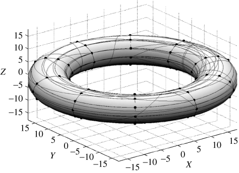
The simulated ‘cortex’ was defined as a set of nodes comprising a two-dimensional grid on the surface of a torus (figure 3). This geometry was chosen to avoid special boundary conditions since the network is periodic in the plane in both dimensions. For each simulation a set of directed connections was formed randomly. Following Sporns & Zwi (2004), the existence of a directed connection between any nodes i and j was sampled from a binomial distribution with probabilities pij. These probabilities were in turn sampled from a mixture density:
The Gaussian component of the mixture (depending on distance) will produce short-range connections and induce high clustering among nodes. The uniform component of the mixture ensures the presence of long-range connections which induce short-path lengths between any pair of nodes in the network. The parameters of the mixture (α, γ) were tuned by hand to produce a ‘small world’ effect, which was in practice, possible with only a small proportion of uniformly distributed connections. The directed links for one sample network are shown on the surface of the torus in figure 3.
Figure 3.
Idealized cortical models used to test regression methods for the identification of sparse graphs were simulated by a ‘small world’ network topology. Nodes resided on a two-dimensional grid on the surface of a torus, thus imposing periodic boundary conditions in the plane. For each simulation, a set of directed connections was first formed with a distribution crafted to induce the ‘small world effect’. The strengths of the connections between parents and children were sampled from a Gaussian distribution. Directed links are shown on the surface of the torus for one sample network.
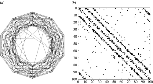
A more detailed view of a sample small-world network is shown in figure 4 which shows in (a) the two-dimensional view of the links between nodes and in (b), their connectivity matrix. Once the connectivity matrix of the network was defined, the strengths of the connections between parents and children were sampled from a Gaussian distribution truncated around zero with a variable threshold τ. With higher τ, only stronger connections were allowed, thus increasing the ‘signal to noise ratio’ for the detection of network connections. The resulting matrix of (auto)regressive coefficients A1 of the network has the same sparsity structure as that of the connectivity matrix. Those A1 with singular values greater than one were rejected from the simulation, since our purpose was to study stable SMAR models.
Figure 4.
Connectivity structure of the simulated cortical network shown in figure 3. This type of small-world network has a high probability of connections between geographical neighbours and a small proportion of larger range connections. The network mean connectivity was: 6.23; the scaled clustering: 0.87; the scaled length: 0.19. (a) Two-dimensional view of the links between nodes. (b) Connectivity (0–1) matrix in with a row for each node and non-zero elements for its children.
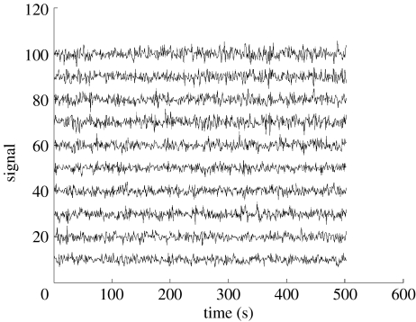
Simulated fMRI time-series were generated by the first order SMAR model (2.1) with the connectivity matrix obtained as described above. A random starting state was selected, and then a ‘burning in’ period of several thousand samples was first generated and discarded to avoid system transients. Subsequent samples were retained for the analyses presented below. The result of this process, a typical fMRI simulation is shown in figure 5.
Figure 5.
Simulated fMRI time-series generated by a first order multivariate autoregressive model , the autoregressive matrix being sampled as described in figures 3 and 4. The innovations et (noise input) were sampled from a Gaussian distribution with a prescribed inverse covariance matrix Σ-1 as described in figure 6. Y-axis: simulated BOLD signal, x-axis: time. The effect of different observed lengths of time-series (N) on the detection of connections was studied.
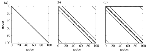
Simulations with different types of innovations et were carried out. They differed in the type of inverse covariance matrices from which they were generated. Three variants of connectivity patterns for the spatial covariance Σ of the innovations were used to simulate fMRI time-series. Shown in figure 6 are the connectivity matrices for the precisions Σ−1 (a) spatial independence with a diagonal precision matrix, (b) nearest-neighbour dependency with partial autocorrelations existing only between nodes close to each other, (c) nearest-neighbour topology with an additional ‘master’ node linked to all other nodes in the network.
Figure 6.
Connectivity matrices for the precisions Σ−1. Three situations were explored: (a) spatial independence with a diagonal precision matrix, (b) nearest-neighbour dependency with partial autocorrelations existing only between nodes close to each other, (c) nearest-neighbour topology with a ‘master’ node linked to all other nodes in the network.
(b) Comparison of methods
It must be remembered that the purpose of the simulations was to generate time-series from which the network topology of the idealized cortical network could be estimated. As is usual in the evaluation of diagnostic methods, a number of indices were calculated to evaluate the performance of different penalized regression techniques. For reference purposes, the definition of these indices is summarized in table 2.
Table 2.
Definition of quantities used for assessing the methods network reconstruction.
| quantity | definition |
|---|---|
| number of true edges | TP+FN |
| number of zero-edges | TN+FP |
| significant edges | TP+FP |
| detection rate | TP/(TP+FN) |
| false alarm rate | FP/(TN+FP) |
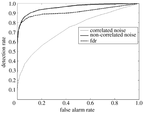
The actual sensitivity and specificity of each regression method depends, of course, on the threshold selected to reject the null hypothesis for the t statistic of each regression coefficient. Overall performance for each regression method under different conditions was measured by means of their receiver operating characteristic (ROC) curves which are, as is well known, the representation of the tradeoffs between sensitivity (Sn) and specificity (Sp) (table 2). The plot shows false alarm rate (1−Sp) on the x-axis and detection rate (Sn) on the y-axis. ROC curves are further summarized by their areas, which we shall call for brevity the ‘detection efficiency’. In all comparisons, at least 25 simulated fMRI series were generated. For each comparison, each method was represented by its worst case scenario, the ROC curve with the lowest detection efficiency for all 25 replications. A typical example of ROC curves is shown in figure 7, which corresponds to ridge regression applied to a simulated network with p=100 nodes and a recorded length of Nt=200 time points. The dark line corresponds to a simulated fMRI generated with spatially independent noise, as well as with a high signal to noise ratio. The ROC curve is well above the diagonal line that would be the result with a random detection procedure.
Figure 7.
Efficiency of ridge regression for the detection of causal connections in simulated fMRI from a network with p=100 nodes and a recorded length of Nt=200 time points, as measured by receiver operating curves (ROC). y-Axis: probability of detection of true connections, x-axis: probability of false detections. The dark line corresponds to an fMRI generated with spatially independent noise as well as with a high signal to noise ratio. The thin line corresponds to a time-series generated with spatially correlated noise (nearest neighbour), as well as with a low signal to noise ratio. Note the decreases of detection efficiency with these factors. The dashed line shows the performance of the local false discovery rate thresholds calculated without knowledge of the true topology of the network. Note the excellent correspondence at low false-positive rates.
From the whole set of simulations a number of findings can be summarized.
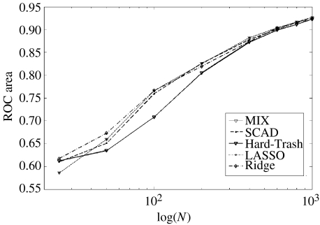
In the first place, the detection efficiency in all simulations was well above the chance level, validating the hypothesis that penalized regression techniques are useful for the detection of connectivity topologies in complex networks. The difference between penalization techniques was rather disappointing, as summarized in figure 8 which shows that all methods are roughly equivalent with respect to detection efficiency. Exceptions are the hard threshold penalty which performs slightly worse than the others and ridge regression that performs slightly better. In view of the ease with which ridge regression is computed, there seems to be no point in using more complicated techniques. For this reason, from now onwards, unless explicitly stated, all results presented and discussed correspond to ridge regression.
Figure 8.
Effect of the ratio of network size (p) to temporal sample size (Nt) on the detection efficiency for different penalized regression methods. The number of nodes in the network was kept at p=100. y-Axis: area under ROC curve. x-Axis: sample size (N). Though efficiency decreases with smaller sample sizes, all methods perform well above chance even for p=4N. Ridge regression dominates the other methods for p=N with no significant differences at other p/Nt ratios
With regard to the p/Nt ratio, figure 8 shows the detection efficiency as a function of Nt for a fixed number of nodes ( p=100). All methods perform equally well when the number of nodes is small with regard to the number of time points. Efficiencies decrease uniformly when the number of data points decreases but are well above chance levels even for p=4Nt.
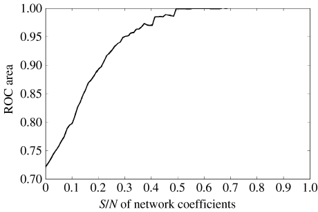
Detection efficiency depends monotonically on the S/N ratio connection strength. Figure 9 shows that even with networks with small connection strengths relative to the system noise, good detection efficiencies are possible (LASSO penalization).
Figure 9.
Effect of signal to noise ratio of network connectivity generation on efficiency of detection by LASSO. y-Axis: area under the ROC, x-axis: signal to noise ratio.
Strong spatial correlations in the innovations tended to diminish the detection efficiency for A1 with respect to the uncorrelated case. The worse performance is with innovations generated from precision matrices with strong structure and a master driving node. The thin line in figure 7 corresponds to a time-series generated with both spatially correlated innovations (nearest-neighbour topology), as well as with a low signal to noise ratio. Note the interaction of both factors that produce marked decreases of detection efficiency when compared with the situation denoted by the thick line (high S/N and no spatial correlation).
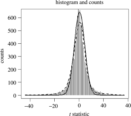
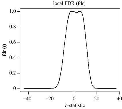
For the real fMRI experiments, we must select a threshold for rejecting the null hypothesis. This involves multiple comparisons for a large number of autoregressive coefficients. The simulations gave us the opportunity of checking the usefulness for this purpose of the FDR procedure introduced by Benjamini & Hochberg (1995). Given a set of p hypotheses, out of which an unknown number p0 are true, the FDR method identifies the hypotheses to be rejected, while keeping the expected value of the ratio of the number of false rejections to the total number of rejections below q, a user-specified control value. In the present paper we use a modification of this procedure, the ‘local’ FDR (which we shall denote as ‘fdr’ in lower case) as developed by Efron (2003, 2004, 2005). Multiple tests are modelled as being sampled from the mixture of two densities given by , which are estimated with non-parametric methods. An R program Locfdr is available from the CRAN website for this calculation. The fdr procedure was used to analyse the same data used to generate figure 7. Figure 10 shows the results of applying locfdr which estimates the t statistics for all regression coefficients as the mixture of two of the null and alternative densities. Figure 11 shows the fdr curve produced which allows the selection of a threshold with a given local false-positive rate. Looking back to figure 7, the dashed line shows the performance of the local fdr thresholds calculated without knowledge of the true topology of the network. Note the excellent correspondence between the fdr and the ROC curve at low false-positive rates.
Figure 10.
The local FDR (fdr) is ideal for the detection of sparse connections. If there are few connections, then testing for links between all nodes should lead to a sample of test statistics for which the null hypothesis predominates. The distribution of the statistics can therefore be modelled as a mixture of the density of null hypothesis with that of the alternative hypothesis. These are separated by non-parametric density estimation as shown in this figure, in which the thick line denotes the estimated null distribution and the thin one the estimated alternative distribution for the ridge regression example shown in figure 7 (thick line). y-Axis: counts, x-axis: values of the t statistics for estimated regression coefficients.
Figure 11.
The local false discovery of the ridge regression example of figure 7. y-Axis: fdr, x-axis: t statistic for estimated regression coefficients.
4. Analysis of fMRI data
A combination of ridge regression and local FDR was used to analyse fMRI data recorded during a face processing experiment. No attempt was made to reach exhaustive substantive conclusions about the experiment analysed, since the purpose of this exercise was only to demonstrate the feasibility of working with the new methods. The experimental paradigm consisted of the presentation of faces of both men and women under the following conditions:
Condition 1: static faces with fearful expressions (SFF);
Condition 2: neutral faces (with no emotional content), (NF);
Condition 3: dynamic fear faces (in this condition faces are morphed from neutral emotional content to fear; DFF).
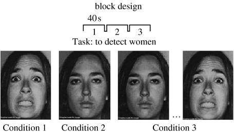
The subject was asked to count the number of faces that belonged to women. Stimuli were presented in a block design with the following order: SFF—NF—DFF. Each block lasted 40 s and was repeated six times. The experiment duration was 720 s=12 min. The duration of each stimulus was 1 s for each condition. Stimuli presentation and synchronization to the MR scanner was performed using Cogent modelling software v.2.3 (http://cogent.psyc.bbk.ac.uk/; figure 12).
Figure 12.
fMRI acquisition: the experimental paradigm consisted of visual stimuli presented under three conditions. Condition 1, static fearful faces, (SFF); Condition 2, neutral faces (with no emotional content), (NF); Condition 3, dynamic fearful faces (in this condition faces are morphed from neutral emotional content to fear; DFF). A general linear model was posited that included not only a different mean level μC vector, but also a different autoregressive matrix for each condition C. Thus, the model explores changes across voxels not only of mean level of activity but also of connectivity patterns.
Images were acquired using a 1.5 T Symphony Scanner, Siemens, Erlangen, Germany. Functional images were acquired using a T2* weighted echo planar sequence in 25 oblique slices (interleave acquisition). The EPI sequence was defined by: TE=60 ms, TR=4000 ms, flip angle: 90 °, FOV=224 mm, slice thickness: 3.5 mm, acquisition matrix=64×64. The number of scans recorded was 185. The first five scans were rejected for the analysis because of T1 saturation effect. A high resolution anatomical image acquisition was also acquired using a T1 MPRAGE sequence (TE=3.93 ms/TR=3000 ms), voxel size=1×1×1 mm3, FOV=256 mm. Matrix size=256×256.
The fMRI data were first analysed using the Statistical Parametric Mapping Software package SPM2 (www.fil.ion.ucl.ac.uk/spm/software/spm2/). Preprocessing with SPM was restricted to the following steps: (i) slice time correction (using trilinear interpolation); (ii) motion correction; (iii) unwarping. No temporal smoothing was used. As a preliminary check, using standard SPM procedures for the comparison of conditions it was possible to show activation of fusiform face area (FFA) as well as involvement of limbic structures to the presentation of fearful faces.
Inspection of the fMRI time-series for all fMRI voxels revealed a rhythmic artefact, synchronous for all voxels that was eliminated by suppression of the first pair of singular vectors in the SVD decomposition of the raw data matrix. In order to reduce the spatial dimensions of the data, the subject's MRI time was segmented into 116 different structures using an automated procedure and based on the macroscopic anatomical parcellation of the MNI MRI single-subject brain used by Tzourio-Mazoyer et al. (2002). The fMRI time-series data were spatially averaged over these ROI to yield 116 time-series.
For the analysis of these data, model (2.1) was expanded to:
| (4.1) |
where dt is a drift term estimated by a second-order polynomial defined over the whole experiment, μC is the mean level for conditions and the condition-dependent autoregressive matrices. Thus, the model explores changes across voxels, not only of mean level of activity, but also of connectivity patterns. We decided to compare conditions SFF and DFF (fearful faces). The model was fitted by means of ridge regression (with no regularization on the drift and condition mean effects). t Statistics were computed for the relevant contrasts.
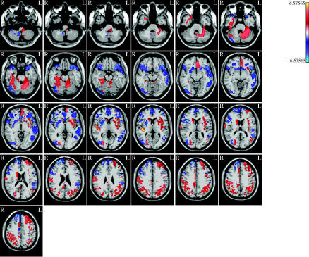
Figure 13 shows the tomography of the t statistics contrasting the average of the fearful face means with that of neutral faces . The map is thresholded using the local FDR (fdr) as explained above with q=0.01. Note the activation of the FFA area which was very similar to that obtained with the analysis carried out with SPM2.
Figure 13.
Tomography of t statistics contrasting fearful face means with that of neutral faces μNF. t-Values are obtained by Bayesian ridge regression and thresholded using the local FDR (fdr) as explained in figures 10 and 11. Note the activation of the FFA which was very similar to that obtained with the SPM package.
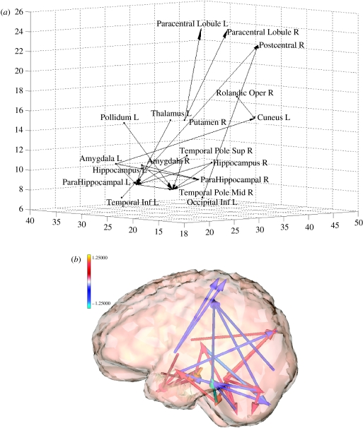
A similar analysis was carried out with the connectivity matrices (figure 14). The contrast compared the pooled estimate of fearful faces to that of neutral faces (). Graphs are constructed with only those edges which fell above the fdr threshold for the t statistics of the contrast. Both (a) and (b) of figure 14 show the same data with a more schematic and a more realistic rendering, respectively. It is interesting to note the involvement of brain structures involved in processing emotional stimuli. Absent are connections to FFA which have approximately the same level in all face conditions.
Figure 14.
(a) Graph of connections that change with appearance of fearful expression. Obtained by element wise comparison of the autoregressive matrices of fearful faces as compared with that of neutral faces (). Only those connections above the fdr threshold are shown. Note involvement of areas related to emotional responses. (b) Three-dimensional rendering of the connectivity patterns shown in (a).
5. Discussion
This paper proposes a method for identifying large scale functional connectivity patterns from relatively short time-series of functional neuroimages. The method is based on estimating SMAR models by a two-stage process that first applies penalized regression (Fan & Peng 2004), and is then supplemented by pruning of unlikely connections by use of the local FDR procedure developed by Efron (2003). The methods are demonstrated to perform well in identifying complex patterns of network connectivity by means of simulations on an idealized small world cortical network. These simulations also show that the simplest of the methods, ridge regression, performs as well as more sophisticated and recent techniques. This does not rule out that the performance of other penalized techniques might be improved, for example, by a better estimate of the regularization parameter, just to mention one possibility. Of particular interest is the complete exploration, not carried out in the present project owing to time constraints, of the mixture penalties that provide a bridge between SSVS (George & McCulloch 1997) and penalized regression techniques.
The simulations also highlight an important area for improvement. The detection efficiency of penalized regression decreases with unobserved correlations between the inputs of the system which in graphical models correspond to unobserved latent variables. This is in agreement with theoretical insights provided by statistical analyses of causality (Pearl 1998), as well as being part of the accumulated experience of time-series analysis in the neurosciences (Kaminski et al. 2001). Part of the problem is the relative unreliability of estimating very large dimensional covariance matrices. Inspection of table 3 shows that estimation and use of the covariance matrix of the innovations does not improve the detection efficiency for autoregressive coefficients.
Table 3.
Effect on detection efficiency of different spatial correlation patterns of the innovations for a network with p=100 and Nt=60.
| Σ−1 | detection efficiency for A1 estimated alone | detection efficiency for A1 estimated with information about Σ−1 |
|---|---|---|
| diagonal | 0.8001 | 0.8012 |
| nearest neighbour | 0.7873 | 0.7880 |
| nearest neighbour with master node | 0.6747 | 0.6298 |
The two columns correspond to the detection efficiencies for estimates that do not take into consideration Σ−1 and those that do.
The assumption of sparsity of neural connections has been supported by quantitative studies of databases of neural connections (Hilgetag et al. 2002). Sparseness is a central concept of modern statistical learning (Gribonval et al. 2005), but had not been applied, to our knowledge, to the estimation of MAR models. This general requirement for sparsity may be combined in the future with the information provided by fibre tractography methods based on diffusion MRI.
The simulations presented and the real fMRI example analysed comprised 100 and 116 time-series, respectively. Although falling short of the spatial dimensionality of functional neuroimages, they represent an order of magnitude increase in the size of problem than those that are solvable standard time-series techniques. The methods and software developed have been tested to be scalable for the analysis of hundreds of thousands of voxels.
For the sake of simplicity, the SMAR has been posited to be linear, stationary and to involve only lags of the first order. It is relatively straightforward to generalize this formalism to the analysis of more complex situations. Such extensions have already been carried out for the small p case for non-stationary time-series analysis (Hesse et al. 2003) and for nonlinear processes (Freiwald et al. 1999). Work is currently in progress to apply sparse restrictions in order to address more realistic assumptions when modelling functional neuroimages.
While it is true that nothing can substitute for the lack of data, the next best thing, if the data are scarce, is not to use it in estimating things that are probably not there.
Acknowledgments
The authors thank Mitchell Valdés-Sosa, Maria A. Bobes-León, Nelson Trujillo Barreto and Lorna García-Pentón for providing the experimental data analysed in this paper, as well as for valuable insights and support.
Footnotes
One contribution of 21 to a Theme Issue ‘Multimodal neuroimaging of brain connectivity’.
References
- Albert R, Barabasi A.L. Statistical mechanics of complex networks. Rev. Modern Phys. 2002;74:47–97. [Google Scholar]
- Baccala L.A, Sameshima K. Partial directed coherence: a new concept in neural structure determination. Biol. Cybern. 2001;84:463–474. doi: 10.1007/PL00007990. [DOI] [PubMed] [Google Scholar]
- Bach F.R, Jordan M.I. Learning graphical models for stationary time series. IEEE Trans. Signal Proc. 2004;52:2189–2199. [Google Scholar]
- Benjamini Y, Hochberg Y. Controlling the false discovery rate—a practical and powerful approach to multiple testing. J. R. Stat. Soc. B Methodological. 1995;57:289–300. [Google Scholar]
- Brillinger D.R, Bryant H.L, Segundo J.P. Identification of synaptic interactions. Biol. Cybern. 1976;22:213–228. doi: 10.1007/BF00365087. [DOI] [PubMed] [Google Scholar]
- Bullmore E, Harrison L, Lee L, Mechelli A, Friston K. Brain connectivity workshop, Cambridge UK, May 2003. Neuroinformatics. 2004;2:123–125. [Google Scholar]
- Cowell R.G, Dawid P.A, Lauritzen S.L, Spiegelhalter D.J. Springer; New York: 1999. Probabilistic networks and expert systems. [Google Scholar]
- Dahlhaus R. Fitting time series models to nonstationary processes. Ann. Stat. 1997;25:1–37. [Google Scholar]
- Dahlhaus R, Eichler M, Sandkuhler J. Identification of synaptic connections in neural ensembles by graphical models. J. Neurosci. Methods. 1997;77:93–107. doi: 10.1016/s0165-0270(97)00100-3. [DOI] [PubMed] [Google Scholar]
- Demiralp S, Hoover K.D. Searching for the causal structure of a vector autoregression. Oxford Bull. Econ. Stat. 2003;65:745–767. [Google Scholar]
- Dobra, A. & West, M. 2005 HdBCS—Bayesian covariance selection. (See http://ftp.isds.duke.edu/WorkingPapers/04-23.pdf)
- Dobra A, Hans C, Jones B, Nevins J.R, Yao G.A, West M. Sparse graphical models for exploring gene expression data. J. Multivariate Anal. 2004;90:196–212. [Google Scholar]
- Efron B. Robbins, empirical Bayes and microarrays. Ann. Stat. 2003;31:366–378. [Google Scholar]
- Efron B. Large-scale simultaneous hypothesis testing: the choice of a null hypothesis. J. Am. Stat. Assoc. 2004;99:96–104. [Google Scholar]
- Efron, B. 2005 Bayesians, frequentists, and physicists. (See http://www-stat.stanford.edu/~brad/papers/physics.pdf)
- Efron B, Hastie T, Johnstone I, Tibshirani R. Least angle regression. Ann Stat. 2004;32:407–451. [Google Scholar]
- Eichler M. Brain Connectivity Workshop Havana, April 26–29. 2004. Causal inference with graphical time series models. p. 1. [Google Scholar]
- Eichler M. A graphical approach for evaluating effective connectivity in neural systems. Phil. Trans. R. Soc. B. 2005;360:953–967. doi: 10.1098/rstb.2005.1641. doi:10.1098/rstb.2005.1641 [DOI] [PMC free article] [PubMed] [Google Scholar]
- Fan J.Q, Li R.Z. Variable selection via nonconcave penalized likelihood and its oracle properties. J. Am. Stat. Assoc. 2001;96:1348–1360. [Google Scholar]
- Fan J.Q, Peng H. Nonconcave penalized likelihood with a diverging number of parameters. Ann. Stat. 2004;32:928–961. [Google Scholar]
- Freiwald W.A, Valdes P, Bosch J, Biscay R, Jimenez J.C, Rodriguez L.M, Rodriguez V, Kreiter A.K, Singer W. Testing non-linearity and directedness of interactions between neural groups in the macaque inferotemporal cortex. J. Neurosci. Methods. 1999;94:105–119. doi: 10.1016/s0165-0270(99)00129-6. [DOI] [PubMed] [Google Scholar]
- Friston K.J. Functional and effective connectivity in neuroimaging: a synthesis. Hum. Brain Mapp. 1994;2:56–78. [Google Scholar]
- Friston K.J, Harrison L, Penny W. Dynamic causal modeling. Neuroimage. 2003;19:1273–1302. doi: 10.1016/s1053-8119(03)00202-7. [DOI] [PubMed] [Google Scholar]
- George E.I. The variable selection problem. J. Am. Stat. Assoc. 2000;95:1304–1308. [Google Scholar]
- George E.I, McCulloch R.E. Approaches for Bayesian variable selection. Stat. Sinica. 1997;7:339–373. [Google Scholar]
- Glymour C, Scheines R, Spirtes P, Kelly K. Tetrad—discovering causal-structure. Multivariate Behav. Res. 1988;23:279–280. doi: 10.1207/s15327906mbr2302_13. [DOI] [PubMed] [Google Scholar]
- Goebel R, Roebroeck A, Kim D.S, Formisano E. Investigating directed cortical interactions in time-resolved fMRI data using vector autoregressive modeling and Granger causality mapping. Magn. Reson. Imaging. 2003;21:1251–1261. doi: 10.1016/j.mri.2003.08.026. [DOI] [PubMed] [Google Scholar]
- Granger C.W.J. Investigating causal relations by econometric models and cross-spectral methods. Econometrica. 1969;37:414. [Google Scholar]
- Gribonval R, Figueras i Ventura R.M, Vandergheynst P. A simple test to check the optimality of sparse signal approximations. 2005 (See http://lts1pc19.epfl.ch/repository/Gribonval2005_1167.pdf.) [Google Scholar]
- Hamilton J.D. Princeton University Press; Princeton, NJ: 1994. Time series analysis. [Google Scholar]
- Harrison L, Penny W.D, Friston K. Multivariate autoregressive modeling of fMRI time series. NeuroImage. 2003;19:1477–1491. doi: 10.1016/s1053-8119(03)00160-5. [DOI] [PubMed] [Google Scholar]
- Hastie T, Tibshirani R. Efficient quadratic regularization for expression arrays. Biostatistics. 2004;5:329–340. doi: 10.1093/biostatistics/5.3.329. [DOI] [PubMed] [Google Scholar]
- Hastie T, Tibshirani R, Friedman J. Springer; New York: 2001. The elements of statistical learning: data mining, inference, and prediction. [Google Scholar]
- Hesse W, Moller E, Arnold M, Schack B. The use of time-variant EEG Granger causality for inspecting directed interdependencies of neural assemblies. J. Neurosci. Methods. 2003;124:27–44. doi: 10.1016/s0165-0270(02)00366-7. [DOI] [PubMed] [Google Scholar]
- Hilgetag C, Kotter R, Stephan K.E. Computational methods for the analysis of brain connectivity. In: Ascoli G.A, editor. Computational neuroanatomy. Humana Press; Totowa, NJ: 2002. [Google Scholar]
- Hoerl A.E, Kennard W.R. Ridge regression—biased estimation for nonorthogonal problems. Technometrics. 1970;12:55. [Google Scholar]
- Horwitz B. The elusive concept of brain connectivity. NeuroImage. 2003;19:466–470. doi: 10.1016/s1053-8119(03)00112-5. [DOI] [PubMed] [Google Scholar]
- Hunter D.R. MM algorithms for generalized Bradley–Terry models. Ann. Stat. 2004;32:384–406. [Google Scholar]
- Hunter D.R, Lange K. A tutorial on MM algorithms. Am. Stat. 2004;58:30–37. [Google Scholar]
- Jensen F.R. Springer; New York: 2002. Bayesian networks and decision graphs. [Google Scholar]
- Jirsa V.K. Connectivity and dynamics of neural information processing. Neuroinformatics. 2004;2:183–204. doi: 10.1385/NI:2:2:183. [DOI] [PubMed] [Google Scholar]
- Jones, B., West, M. 2005 Covariance decomposition in undirected Gaussian graphical models. (See http://ftp.isds.duke.edu/WorkingPapers/04-15.pdf)
- Jones, B., Carvalho, C., Dobra, A., Hans, Ch. 2005 Experiments in stochastic computation for high-dimensional graphical models. Technical Report 2004-1(papers)
- Jordan M.I. Graphical models. Stat. Sci. 2004;19:140–155. [Google Scholar]
- Kaminski M, Ding M.Z, Truccolo W.A, Bressler S.L. Evaluating causal relations in neural systems: granger causality, directed transfer function and statistical assessment of significance. Biol. Cybern. 2001;85:145–157. doi: 10.1007/s004220000235. [DOI] [PubMed] [Google Scholar]
- Kotter R, Stephan M.E. Network participation indices: characterizing componet roles for information processing in neural networks. Neural Netw. 2003;16:1261–1275. doi: 10.1016/j.neunet.2003.06.002. [DOI] [PubMed] [Google Scholar]
- Lee L, Harrison L.M, Mechelli A. A report of the functional connectivity workshop, Dusseldorf 2002. NeuroImage. 2003;19:457–465. doi: 10.1016/s1053-8119(03)00062-4. [DOI] [PubMed] [Google Scholar]
- Leng C, Lin Y, Whaba G. A note on the Lasso and related procedures in model selection. 2004 (See http://www.stat.wisc.edu/~wahba/ftp1/tr1091rxx.pdf.) [Google Scholar]
- Mardia K.V, Kent J.T, Bibby J.M. Academic Press; London: 1979. Multivariate analysis. [Google Scholar]
- Martinez-Montes E, Valdés-Sosa P, Miwakeichi F, Goldman R, Cohen M. Concurrent EEG/fMRI analysis by multi-way partial least squares. NeuroImage. 2004;22:1023–1034. doi: 10.1016/j.neuroimage.2004.03.038. [DOI] [PubMed] [Google Scholar]
- McIntosh A.R, Gonzalez-Lima F. Structural equation modeling and its applications to network analysis in functional brain imaging. Hum. Brain Mapp. 1994;2:2–22. [Google Scholar]
- Meinshausen N, Bühlmann P. 2004. Consistent neighborhood selection for sparse high-dimensional graphs with the Lasso.http://stat.ethz.ch/research/research_reports/2004/123 [Google Scholar]
- Pearl J. Graphs, causality, and structural equation models. Sociol. Methods Res. 1998;27:226–284. [Google Scholar]
- Pearl J. Cambridge University Press; Cambridge: 2000. Causality. [Google Scholar]
- Pearl J. Statistics and causal inference: a review. Test. 2003;12:281–318. [Google Scholar]
- Salvador R, Suckling J, Schwarzbauer C, Bullmore E. Undirected graphs of frequency dependent functional connectivity in whole brain networks. Phil. Trans. R. Soc. B. 2005;360:937–946. doi: 10.1098/rstb.2005.1645. doi:10.1098/rstb.2005.1645 [DOI] [PMC free article] [PubMed] [Google Scholar]
- Scheines R, Spirtes P, Glymour C, Meek C, Richardson T. The TETRAD project: constraint based aids to causal model specification. Multivariate Behav. Res. 1998;33:65–117. doi: 10.1207/s15327906mbr3301_3. [DOI] [PubMed] [Google Scholar]
- Speed T.P, Kiiveri H.T. Gaussian markov distributions over finite graphs. Ann. Stat. 1986;14:138–150. [Google Scholar]
- Spirtes P, Scheines R, Glymour C. Simulation studies of the reliability of computer-aided model-specification using the tetrad-ii, eqs, and lisrel Programs. Sociol. Methods Res. 1990;19:3–66. [Google Scholar]
- Spirtes P, Glymour C, Scheines R. From probability to causality. Phil. Stud. 1991;64:1–36. [Google Scholar]
- Spirtes P, Richardson T, Meek C, Scheines R, Glymour C. Using path diagrams as a structural equation modeling tool. Sociol. Methods Res. 1998;27:182–225. [Google Scholar]
- Spirtes P, Glymour C, Scheines R. The MIT Press; Cambridge: 2000. Causation, prediction, and search. [Google Scholar]
- Sporns, O. 2005 Complex neural dynamics. (See http://www.indiana.edu/~cortex/cd2002_draft.pdf)
- Sporns O, Zwi J.D. The small world of the cerebral cortex. Neuroinformatics. 2004;2:145–162. doi: 10.1385/NI:2:2:145. [DOI] [PubMed] [Google Scholar]
- Sporns O, Toning G, Edelman G.M. Theoretical neuroanatomy: relating anatomical and functional connectivity in graphs and cortical connection matrices. Cereb. Cortex. 2000;10:127–141. doi: 10.1093/cercor/10.2.127. [DOI] [PubMed] [Google Scholar]
- Sporns O, Chialvo D.R, Kaiser M, Hilgetag C.C. Organization, development and function of complex brain networks. Trends Cogn. Sci. 2004;8:418–425. doi: 10.1016/j.tics.2004.07.008. [DOI] [PubMed] [Google Scholar]
- Stephan K.E, Hilgetag C.C, Burns G.A.P.C, O'Neill M.A, Young M.P, Kotter R. Computational analysis of functional connectivity between areas of primate cerebral cortex. Phil. Trans. R. Soc. B. 2000;355:111–126. doi: 10.1098/rstb.2000.0552. doi:10.1098/rstb.2000.0552 [DOI] [PMC free article] [PubMed] [Google Scholar]
- Tzourio-Mazoyer N, Landeau B, Papathanassiou D, Crivello F, Etard O, Delcroix N, Mazoyer B, Joliot M. Automated anatomical labeling of activations in SPM using a macroscopic anatomical parcellation of the MNI MRI single-subject brain. NeuroImage. 2002;15:273–289. doi: 10.1006/nimg.2001.0978. [DOI] [PubMed] [Google Scholar]
- Valdes-Sosa P.A. Spatio-temporal autoregressive models defined over brain manifolds. Neuroinformatics. 2004;2:239–250. doi: 10.1385/NI:2:2:239. [DOI] [PubMed] [Google Scholar]
- Varela F, Lachaux J.P, Rodriguez E, Martinerie J. The brainweb: phase synchronization and large-scale integration. Nat. Rev. Neurosci. 2001;2:229–239. doi: 10.1038/35067550. [DOI] [PubMed] [Google Scholar]
- Watts D.J. S H Strogatz, Collective dynamics of ‘small-world’ networks. Nature. 1998;393:440–442. doi: 10.1038/30918. [DOI] [PubMed] [Google Scholar]
- Wermuth N, Cox D.R. On association models defined over independence graphs. Bernoulli. 1998;4:477–495. [Google Scholar]
- Wermuth N, Cox D.R. Joint response graphs and separation induced by triangular systems. J. R. Stat. Soc. B Stat. Method. 2004;66:687–717. [Google Scholar]
- Wermuth, Lauritzen S.L. On substantive research hypotheses, conditional-independence graphs and graphical chain models. J. R. Stat. Soc. B Methodological. 1990;52:21–50. [Google Scholar]
- West M. Bayesian factor regression models in the “large p, small n” paradigm. 2002 (See http://ftp.isds.duke.edu/WorkingPapers/02-12.pdf.) [Google Scholar]


