Subjective surfaces: A method for completing missing boundaries

Abstract

We present a model and algorithm for segmentation of images with missing boundaries. In many situations, the human visual system fills in missing gaps in edges and boundaries, building and completing information that is not present. This presents a considerable challenge in computer vision, since most algorithms attempt to exploit existing data. Completion models, which postulate how to construct missing data, are popular but are often trained and specific to particular images. In this paper, we take the following perspective: We consider a reference point within an image as given and then develop an algorithm that tries to build missing information on the basis of the given point of view and the available information as boundary data to the algorithm. We test the algorithm on some standard images, including the classical triangle of Kanizsa and low signal/noise ratio medical images.

Consider the images in Fig. 1. It is apparent in all three images that internal boundaries exist. In the image on the left, a solid triangle in the center of the figure appears to have well defined contours even in completely homogeneous areas; in the center figure, a large rectangle is perceived; and, in the figure on the right, a white square partially occluded by a gray disk is perceived. These contours, which are defined without image gradient, are called “apparent” or “subjective” contours. Following convention, we distinguish, perhaps arbitrarily, between “modal completion,” in which the goal is to construct a perceived boundary, and (as in Fig. 1 Left and Center) and “amodal completion,” in which one reconstructs the shape of a partially occluded object (as in Fig. 1 Right) (see ref. 1).

Figure 1.

Three images with subjective contours.

Our goal is to extract these internal objects, a process known as “segmentation.” Since some information is missing, algorithms typically complete the segmentation process by building models of what happens between the available data. In this paper, we propose a method for segmentation of images with missing boundaries. We take the following perspective:

• The observer is drawn to a reference point within the image; from that reference point, the completion process is constructed.

• Thus, starting from this given reference point, we devise an algorithm that takes advantage of the available boundary data to construct a complete segmentation. Thus, in our approach, the computed segmentation is a function of the reference point.

We define a segmentation as a piecewise constant surface that varies rapidly across the boundary between different objects and stays flat within it. In ref. 2, the segmentation is a piecewise smooth/constant approximation of the image. In our approach, the segmentation is a piecewise constant approximation of the point-of-view or reference surface. To obtain it, we define the following steps:

(i) Select a fixation point and build the point-of-view surface. (ii) Detect local features in the image. (iii) Evolve the point of view surface with a flow that depends both on the geometry of the surface and on the image features. The flow evolves the initial condition towards a piecewise constant surface. (iv) (Automatically) Pick the level set that describes the desired object.

During the evolution, the point-of-view surface is attracted by the existing boundaries and steepens. The surface evolves towards the piecewise constant solution by continuation and closing of the boundary fragments and the filling in the homogeneous regions. A solid object is delineated as a constant surface bounded by existing and recovered shape boundaries. With this method, the image completion process depends both on the point of view and on the geometric properties of the image. This observation is supported by experimental results on perceptual organization of the human visual system, as pointed out by Kanizsa: “If you fix your gaze on an apparent contour, it disappears, yet if you direct your gaze to the entire figure, the contours appear to be real (ref. 1, p. 48).

Both the mathematical and algorithmic approach in our method relies on a considerable body of recent work based on a partial differential equations approach to both front propagation and to image segmentation. Level set methods, introduced by Osher and Sethian (3), track the evolution of curves and surfaces, using the theory of curve and surface evolution and the link between front propagation and hyperbolic conservation laws discussed in refs. 4 and 5. These methods embed the desired interface as the zero level set of an implicit function and then employ finite differences to approximate the solution of the resulting initial value partial differential equation. Malladi et al. (6) and Caselles et al. (7) used this technology to segment images by growing trial shapes inside a region with a propagation velocity that depends on the image gradient and hence stops when the boundary is reached; thus, image segmentation is transformed into an initial value partial differential equation in which a propagating front stops at the desired edge.

In ref. 8, Sochen et al. view image processing as the evolution of an image manifold embedded in a higher dimensional Riemannian space towards a minimal surface. This framework has been applied to processing both single- and vector-valued images defined in two and higher dimensions (see ref. 9). We follow some of these ideas in this paper and view segmentation as the evolution of an initial reference manifold under the influence of local image features.

Our approach takes a more general view of the segmentation problem. Rather than follow a particular front or level curve that one attempts to steer to the desired edge (as in refs. 7 and 10), we begin with an initial surface, chosen on the basis of a user-supplied reference fixation point. We then flow this entire surface under speed law dependent on the image gradient, without regard to any particular level set. Suitably chosen, this flow sharpens the surface around the edges and connects segmented boundaries across the missing information. On the basis of this surface sharpening, we can identify a level set corresponding to an appropriate segmented edge. We test our algorithm on various figures, including those above, as well as medical images in which the signal-to-noise ratio is truly small and the most part of the edge is missed, as in the case of ultrasound images.

The paper is organized as the following. In the next section, we review past work in segmentation of images with missing boundaries. In the subsequent section, we discuss the mathematical problem, and we present a numerical method to solve it. In the final section, we discuss results of the application of the method to different images, and we discuss both the modal and amodal completion scenarios.

Past Work and Background

In this section, we review some of the other work that has attempted to recover subjective contours. In the work by Mumford (11), the idea was that distribution of subjective contours can be modeled and computed by particles traveling at constant speeds but moving in directions given by Brownian motion. More recently, Williams and Jacobs (12, 13) introduced the notion of a stochastic completion field, the distribution of particle trajectories joining pairs of position and direction constraints, and showed how it could be computed. However, the difficulty with this approach is to consistently choose the main direction of particle motion; in other words, do the particles move parallel (as needed to complete Fig. 1 Left) or perpendicular (as needed to complete Fig. 1 Center) to the existing boundaries, i.e., edges? In addition, in this approach, what is being computed is a distribution of particles and not an explicit contour/surface, closed or otherwise. In this paper, we are interested in recovering explicit shape representations that reproduce that of the human visual perception, especially in regions with no image-based constraints such as gradient jump or variation in texture.

A combinatorial approach is considered in ref. 14. A sparse graph is constructed whose nodes are salient visual events such as contrast edges and L-type and T-type junctions of contrast edges, and whose arcs are coincidence and geometric configurational relations among node elements. An interpretation of the scene consists of choices among a small set of labels for graph elements. Any given labeling induces an energy, or cost, associated with physical consistency and figural interpretation. This explanation follows the classical 2 1/2 D sketch of David Marr (15).

A common feature of both completion fields, combinatorial methods, as well as variational segmentation methods (2), is to postulate that the segmentation process is independent of observer's point of focus. On the other hand, methods based on active contours perform a segmentation strongly dependent on the user/observer interaction. Since their introduction in ref. 16, deformable models have been extensively used to integrate boundaries and extract features from images. An implicit shape modeling approach with topological adaptability and significant computational advantages has been introduced in (6, 7, 10). They use the level set approach (3, 17) to frame curve motion with a curvature-dependent speed. These and a host of other related works rely on edge information to construct a shape representation of an object. In the presence of large gaps and missing edge data, the models tend to go astray and away from the required shape boundary. This behavior is due to a constant speed component in the governing equation that helps the curve from getting trapped by isolated spurious edges. On the other hand, if the constant inflation term is switched off, as in refs. 18 and 19, the curve has to be initialized close to the final shape for reasonable results. Recently, in ref. 20, the authors use geometric curve evolution for segmenting shapes without gradient by imposing a homogeneity constraint, but the method is not suitable for detecting the missing contours shown in Fig. 1.

The approach in this paper relies on the perspective that segmentation, regardless of dimensionality, is a “view-point”-dependent computation. The view-point or the user-defined initial guess to the segmentation algorithm enters our algorithm via the point-of-view surface. Next, we evolve this reference surface according to a feature-indicator function. The shape completion aspect of our work relies on two components: (i) the evolution of a higher-dimensional function and (ii) a flow that combines the effects of level set curve evolution with that of surface evolution. In what follows, we will present a geometric framework that will make this possible. Computing the final segmentation (a contour or surface) is accomplished by merely plotting a particular level set of a higher dimensional function.

Theory

Local Feature Detection.

Consider an image ℐ:(x,y) → I(x,y) defined in M ⊂ R². One initial task in image understanding is to build a representation of the changes and local structure of the image. This often involves detection of intensity changes, orientation of structures, T-junctions, and texture. The result of this stage is a representation called the raw primal sketch (15). Several methods have been proposed to compute the raw primal sketch, including multiscale/multiorientation image decomposition with Gabor filtering (21), wavelet transform (22), deformable filter banks (23), etc. For the purpose of the present paper, we consider a simple edge indicator, namely

1

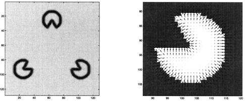
The edge indicator function g(x,y) is a non-increasing function of |∇G_σ(x,y) ★ I (x,y)|, where G_σ(x,y) is a gaussian kernel and ★ denotes the convolution. The denominator is the gradient magnitude of a smoothed version of the initial image. Thus, the value of g is closer to 1 in flat areas (|∇I| → 0) and closer to 0 in areas with large changes in image intensity: i.e., the local edge features. The minimal size of the details that are detected is related to the size of the kernel, which acts like a scale parameter. By viewing g as a potential function, we note that its minima denotes the position of edges. Also, the gradient of this potential function is a force field that always points in the local edge direction; see Fig. 2.

Figure 2.

Local edge detection: The edge map g and its spatial gradient −∇g.

To compute ∇G_σ(x,y)★I(x,y), we use the convolution derivative property ∇G_σ(x,y)★I(x,y) = ∇(G_σ(x,y)★I(x,y)) and perform the convolution by solving the linear heat equation

2

in the time interval [0, σ] with the initial condition ϕ(x,y,0) = I(x,y). We conclude this subsection by observing that there are other ways of smoothing an image as well as computing an edge indicator function or in general a feature indicator function (see refs. 8–10, 18, and 24–26).

Global Boundary Integration.

Now, consider a surface S:(x,y) → (x,y,Φ) defined in the same domain M of the image I. The differential area of the graph S in the Euclidean space is given by:

3

We will use the edge indicator g to stretch and shrink a metric appropriately chosen so that the edges act as attractors under a particular flow. With the metric g applied to the space, we have

4

Now, consider the area of the surface

5

and evolve the surface in order to (locally) minimize it. The steepest descent of Eq. 5 is obtained with usual multivariate calculus techniques and results in the following flow:

6

The first term on the right hand side is a parabolic term that evolves the surface in the normal direction under its mean curvature weighted by the edge indicator g. The surface motion is slowed down in the vicinity of edges (g → 0). The second term on the right corresponds to pure passive advection of the surface along the underlying velocity field −∇g, whose direction and strength depend on position. This term pushes/attracts the surface in the direction of the image edges. Note that g(I(x,y)) is not a function of the third coordinate; therefore, the vector field −∇g lies entirely on the (x,y) plane.

The following characterizes the behavior of the flow (Eq. 6):

• (i)  In regions of the image where edge information exists, the advection term drives the surface towards the edges. The level sets of the surface also get attracted to the edge and accumulate. Consequently, the spatial gradient increases and the surface begins to develop a discontinuity. Now, when spatial derivatives Φ_x, Φ_y ≫ 1, Eq. 6 approximates to

  7

  which is nothing but the level set flow for shape recovery (18, 27). In addition, the (parabolic) first term in Eq. 7 is a directional diffusion term in the tangent direction and limits diffusion across the edge itself.

• (ii)  The region inside the objects where g → 1,|∇g| → 0 the surface is driven by the Euclidean mean curvature motion towards a flat surface. In these regions, we observe Φ_x, Φ_y ≪ 1, and Eq. 6 approximates to:

  8

  The above equation is non-uniform diffusion equation and denotes the steepest descent of the weighted L2 norm, namely

  9

  If image gradient inside the object is actually equal to zero, then g = 1, Eq. 8 becomes a simple linear heat equation, and the flow corresponds to linear uniform diffusion.

• (iii)  We now address the regions in the image corresponding to subjective contours. In our view, subjective contours are simply continuation of existing edge fragments. As we explained before, in regions with well defined edge information, Eq. 6 causes the level curve accumulation, thereby causing an increase in the spatial gradient of Φ. Due to continuity in the surface, this edge fragment information is propagated to complete the missing boundary. The main Eq. 6 is a mixture of two different dynamics, the level set flow (7) and pure diffusion (8), and, locally, points on the Φ surface move according to one of these mechanisms. In steady state solution, the points inside the objects are characterized by pure linear diffusion while points on the boundary are characterized by the level set edge enhancing flow. The scaling of the function Φ weights the two dynamics. If Φ is “narrow range” (contains a narrow range of values), then the derivatives are small and the behavior of the flow (6) is mostly diffusive. In the opposite, when Φ is “wide range,” the behavior is mostly like level set plane curve evolution. We perform the scaling by multiplying the initial surface (x, y, Φ₀) (point-of-view surface) with a scaling factor α.

Numerical Scheme.

In this subsection, we show how to approximate Eq. 6 with finite differences. Let us consider a rectangular uniform grid in space-time (t, x, y); then, the grid consists of the points (t_n, x_i, y_j) = (nΔt, iΔx, jΔy). We denote with Φ_ijⁿ the value of the function Φ at the grid point (t_n, x_i, y_j). The first term of Eq. 6 is a parabolic contribution to the equation of motion, and we approximate this term with central differences. The second term on the right corresponds to passive advection along an underlying velocity field ∇g whose direction and strength depend on edge position. This term can be approximated by using the upwind schemes; here, we borrow the techniques described in refs. 3 and 17. In other words, we check the sign of each component of ∇g and construct one-sided difference approximation to the gradient in the appropriate (upwind) direction. With this, we can write the complete first order scheme to approximate Eq. 6 as follows:

10

where D is a finite difference operator on Φ_ijⁿ, the superscripts {−, 0, +} indicate backward, central, and forward differences, respectively, and the superscripts {x, y} indicate the direction of differentiation. We impose Dirichlet boundary conditions by fixing the value on the boundary equal to the minimum value of the point-of-view surface.

Results

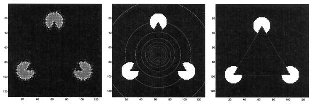
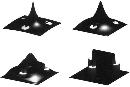
In this section, we present results of several computations aimed at performing both modal and amodal completion of objects with missing boundaries. The approach consists of a user-defined point of view or a reference surface and an edge indicator function computed as a function of the image. Different choices exist for the reference surface; we show two of them in Fig. 3. In the next examples, we use Φ₀ = α/𝒟, where 𝒟 is the distance from the initial point of view and α is a scaling factor; α = 10³ is the fixed value that we use. First, we consider the classical triangle of Kanizsa (Fig. 1) and apply the algorithm in order to perform a modal completion of the missing boundaries. We compute the edge map as shown in the left image of Fig. 4 and then choose a reference point approximately at the center of the perceived triangle (center image of Fig. 4). The evolution of the surface under the flow induced by Eq. 6 is visualized in Fig. 5. The so-called subjective surface is the steady state piece-wise linear surface shown at the end of this sequence. The triangle boundary shown in the right image of Fig. 4 is found by plotting the level set Φ̄ = {max (Φ) − ɛ} of the subjective surface. Note that, in visualizing the surface, we normalize it with respect to its maximum.

Figure 3.

Point-of-view surfaces: On the left, Φ₀ = −α𝒟, where 𝒟 is the distance function from the fixation point, and, on the right, Φ₀ = α/𝒟.

Figure 4.

Three steps of the modal completion of the triangle of Kanizsa: On the left, the edge indicator −∇g(I) is shown, in the center, a set of equispaced contour lines of the point-of-view surface are drawn, and on the right is the level set of the subjective surface that corresponds to the triangle boundary.

Figure 5.

Four time frames showing the evolution of the point-of-view surface (upper left) towards the subjective surface (bottom right). In this visualization the original image has been texture-mapped onto the surface.

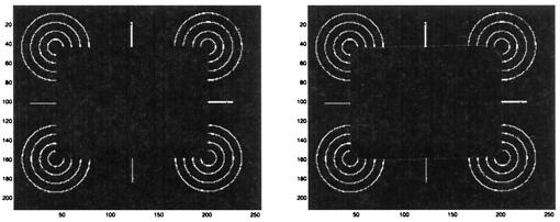
Next, we present a series of results of computing subjective surfaces. In Fig. 6, we show the subjective surface computation from an image with little or no (aligned) edge information. We render the perceived square in the final image of Fig. 6.

Figure 6.

Modal completion of an image without any aligned gradient.

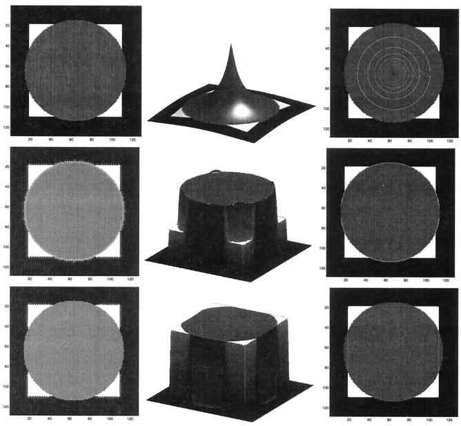
The subjective contours we have considered so far are called “modal” contours because they are “perceived” in the visual experience. Now we consider “amodal” contours that are present in images with partially occluded shapes. Consider the example of a white square partially occluded by a gray disk as shown in Fig. 7. Our goal is to recover the shapes of both the square and the disk. We employ a three-step procedure: first, we build the edge map g₁ of the image and choose a point of focus inside the disk and perform the segmentation of the gray disk O_disk. Second, we build another edge map g₂ =

so that all the image features belonging to the first object are inhibited in the new function. As the third step, we perform the modal completion of the partially occluded square by using the new edge map g₂. Again, the process is completely automatic after the initial point of reference and the entire process is shown in Fig. 7.

Figure 7.

Amodal completion of the white square partially occluded by the gray disk. In the first row the original image (left) and the point-of-view surface (center, right) are shown. In the second row, the edge map g₁ (left), the subjective surface (center), and the occluding disk boundary (right) are shown. The amodal completion of the square is shown in the third row. The new edge map g₂ (left) is obtained from the previous one by simply removing the features corresponding to the occluding object (disk). This new edge map allows the formation of a new subjective contour (center) and the square boundary (right). We use the value β = 0.3 in the edge indicator.

Echographic images are difficult candidates for shape recovery because they possess highly noisy structures, and large parts of the boundary are often found absent, thereby making shape recovery very difficult. We are interested in developing segmentation methods that deal with noncontinuous edges in extremely noisy images. In Fig. 8, we show one such computation; we use a line initialization instead of a fixation point, and the point-of-view surface is constructed to be the distance function from this initial line. The final result, a particular level set of the subjective surface is shown in the right image of Fig. 8.

Figure 8.

Segmentation of fetal echogram: Modal completion is needed to recover a large portion of the missing boundary in the dorsal section of the fetus. The original image (Left), the line of view (Center), and the segmented boundary (Right) are shown.

References

- 1.Kanizsa G. Sci Am. 1976;234:48–52. doi: 10.1038/scientificamerican0476-48. [DOI] [PubMed] [Google Scholar]
- 2.Mumford D, Shah J. Commun Pure Appl Math. 1989;XLII:577–685. [Google Scholar]
- 3.Osher S, Sethian J A. J Computat Phys. 1988;79:12–49. [Google Scholar]
- 4.Sethian J A. Commun Math Phys. 1985;101:487–499. [Google Scholar]
- 5.Sethian J A. In: Variational Methods for Free Surface Interfaces. Concus P, Finn R, editors. New York: Springer; 1987. [Google Scholar]
- 6.Malladi R, Sethian J A, Vemuri B. SPIE Proceedings on Geometric Methods in Computer Vision II. San Diego: SPIE Editors; 1993. pp. 246–258. [Google Scholar]
- 7.Caselles V, Catte' F, Coll T, Dibos F. Numer Math. 1993;66:1–31. [Google Scholar]
- 8.Sochen N, Kimmel R, Malladi R. IEEE Trans Image Processing. 1998;7:310–318. doi: 10.1109/83.661181. [DOI] [PubMed] [Google Scholar]
- 9.Kimmel, R., Malladi, R. & Sochen, N. (2000) Int. J. Comput. Vision, in press.
- 10.Malladi R, Sethian J A, Vemuri B C. IEEE Trans Pattern Anal Machine Intell. 1995;17:158–175. [Google Scholar]
- 11.Mumford D. In: Algebraic Geometry and Its Applications. Bajaj C, editor. New York: Springer; 1994. [Google Scholar]
- 12.Williams L R, Jacobs D W. Neural Comput. 1997;9:837–858. doi: 10.1162/neco.1997.9.4.837. [DOI] [PubMed] [Google Scholar]
- 13.Williams L R, Jacobs D W. Neural Comput. 1997;9:859–881. doi: 10.1162/neco.1997.9.4.837. [DOI] [PubMed] [Google Scholar]
- 14.Saund E. Proceedings of the IEEE Computer Society Conference on Computer Vision and Pattern Recognition. Vol. 2. Washington, DC: IEEE Comput. Soc.; 1999. pp. 624–630. [Google Scholar]
- 15.Marr D. Vision. San Francisco: Freeman; 1982. [Google Scholar]
- 16.Kass M, Witkin A, Terzopoulos D. Int J Comput Vision. 1988;1:321–331. [Google Scholar]
- 17.Sethian J A. Level Set Methods and Fast Marching Methods. Cambridge, U.K.: Cambridge Univ. Press; 1999. [Google Scholar]
- 18.Caselles V, Kimmel R, Sapiro G. Int J Comput Vision. 1997;22:61–79. [Google Scholar]
- 19.Sarti A, Malladi R. In: Geometric Methods in Bio-Medical Image Processing. Malladi R, editor. New York: Springer; 2000. , in press. [Google Scholar]
- 20.Chan T F, Vese L A. CAM Report 98–53. Los Angeles: Univ. of California at Los Angeles Department of Mathematics; 1998. [Google Scholar]
- 21.Gabor D. J Inst Elect Eng. 1946;93:429–457. [Google Scholar]
- 22.Lee T S. IEEE Trans Pattern Anal Machine Intell. 1996;18:959–971. doi: 10.1109/TPAMI.2011.174. [DOI] [PubMed] [Google Scholar]
- 23.Perona P. IEEE Trans Pattern Anal Machine Intell. 1995;17:488–499. [Google Scholar]
- 24.Malladi R, Sethian J A. Graph Models Image Processing. 1996;38:127–141. [Google Scholar]
- 25.Perona P, Malik J. Proc IEEE Comput Soc Workshop Comput Vision. 1987;1:16–22. [Google Scholar]
- 26.Sarti A, Mikula K, Sgallari F. IEEE Trans Med Imaging. 1999;18:453–466. doi: 10.1109/42.781012. [DOI] [PubMed] [Google Scholar]
- 27.Malladi R, Sethian J A. Proceedings of the International Conference on Computer Vision. Washington, DC: IEEE Comput. Soc.; 1998. pp. 304–310. [Google Scholar]