Stick-and-Diffuse and Caged Diffusion: A Comparison of Two Models of Synaptic Vesicle Dynamics

Abstract

Two models were recently proposed to enable us to understand the dynamics of synaptic vesicles in hippocampal neurons. In the caged diffusion model, the vesicles diffuse in small circular cages located randomly in the bouton, while in the stick-and-diffuse model the vesicles bind and release from a cellular cytomatrix. In this article, we obtain analytic expressions for the fluorescence correlation spectroscopy (FCS) autocorrelation function for the two models and test their predictions against our earlier FCS measurements of the vesicle dynamics. We find that the stick-and-diffuse model agrees much better with the experiment. We find also that, due to the slow dynamics of the vesicles, the finite experimental integration time has an important effect on the FCS autocorrelation function and demonstrate its effect for the different models. The two models of the dynamics are also relevant to other cellular environments where mobile species undergo slow diffusionlike motion in restricted spaces or bind and release from a stationary substrate.

INTRODUCTION

Fluorescence correlation spectroscopy (FCS) can probe translational, rotational, and reaction kinetics of fluorescent molecules from sub-microsecond to second timescales (1). See Rigler and Elson (2), Hess et al. (3), Schwille (4), and Thompson (5) for recent reviews. The FCS technique exploits the intensity fluctuations that occur as fluorescently labeled molecules pass through a small optical detection volume. The intensity autocorrelation function is then measured and compared with model predictions. The FCS autocorrelation has been derived for multiple diffusive reacting species (1,6), rotational diffusion of dipolar molecules (7,8), in the presence of uniform flow (9), with singlet-triplet state transitions (10), for finite detection volumes (11), and other models of dynamics and reaction kinetics.

Despite these advances, studying motion in cellular environments using FCS remains challenging. Diffusion is among only a handful of models for which FCS has an analytic solution. However, in the cell, species often interact with binding partners as well as structural elements, and rarely undergo pure diffusion. Often this motion is restricted by both cellular (11) and intracellular boundaries. If these compartments are of the order of the laser beam radius W, then the measured correlation function deviates from the expected form. Lastly, the motion of intracellular species is typically slow with correlation half-decay times τ_1/2 commonly approaching seconds, less than two orders-of-magnitude smaller than the total integration time T. This leads to a significant finite T correction to the autocorrelation function (12–14).

Recently FCS was used to study the dynamics of synaptic vesicles in hippocampal synapses (15,16). This system exhibits all the above properties that render solutions in these environments elusive. The vesicles enclose neurotransmitters, which are released in response to action potentials. The vesicles are 40 nm in size and are contained in a synaptic bouton that is only a few beam diameters in its lateral dimension (1 μm). The vesicles cannot be observed directly with light microscopy. However, they can be fluorescently labeled, the fluorescence intensity fluctuations resulting from movement in and out of the small detection volume can be measured, and the correlation function calculated. These FCS experiments were performed under a variety of conditions and supplemented by fluorescence recovery after photobleaching (FRAP) experiments. Together these experiments show:

1. Synaptic vesicles move sluggishly, taking seconds to move about the synapse. This, if interpreted as free diffusion, would imply a viscosity that is ∼2500 times larger than that for water and a diffusion constant ∼100 times larger than expected for inert particles of this size diffusing in the cell.

2. The fluctuations of the intensity are much smaller than the average intensity.

3. Synaptic vesicles move 30 times faster in the presence of the phosphatase inhibitor okadaic acid (OA), and the dynamics are well modeled by simple diffusion. This agent is thought to eliminate binding of vesicles to structural elements. Eliminating actin filaments alone, which is thought to be the dominant structural protein and source of enhanced “viscosity” in the synapse, has little effect on vesicle dynamics (1).

4. A moderate change in the system's temperature alters the correlation time dramatically, which cannot be explained by pure diffusion or any diffusionlike process that obeys the Stokes-Einstein relation. This effect is consistent with an enzyme activity.

To understand this set of observations we proposed a stick-and-diffuse model in which the vesicles bind and release from the cellular cytomatrix. The vesicles are free to diffuse when not bound (2). An alternative model based on the very slow dynamics and a very small value of normalized FCS autocorrelation function was also proposed by Jordan et al. (1). They assumed a caged diffusion model in which the vesicles undergo diffusion in circular cages within the bouton.

Although both the stick-and-diffuse and the caged diffusion models are motivated by the observations of vesicle motions in central synapses, the dynamics described by these models are common in biological systems. For instance, gene regulation and signal transduction are often accomplished by reversible binding and unbinding of a protein to its substrate, including DNA, RNA, or other proteins (17). The stick-and-diffuse model may be relevant for the diffusing protein. The caged diffusion model is relevant for the sterically restricted diffusion of biomolecules in the aqueous lumen of certain intracellular organelles, such as mitochondria and endoplasmic reticulum (18). Recent studies also reveal that lateral diffusion of membrane proteins is corralled by the underlying cytoskeleton structures (19,20) and may also be described by caged diffusion. The close relations between these important cellular processes and the dynamic behaviors ascribed by the stick-and-diffuse and the caged diffusion models provide a strong motivation for solving the models analytically.

This article is organized as follows: First, the bias due to the finite integration time T is summarized. Next, we derive analytic expressions for the autocorrelation functions for the stick-and-diffuse model and for the caged diffusion model. This allows us to compare the predictions of the two models to our experimental FCS data. We find that the stick-and-diffuse model gives a significantly better description of our experimental result while the caged diffusion model gives fits similar to that for free diffusion. Finally, a Summary is provided, where additional lines of evidence in support of the stick-and-diffuse model are discussed.

FINITE INTEGRATION TIME CORRECTION

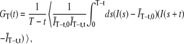
The quantity of interest in an FCS experiment is the normalized autocorrelation function. This was originally defined as (3)

(1)

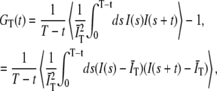
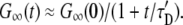
where the 〈…〉 indicates an ensemble average, I(s) is the detected intensity at time s, and 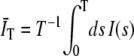is the average of the intensity over the finite integration time T. On average, , where . This leads to a finite T bias (14),

(2)

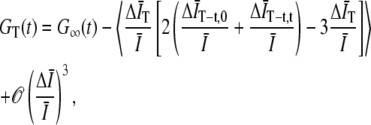
where G_∞(t) is the autocorrelation function for infinite T, and

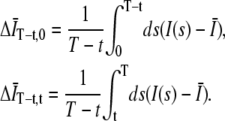(3)

This bias is always negative and can lead to G_T (t) being negative even if G_∞(t) is always positive.

More recently, Schätzel et al. (15) and Saffarian et al. (16) has pointed out the advantage of a “symmetrically” normalized autocorrelation function,

(4)

where 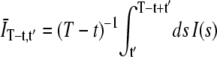. Expanding to second-order in gives

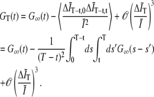(5)

To second-order in the bias in the G_T (t) comes entirely from the subtraction of and in Eq. 4. The effect of normalizing by the product instead of by in Eq. 4 contributes corrections at higher order in .

The biases for the two normalization methods are essentially the same at short times but can be significantly smaller for symmetrically normalized case at long times. An example is given in Supplement S1 in the Supplementary Material. Another important advantage of symmetric normalization is that the variance is much smaller than in the asymmetric case (15,16).

MODELS OF VESICLE DYNAMICS

Comparison of free diffusion with experimental FCS

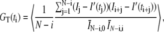
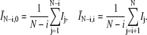
Fig. 1 shows the FCS autocorrelation function obtained in our earlier experiments on vesicle dynamics in a hippocampal synapse. (Please see Supplement S6 in the Supplementary Material and (2) for complete descriptions of the methods and materials used in this experiment, and Supplement S5 in the Supplementary Material for a detailed discussion of how the averages were performed and an estimate of uncertainties.) We used an optical spot with e^−1/2 radius W = 110 nm. (Note that W is 1/2 the more commonly quoted e⁻² beam radius.) The total integration time was limited to T = 200 s by photobleaching effects. During this integration time the total intensity decreased by ∼40–50% relative to the mean. The raw fluorescent intensity I(t) was binned to Δt = 0.01 s and then fitted to the form 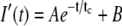, which mimics the trend-line of the fluorescence decay. The symmetrically normalized autocorrelation is given by

(6)

where the 〈…〉 indicates an ensemble average over the 39 runs and N = T/Δt. The average intensities in the denominator are

(7)

The autocorrelation function was obtained offline with t_i = iΔt. We found that the autocorrelation function was dominated by the trend-line if we did not subtract I′(t) but that the obtained autocorrelation function did not depend sensitively on the choice of the fitting form for the trend-line. We also found that fluctuations about the trend-line were not correlated with the trend-line, i.e., . See Supplement S2 in the Supplementary Material for a more detailed discussion of the effect of subtracting the trend-line. We note that while there was essentially no difference whether we normalized by or , the subtraction of the trend-line means that G_T (t_i) corresponds to the symmetrically normalized autocorrelation function.

FIGURE 1.

Panel a shows the experimental FCS autocorrelation function from Shtrahman et al. (2) for the N = 39 runs. The results are very heterogeneous with the amplitude varying by a factor of 20. Panel b shows the average autocorrelation function as discussed. The lack of noise except at long times shows that the heterogeneity in the shape of the autocorrelation function is significantly smaller than the variation in the amplitude. A detailed discussion of how the averaging is performed and the uncertainties are estimated is given in Supplement S5 in the Supplementary Material.

Our experimental data given in Fig. 1 b show that the correlation function half-decay time is ∼3 s and that G_T (t) is clearly negative at intermediate times. Fig. 2 shows the best fits of the experimental data to the different theoretical models. Fig. 2 a gives the comparison for two-dimensional free diffusion. There are two fitting parameters, the amplitude G_∞(0) and the diffusion time τ_D (see Table 1 for details of fitting parameters). The model is corrected for the finite integration time T = 200 s. The fits were performed by minimizing χ² defined as

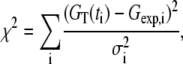(8)

where σ_i is the uncertainty of G_T at time t_i. The calculation of the uncertainty was subtle due to the large heterogeneity in the amplitude of the autocorrelation function. This is discussed in more detail in the Supplementary Material. In most FCS experiments, the autocorrelation function is obtained online resulting in times t_i that are distributed uniformly in log t. This allows one to investigate dynamics with multiple timescales. To mimic this, we prune our times which are originally uniformly distributed in time t so that we fit 51 data points uniformly distributed in log t between t = 0.01 s and t = 20 s. Following Jordan (1) the sum is restricted to i such that t_i < 20 s. The autocorrelation function is most affected by the systematic decay in the intensity for times t < 20 s (shown in Supplement S2 in the Supplementary Material). In addition to this systematic effect, the autocorrelation function for times >20 s is very noisy since the integration time is only ∼50 times larger than that of the half-decay time. Therefore, due to the larger noise and the systematic effects of the decay in intensity, the longer time data does not discriminate between different models. As a result, we focus on the early time behavior t < 20 s. The fitting values in our previous article were slightly different. Our earlier fit did not take the uncertainty into account and also used the entire autocorrelation function 0 < t < 200 s weighted by 1/t.

FIGURE 2.

The solid lines are the fits of the experimental autocorrelation function to the different models. (a) Two-dimensional free diffusion (χ² = 118). (b) Stick-and-diffuse model with two-dimensional diffusion (χ² = 10.4). (c) Caged diffusion with variable a (χ² = 99.3). (d) Caged diffusion with fixed a = 75 nm (χ² = 202).

TABLE 1.

Fitting parameters and χ² (Eq. 8) and the probability of a larger χ² (Eq. 9) for the different models

Model	χ2	Prob. larger χ2	Fitted parameters
1-D diffusion	130	3 × 10−9	G∞(0) = 0.0191 ± 0.007, τD = (1.1 ± 0.3) s
2-D diffusion	118	1 × 10−7	G∞(0) = 0.0170 ± 0.006, τD = (2.8 ± 0.6) s
2-D diffusion (two components)	50.3	0.35	G∞,1(0) = 0.0159 ± 0.006, τD1 = (3.6 ± 0.7) s G∞,2(0) = 0.0029 ± 0.0013, τD2 = (0.06 ± 0.05) s
Stick and diffuse (1-D)	21.7	0.9994	G∞(0) = 0.0176 ± 0.0002, τD = (0.085 ± 0.045) s τu = (1.8 ± 0.4) s, τb = (3.6 ± 0.5) s
Stick and diffuse (2-D)	10.4	0.999999994	G∞(0) = 0.0176 ± 0.0002, τD = (0.22 ± 0.07) s τu = (2.0 ± 0.4) s, τb = (4.2 ± 0.4) s
Caged diffusion	99.3	0.00002	G∞(0) = 0.0163 ± 0.0006, τD = (3.3 ± 1.2) s a = (360 ± 140) nm
Caged diffusion (Fixed a = 75 nm)	202	2 × 10−20	G∞(0) = 0.0158 ± 0.0006, τD = (33.5 ± 7) s

The very large values of this probability for the stick-and-diffuse model likely indicates that the uncertainty in G_T(t) is overestimated and/or the fluctuations around the fit are not independent. The diffusion constant D was the fitting parameter for the caged diffusion model. This was converted to a diffusion time using τ_D = W²/D for comparison purposes.

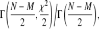
Fig. 2 a shows the fit to two-dimensional free diffusion with G_∞(0) = 0.0170 ± 0.006 and τ_D = (2.8 ± 0.6) s corresponding to D = (4.3 ± 0.9) × 10⁻³(μm)²/s with χ² = 118. The uncertainty in τ_D was obtained by determining the values of τ_D at which χ² increased by a factor (M + 1)/M, where M = 2 is the number of adjustable fitting parameters. The probability that a χ² larger than this value occurs randomly for the model is (23)

(9)

where Γ(a, x) is the incomplete γ-function, N = 51 is the number of data points in the fit, and N – M is the degrees of freedom. We have assumed the fluctuations about the fit are distributed in a Gaussian manner and are independent. The probability of a random event yielding a χ² value >118 is therefore Γ(24.5, 59)/Γ(24.5) = 1.3 × 10⁻⁷. (See Table 1 for a summary of the fitting parameters for the different models.)

We also fitted the FCS data to one-dimensional free diffusion (fit not shown). The fitting quality was approximately the same as for two-dimensional diffusion with τ_D = (1.1 ± 0.3) s corresponding to a diffusion constant D = (1.1 ± 0.3) × 10⁻²(μm)²/s and χ² = 130. The probability of a larger χ² occurring randomly is 3 × 10⁻⁹. Therefore, both one-dimensional and two-dimensional diffusion can be ruled out.

Finally, we also fit the experimental data to a two-component diffusion model. As expected, the fit is much better (χ² = 50.3) than for the single component two-dimensional diffusion but, as we will discuss later, worse than that for the stick-and-diffuse model. The probability of a larger χ² is 0.35. Therefore, two-component diffusion cannot be ruled out based on goodness of fit. However, we found a reasonable fit only occurs when the two components have widely different timescales τ_D1 = 3.5 s and τ_D2 = 0.06 s. The vesicles were synthesized by a clathrin pathway and ultra-structure studies using electron-microscopy show extremely uniform size-distribution of vesicles (24). This uniformity rules out one of the common causes of variations in the particle diffusivity; that is, the particle size distribution. Although it is not possible to completely rule out other sources of heterogeneity, it is difficult to see how either inter- or intracellular variation can lead to such a wide separation in the two diffusion times. The two component diffusion model is also difficult to reconcile with the following observations: 1), FRAP data in which exponential recovery is observed; 2), the large changes in the FCS autocorrelation functions when changing temperature; and 3), the diffusionlike behavior on application of phosphatase inhibitor okadaic acid (OA) (2). For the OA case, we found that the autocorrelation function was well fitted by single-component diffusion with a characteristic diffusion time similar to the free state diffusion time in the stick-and-diffuse model. Details of the fit to the two-component diffusion model are given in Supplement S4 in the Supplementary Material.

Stick-and-diffuse model

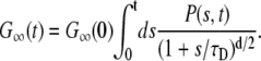
Autocorrelation function

Previous studies have established that synaptic vesicles in central nerve systems are divided into distinct functional pools. These include a readily releasable pool that is docked at an active site and a reserve pool that is remote from the active site (25). However, it is unclear from these earlier experiments how the readily releasable pool is replenished by the reserve pool after the docked vesicles are released. We addressed this kinetic question directly using FCS and FRAP by monitoring the mobility of vesicles under different conditions (2). Our experiment showed that only a small fraction of the reserve pool vesicles is mobile and therefore able to dock in the active zone, thereby playing a role in chemical transmission. We also found that the mobile pool fraction can be modulated by increasing the bath temperature and by application of the phosphatase inhibitor, OA. The diffusion constant of mobilized vesicles is 30 times larger and is the same order of free diffusion of comparable-sized objects in a cytoplasmic environment. These observations suggest that a synaptic vesicle has two intrinsic states, a state in which the vesicle is bound, presumably to the cellular cytomatrix, and a second unbound state in which the vesicle is free to diffuse. However, it is unclear whether this stick-and-diffuse model of vesicles can account for the autocorrelation function observed in our FCS measurements, and more importantly if the parameters extracted from the FCS measurements can be compared with the data from electrophysiological measurements (25). With these in mind, we set out to derive the autocorrelation function based on stick-and-diffuse phenomenology. A very rough sketch of the derivation of the FCS autocorrelation for this model was given in our previous article (2). Here we give a detailed derivation of the autocorrelation function.

We assume that the bound state is a Poisson process with unbinding rate 1/τ_b and the unbound state is a Poisson process with binding rate 1/τ_u. Therefore, the average bound and unbound intervals are τ_b and τ_u, respectively. Once unbound, the free particle has a diffusion time τ_D = W²/D in the light box formed by a tightly focused laser beam (see Supplement S6 in the Supplementary Material). The steady-state probability that a vesicle is, respectively, bound and unbound are

(10)

To calculate G_∞(t), let us assume that during time t a vesicle is free for time s₁, then bound for time b₁, then free for time s₂ and so on, such that s = s₁ + s₂ + … and t – s = b₁ + b₂ + …. The autocorrelation function at time s₁ is therefore the same as if the vesicle underwent free diffusion for time s₁, that is, , where 〈 Δr(s₁)² 〉 = 4Ds₁ is the mean-square displacement for the free diffusion process. The vesicle is frozen for time b₁, so the intensity does not change during this time and the autocorrelation function is constant: 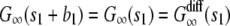. The vesicle then becomes free to diffuse for time s₂. At the end of time s₂, it is clear that the vesicle will be in the same position as if it had undergone free diffusion for time s₁ + s₂. Since the contribution of a vesicle to the autocorrelation function at time t depends only on the vesicle positions at time 0 and t, this implies that the autocorrelation function at time s₁ + b₁ + s₂ is the same as that of free diffusion at time s₁ + s₂, e.g., , where 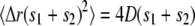is the mean-square displacement for free diffusion after time s₁ + s₂. Repeating this argument for all the segments shows that the autocorrelation function after time t depends only on the total free time s = s₁ + s₂ + … and not on the individual free segments. Furthermore the vesicle at time t is in the same position as if it had undergone free diffusion for time s so that the vesicle's contribution to the autocorrelation function at time t is the same as for a vesicle undergoing free diffusion for time s: .

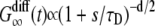Since the vesicles are independent, we can sum up the contribution from each vesicle. However all values of total free time s < t are possible. Therefore we need to sum up over all possible values of s weighted by the probability P(s, t)ds that the vesicle is free for total time between s and s + ds during time interval t:

(11)

To find P(s, t), consider the probability of having the free time s occurring in n unbound intervals with m intervening bound intervals. Note that m must be equal to n – 1, n or n + 1. Different expressions will be obtained if the vesicle is free or bound at the beginning of the interval. Summing over the different cases,

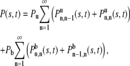(12)

where is the conditional probability density given that the vesicle is unbound at the beginning of the interval, that there is total free time s in n free intervals and total bound time t – s in m bound intervals. is the same except that the vesicle is bound at the beginning of the interval.

Start with the case where a vesicle is initially unbound. Assume there are n + 1 unbound intervals and n bound intervals where n ≥ 1. We need two conditions to find . The first is that there are n binding events in time s for a Poisson process that occurs with binding rate 1/τ_u. This probability is given by a Poisson distribution with mean value s/τ_u,

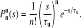(13)

The second condition is that the n^th event occurs at time t – s for a Poisson process that occurs at freeing rate 1/τ_b. This probability density is given by the Erlang distribution,

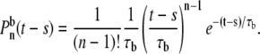(14)

Multiplying the two distributions together and including the n = 0 case gives

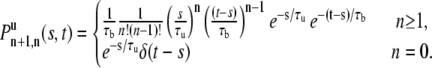(15)

For n free intervals and n bound intervals there are n – 1 binding events in total time t – s and the n^th freeing event must occur at time s:

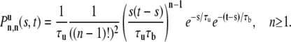(16)

Similar arguments apply when the vesicle is initially bound:

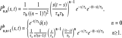(17)

Substituting Eqs. 10 and 15–17 into Eq. 12 and then into Eq. 11 gives our final result:

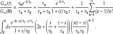(18)

The finite T autocorrelation function G_T (t) can be found using Eq. 5 once G_∞(t) is calculated.

In general, Eq. 18 must be solved numerically but the model can be easily understood in two limits:

1. τ_b ≪ τ_D ≪ τ_u: The vesicle essentially undergoes free diffusion. Only the second term in Eq. 18 is nonnegligible, and

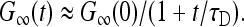(19)

1. τ_b, τ_u ≪ τ_D: There are many binding and unbinding events before the vesicle moves through the detection area. For times t ≫ τ_u, τ_b, this is effectively diffusion with a reduced diffusion constant D′ = τ_uD/(τ_u + τ_b) and/or increased diffusion time τ′_D = (τ_u + τ_b)τ_D/τ_u:

(20)

We performed direct simulations of the stick-and-diffuse model to test the theoretical expression Eq. 18 and the limiting behavior given by Eqs. 19 and 20. Results were obtained for τ_b = 0.1 s, τ_D = 1 s, and τ_u = 10 s, and also for τ_b = 0.2 s, τ_D = 2 s, and τ_u = 0.1 s to test limiting behavior. We also performed simulations for τ_b = 4.2 s, τ_D = 0.22 s, and τ_u = 2.0 s, which, as we show below, are the parameters we obtained from fitting the experimental autocorrelation function to the stick-and-diffuse model. In all cases, agreement with the theoretical expression Eq. 18 was excellent. See Supplement S3 in the Supplementary Material for more details concerning the simulation method and results.

Comparison of stick-and-diffuse model with experimental FCS

Fig. 2 b shows the fit of our FCS data to the stick-and-diffuse model. The fit was performed the same way as for the free diffusion case. We determined G_∞(t) by evaluating Eq. 18 numerically and then determined G_T(t) using Eq. 5. The four fitting parameters were τ_b = (4.2 ± 0.4) s, τ_u = (2.0 ± 0.4) s, τ_D = (0.22 ± 0.07) s, and amplitude G_∞(0) = 0.0176 ± 0.0002. The fit is significantly better than for free diffusion, with χ² = 10.4 being a factor-of-11 smaller. The probability of obtaining a χ² >10.4 is almost 1 (0.999999996). This is likely an indication that we overestimated the uncertainties of G_T(t) and/or the fluctuations are not independent (see explanation following Eq. 8).

The fitted value of the diffusion constant, D = W²/τ_D = (5.4 ± 1.6) × 10⁻²(μm)²/s, was consistent with the diffusion constant measured when OA was used to release the vesicles from the cellular cytomatrix, D ≈ 1 × 10⁻¹(μm)²/s (2). This procedure eliminates the bound state leaving only the free state. The average binding time τ_b ≈ 4 s was also consistent with the timescale observed in vesicle refilling experiments (26,27) and our measurements of the time required for the fluorescent signal to recover after photobleaching (2).

Therefore the stick-and-diffuse model predicts that, on average, a vesicle bound state lasts ∼4 s and the vesicle free state lasts on average 2 s. During the free period the vesicle can explore the entire detection area since τ_u/τ_D ≈ 10 and the intensity is essentially uncorrelated between bound states. As a result, the long time correlation function is determined by τ_b and the autocorrelation function is not very sensitive to the details of the short time dynamics as indicated by the large fractional uncertainty in τ_D. This insensitivity holds as long as the vesicle has time to explore the detection volume during an average free interval.

To further demonstrate the insensitivity of the result to the short time dynamics, we also fitted the experimental FCS autocorrelation function to the stick-and-diffuse model assuming that the diffusion is effectively one-dimensional in its free state. The fit quality is only slightly worse than for the stick-and-diffuse model in two dimensions with χ² = 21.7. The probability of a larger χ² is 0.9994 again indicating that our estimates of the uncertainty are too large. We find that τ_u = (1.8 ± 0.4) s, τ_b = (3.6 ± 0.5) s is only slightly changed from the two-dimensional result but τ_D = (0.085 ± 0.045) s is ∼65% lower. In fact we expect similar quality of fit even if the short time motion was nondiffusive as long as the dynamics are fast enough so that the vesicles can move through the detection area during a free segment and the direction of motion is uncorrelated from one free segment to the next.

Caged diffusion model

Autocorrelation function

Jordan et al. (1) proposed a caged diffusion model to explain their FCS data. They assumed that each vesicle is restricted to a circular cage of radius a. The vesicle is assumed to undergo diffusion with diffusion constant D inside this circular cage. For simplicity, the cages are assumed to be located randomly within the bouton and the vesicles are assumed to be independent. In this section we will obtain an expression for the FCS autocorrelation function for the caged diffusion model and compare the results with our FCS data.

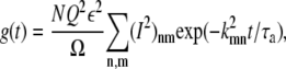
Consider a single vesicle in a cage of radius a with the cage center at R. The nonnormalized autocorrelation function g(t) is defined by

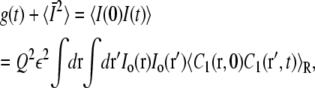(21)

where Q is the quantum efficiency, ε is the absorbance, and I_o(r) is the laser beam intensity profile. The brackets 〈〉_R indicate an average over all initial conditions r₀ inside the cage. The concentration C₁(r, t) is the solution to the diffusion equation

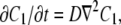(22)

corresponding to a single particle at r_o at t = 0 with no flux boundary conditions at the edge of the cage. A cage centered at R with a beam centered at the origin is equivalent to having a cage centered at the origin and the beam centered at r = – R. Making this shift, Eq. 21 becomes

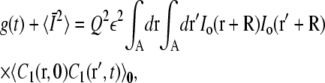(23)

where the integrals are restricted over the area A = πa² of the cage. Assuming a Gaussian beam profile and N independent particles in N cages centered at R_i, i = 1, …, N, gives

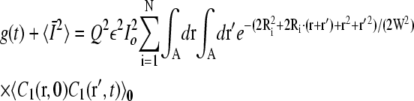(24)

The ensemble average now corresponds to an average over cage positions R_i. Performing this average gives

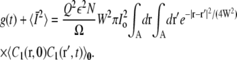(25)

We have assumed that the area of the bouton Ω is much larger than the detection area and that the positions of the cages are not correlated.

Solving the diffusion equation (Eq. 22) in cylindrical coordinates with no flux boundary condition 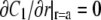gives 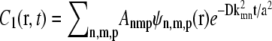where A_nmp are constants that depend on the initial position of the vesicle and the functions ψ_n,m,p(r) form the orthonormal basis for the Laplacian in cylindrical coordinates (28). The basis functions factor into a radial and angular part, Ψ_n,m,p(r) = ψ_n,m(r)Θ_m,p(θ),

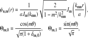(26)

where J_m(x) is the m^th Bessel function of the first kind and k_mn is the (n + 1)^th zero of the derivatives of J_m(x), i.e., .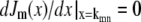

Taking C₁(r, 0) = δ(r – r_o) and then averaging over all initial positions r_o inside the cage of radius a gives the concentration-concentration correlation:

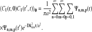(27)

The autocorrelation function becomes

(28)

where the sum is over all n and m except for the term in which both n = 0 and m = 0. Since k₀₀ = 0, this term corresponds to the constant term in Eq. 21. The time required for the vesicle to diffuse through the cage is τ_a = a²/D and

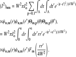(29)

Here F_m(y) is the angular part of the integration:

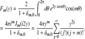(30)

Introducing the rescaling x = k_mnr/a gives

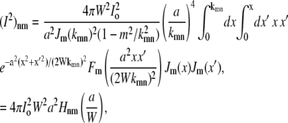(31)

where the function H_nm(a/W) is only a function of the ratio a/W. Equation 28 then becomes

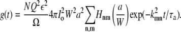(32)

Therefore the ratio g(t)/g(0) = G_∞(t)/G_∞(0) = f(t/τ_a, a/W) is a function only of t/τ_a and a/W. Fig. 3 a shows this ratio as a function over t/τ_a for different a/W. The symbols are results of direct simulation of the caged diffusion model. There is an excellent match between the analytical and the simulation results.

FIGURE 3.

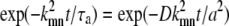
G_∞(t)/G_∞(0) for the caged diffusion model: (a) G_∞(t)/G_∞(0) depends only on the ratios a/W and t/τ_a. The lines are the theoretical results (Eq. 32) and the symbols are results from direct simulation of the caged diffusion model. Results are shown for a/W=1/4 (Δ), 2 (□), and 5 (○). (b) For a ≫ W, the cage diffusion model (solid) behaves similar to τ_D = W²/D (dashed). (c) The decay is approximately single-exponential for with decay time τ = a²/(3.39 D). The squares are just for the m = 1, n = 0 term in Eq. 32.

The behavior of the caged diffusion model can be easily understood in two limits:

1. a/W ≫ 1: The cage is irrelevant since it is much larger than the beam radius. The dynamics is the same as free diffusion with a diffusion time τ_D = W²/D = (W/a)²τ_a. (In this limit, the sums in Eq. 32 can be converted to an integral over q = k_mn/a. The exponential becomes exp(−Dq²t), thereby giving free diffusion.) Fig. 3 b shows a comparison of the caged diffusion model for a/W = 5 with two-dimensional free diffusion. The curves coincide for t/τ_D < 4. At longer times the finite cage size becomes important. The effect is similar to the finite sample size corrections given by Gennerich and Schild (13).

2. : The autocorrelation function is essentially independent of the ratio a/W as long as . As shown in Fig. 3 c, G_∞(t) is dominated by the m = 1, n = 0 term in Eq. 32 and , where . This is the slowest decaying mode since . The decay is a good single exponential for a/W as large as 1.

Comparison of caged diffusion with experimental FCS

Jordan et al. (1) compared their FCS power spectrum with simulations of the caged diffusion model. They found that the experimental power spectrum very roughly matched their simulations when they assumed a beam radius of ∼85 nm, a cage size of between 50 and 100 nm and a very small diffusion constant of ∼5 × 10⁻⁵ (μm)²/s. Fig. 2 c shows the best fit of our experimental FCS autocorrelation to the caged diffusion model with our beam radius W = 110 nm. The fitting parameters were a = (360 ± 140) nm, D = (3.7 ± 1.5) × 10⁻³(μm)²/s, and G_∞(0) = 0.0164 ± 0.0006. The fit is significantly worse than for the stick-and-diffuse model. We find χ² = 99.3 with the probability of a larger χ² being 0.000019. This value of χ² is only slightly smaller than the fits to free diffusion. In particular, the diffusion time τ_D = W²/D ≈ (3.3 ± 1.3) s is close to the diffusion time, τ_D = (2.7 ± 0.7) s, obtained from the fit to two-dimensional free diffusion. This is because a/W ≈ 3.5 so the finite cage size has little effect except at late times.

Our best fit parameters are in a different regime from those obtained by Jordan et al. (1). In their case they found and a much smaller diffusion constant. Therefore we also fit the caged diffusion model with the cage radius fixed at a = 75 nm. Fig. 2 d shows the best fit with a = 75 nm and W = 110 nm fixed. The fit is poor with χ² = 202, approximately twice that of this model when we allow a to be adjusted. The fitting parameters were D = (3.6 ± 0.8) × 10⁻⁴ (μm)²/s and G_∞(0) = (0.0161 ± 0.0006). The diffusion constant is approximately seven times larger than the value obtained in Jordan et al. (1). However, the functional form is not very dependent on a/W for a < W so fixing a to 50 nm gives a similar fit with D very similar to the value they obtained.

SUMMARY

In summary, we have obtained analytic expressions for the intensity autocorrelation functions for two proposed models of vesicle dynamics in central synapses, the stick-and-diffuse model and the caged diffusion model. We find that the stick-and-diffuse model gives a good fit to the experimental data, while the fit to the caged diffusion model is poor and similar to that of free diffusion. The better fit alone does not in itself indicate that the stick-and-diffuse model is a valid description of the dynamics. However, several independent experiments provide additional support for the stick-and-diffuse model. First, the free diffusion time (τ_D ≈ 0.2 s, D ≈ 0.05 (μm)²/s) agrees well with the diffusion time measured in FCS experiments on synapses exposed to OA (τ_1/2 ≈ 0.1 s, D ≈ 0.1 (μm)²/s), where vesicles are unbound and diffuse freely. These dynamics agree reasonably well with the diffusion time measured for inert particles of this size in cells (29) as well as synaptic vesicles in synapses that lack synapsin, a major vesicle binding protein (30,31). In contrast, the caged diffusion model predicts a diffusion time which is ∼300-times larger. Next, changing the temperature of the system by several degrees dramatically alters the vesicle dynamics. This is not consistent with pure or caged diffusion, and is indicative of an enzymatic process such as phosphorylation-dependent binding. Lastly, the stick-and-diffuse model predicts both the FRAP and the previously published electrophysiological refilling results (26,27), with the sticking time τ_b consistent with the exponential recovery time. These features cannot be addressed by the caged diffusion model, which predicts no fluorescence recovery or vesicle refilling.

Therefore the stick-and-diffuse model is consistent with existing kinetic measurements of vesicle dynamics in synapses. The model makes specific predictions about how the vesicles move about in synapses and may be further tested in future experiments using single-molecule techniques. The analytic expressions for the autocorrelation function may also be useful for analyzing FCS data in other biological systems, which is suspected of undergoing bind-and-diffuse dynamics or caged diffusion dynamics.

SUPPLEMENTARY MATERIAL

An online supplement to this article can be found by visiting BJ Online at http://www.biophysj.org.

References

- 1.Magde, D., E. Elson, and W. Webb. 1972. Thermodynamic fluctuations in a reacting system—measurement by fluorescence correlation spectroscopy. Phys. Rev. Lett. 29:705–708. [Google Scholar]
- 2.Rigler, R., and E. Elson. 2001. Fluorescence Correlation Spectroscopy, Theory and Application. Springer-Verlag, Berlin.
- 3.Hess, S., S. Huang, A. Heikal, and W. Webb. 2002. Biological and chemical applications of fluorescence correlation spectroscopy: a review. Biochemistry. 41:697–705. [DOI] [PubMed] [Google Scholar]
- 4.Schwille, P. 2001. Fluorescence correlation spectroscopy and its potential for intracellular applications. Cell Biochem. Biophys. 34:383–408. [DOI] [PubMed] [Google Scholar]
- 5.Thompson, N., A. Lieto, and N. Allen. 2002. Recent advances in fluorescence correlation spectroscopy. Curr. Opin. Struct. Biol. 12:337–378. [DOI] [PubMed] [Google Scholar]
- 6.Magde, D., E. Elson, and W. Webb. 1974. Fluorescence correlation spectroscopy. II. An experimental realization. Biopolymers. 13:29–61. [DOI] [PubMed] [Google Scholar]
- 7.Ehrenberg, M., and R. Rigler. 1974. Rotational Brownian motion and fluorescence intensity fluctuations. Chem. Phys. 4:390–401. [Google Scholar]
- 8.Aragón, S., and R. Pecora. 1975. Fluorescence correlation spectroscopy and Brownian rotational motion. Biopolymers. 14:119–138. [Google Scholar]
- 9.Magde, D., and E. Elson. 1978. Fluorescence correlation spectroscopy. III. Uniform translation and laminar flow. Biopolymers. 17:361–376. [Google Scholar]
- 10.Widengren, J., U. Mets, and R. Rigler. 1995. Fluorescence correlation spectroscopy of triplet states in solution: a theoretical and experimental study. J. Phys. Chem. 99:13368–13379. [Google Scholar]
- 11.Gennerich, A., and D. Schild. 2000. Fluorescence correlation spectroscopy in small cytosolic compartments depends on the diffusion model used. Biophys. J. 79:3294–3306. [DOI] [PMC free article] [PubMed] [Google Scholar]
- 12.Jakeman, E., E. Pike, and S. Swain. 1971. Statistical accuracy in the digital autocorrelation of photon counting fluctuations. J. Phys. A. 4:517–534. [Google Scholar]
- 13.Schätzel, K., M. Drewel, and S. Stimac. 1989. Photon correlation measurements at large lag times: improving statistical accuracy. J. Mod. Opt. 35:711–718. [Google Scholar]
- 14.Saffarian, S., and E. L. Elson. 2003. Statistical analysis of fluorescence correlation spectroscopy: the standard deviation and bias. Biophys. J. 84:2030–2042. [DOI] [PMC free article] [PubMed] [Google Scholar]
- 15.Jordan, M., E. Lemke, and J. Klingauf. 2005. Visualization of synaptic vesicle movement in intact synaptic boutons. Biophys. J. 89:2091–2102. [DOI] [PMC free article] [PubMed] [Google Scholar]
- 16.Shtrahman, M., C. Yeung, D. Nauen, G. q. Bi, and X. Wu. 2005. Probing vesicle dynamics in single hippocampal synapses. Biophys. J. 89:3615–3627. [DOI] [PMC free article] [PubMed] [Google Scholar]
- 17.Lippincott-Schwartz, J., E. Snapp, and A. Kenworthy. 2001. Studying protein dynamics in living cells. Nat. Rev. Mol. Cell Biol. 2:444–456. [DOI] [PubMed] [Google Scholar]
- 18.Verkman, A. 2002. Studying protein dynamics in living cells. Trends Biochem. Sci. 27:27–33.11796221 [Google Scholar]
- 19.Brown, F., D. Leitner, J. McCammon, and K. Wilson. 2000. Studying protein dynamics in living cells. Biophys. J. 78:2257–2269. [DOI] [PMC free article] [PubMed] [Google Scholar]
- 20.Kusumi, A., C. Nakada, K. Ritchie, K. Murase, K. Suzuki, H. Murakoshi, R. S. Kasai, J. Kondo, and T. Fujiwara. 2005. Paradigm shift of the two-dimensional continuum fluid to the partitioned fluid: high-speed single-molecule tracking of membrane molecules. Annu. Rev. Biophys. Biomol. Struct. 34:351–378. [DOI] [PubMed] [Google Scholar]
- 21.Reference deleted in proof.
- 22.Reference deleted in proof.
- 23.Press, W., B. Flannery, S. Teukolsky, and W. Vetterling. 2002. Numerical Recipes. Cambridge University Press, London.
- 24.Sudhof, T. 1995. The synaptic vesicle cycle: a cascade of protein-protein interactions. Nature. 375:645–653. [DOI] [PubMed] [Google Scholar]
- 25.Schikorski, T., and C. Stevens. 2001. Morphological correlates of functionally defined synaptic vesicle populations. Nat. Neurosci. 4:391–395. [DOI] [PubMed] [Google Scholar]
- 26.Stevens, C., and J. Wesseling. 1999. Identification of a novel process limiting the rate of synaptic vesicle cycling at hippocampal synapses. Neuron. 27:539–550. [DOI] [PubMed] [Google Scholar]
- 27.Morales, M., M. Colicos, and Y. Yoda. 2000. Actin-dependent regulation of neurotransmitter release at central synapses. Neuron. 27:539–550. [DOI] [PubMed] [Google Scholar]
- 28.Farlow, S. 1993. Partial Differential Equations for Scientist and Engineers. Dover, Mineola, New York.
- 29.Luby-Phelps, K., P. E. Castle, L. D. Taylor, and F. Lanni. 1987. Hindered diffusion of inert tracer particles in the cytoplasm of mouse 3t3 cells. Proc. Natl. Acad. Sci. USA. 84:4910–4913. [DOI] [PMC free article] [PubMed] [Google Scholar]
- 30.Holt, M., A. Cooke, A. Neef, and L. Lagnado. 2004. High mobility of vesicles supports continuous exocytosis at a ribbon synapse. Curr. Biol. 14:173–183. [DOI] [PubMed] [Google Scholar]
- 31.Rea, R., J. Li, A. Dharla, E. S. Levitan, P. Sterling, and R. H. Kramer. 2004. Streamlined synaptic vesicle cycle in cone photoreceptors terminals. Neuron. 41:755–766. [DOI] [PubMed] [Google Scholar]