Classical versus Stochastic Kinetics Modeling of Biochemical Reaction Systems

Abstract

We study fundamental relationships between classical and stochastic chemical kinetics for general biochemical systems with elementary reactions. Analytical and numerical investigations show that intrinsic fluctuations may qualitatively and quantitatively affect both transient and stationary system behavior. Thus, we provide a theoretical understanding of the role that intrinsic fluctuations may play in inducing biochemical function. The mean concentration dynamics are governed by differential equations that are similar to the ones of classical chemical kinetics, expressed in terms of the stoichiometry matrix and time-dependent fluxes. However, each flux is decomposed into a macroscopic term, which accounts for the effect of mean reactant concentrations on the rate of product synthesis, and a mesoscopic term, which accounts for the effect of statistical correlations among interacting reactions. We demonstrate that the ability of a model to account for phenomena induced by intrinsic fluctuations may be seriously compromised if we do not include the mesoscopic fluxes. Unfortunately, computation of fluxes and mean concentration dynamics requires intensive Monte Carlo simulation. To circumvent the computational expense, we employ a moment closure scheme, which leads to differential equations that can be solved by standard numerical techniques to obtain more accurate approximations of fluxes and mean concentration dynamics than the ones obtained with the classical approach.

INTRODUCTION

The design of predictive models of cellular regulation is an important problem in computational systems biology. The majority of models published in the literature assume that cells are well-stirred, homogeneous biochemical reaction systems at thermal equilibrium, an assumption that we also follow in this article. A widely used approach to modeling cellular regulation characterizes the dynamic evolutions of molecular concentrations by deterministic first-order ordinary differential equations, known as chemical kinetics equations (CKEs) (1). However, to take into account that reactions in cells occur by random collisions of reactant molecules, we must employ a stochastic approach to modeling cellular regulation. A popular approach characterizes the dynamic evolution of the joint probability mass function of the state of cellular regulation by a first-order partial differential equation known as the chemical master equation (CME) (2–4). This leads to a modeling methodology that has been employed in several biological settings with remarkable success (5–9).

It has been increasingly recognized that cellular regulation should be studied at the level of single cells. Despite a growing effort to develop experimental methods for observing biochemical activities in single cells (10–12), these methods can only be used to simultaneously observe a limited number of molecular dynamics. Most experimental techniques used today estimate molecular concentrations in tissues containing a large number of cells (13,14). As a consequence, appreciable research activity is focused on studying the aggregate behavior of cellular regulation in a large population of cells.

For the purpose of this work, we may assume that a tissue is composed of K genetically identical cells that express the same set of genes independently from each other. This is a convenient albeit reasonable approximation, since it frees us from modeling tissue inhomogeneities and biological effects due to complex interactions among cells. We may model cellular activities in each cell by a stochastic biochemical reaction system that consists of N molecular species and use the random variable X_nk(t) to denote the number of molecules of the n^th species present in the k^th cell at time t. Since cellular regulation is observed by pooling together molecules extracted from all cells in the tissue, we may characterize its state at time t by the molecular concentrations Y_n(t) = (X_n1(t) + X_n2(t) + ··· + X_nK(t))/KAV, where V is the cellular volume and A = 6.0221415 × 10²³ mol⁻¹ is the Avogadro constant. The mean value and variance of Y_n(t) are given by E(Y_n(t)) = μ_X,n(t)/AV and Var(Y_n(t)) = v_X,nn(t)/KA²V², where μ_X,n(t) and v_{X, nn}(t) are the mean and variance of X_nk(t), respectively. This implies that the mean value of the molecular concentration Y_n(t) of the n^th species is independent of the number of cells in the tissue, whereas its variance tends to zero as the number of cells grows to infinity (provided that the variance v_X,nn(t) is finite). As a consequence, we may approximately characterize cellular regulation in a large population of cells by the mean concentration vector

(1)

where denotes the N × 1 mean vector with elements μ_X,n(t), n = 1, 2, …, N.

An important question that arises here is whether the molecular concentration dynamics predicted by the CKEs coincide with the mean concentration dynamics predicted by the underlying CME and Eq. 1. It turns out that, given the CME, we can uniquely construct the corresponding CKEs and vice versa. Therefore, we may expect that the two approaches lead to the same dynamics. However, by analyzing a number of simple chemical reactions such as 2A → B, A + B → C, A → B, A → B → C, 2A → B → C, and , it was previously shown in the literature (15–17) that this may not be true in general. A notable exception occurs at the thermodynamic limit, in which the number of molecules and cellular volume tend to infinity while the molecular concentrations remain finite, or when all reaction mechanisms are linear. However, both of these cases are clearly not realistic.

In Zheng and Ross (18), they extended the previous work by focusing on the autocatalytic cubic Schlögl model , . These investigators noted that differences between classical and stochastic chemical kinetics are due to a coupling of correlation effects with system nonlinearities. By focusing on parameter values that lead to the same stationary states (concentrations of the molecular intermediate B) for both models, they showed that the deterministic model may result in quantitatively different transient behavior for the mean concentration of B than the corresponding stochastic model, with the maximum deviation between the concentration trajectories decreasing as the model parameters are modified toward a linear kinetic mechanism.

In view of the fact that cellular regulation is controlled by a complex network of biochemical reactions, it is necessary to investigate the relationship between classical and stochastic chemical kinetics in a more general setting than the one considered in the literature (15–18). In this article, we derive fundamental relationships between the two approaches for a biochemical reaction system that consists of elementary (monomolecular or bimolecular) irreversible reactions. We can use this system to model any set of biochemical reactions, since we can decompose any reaction that involves more than two molecules (a rare possibility in practice) into a cascade of bimolecular reactions and split a reversible reaction into two separate irreversible reactions (19). We have chosen to illustrate our results by employing two reaction mechanisms: a unidirectional dimerization and a quadratic autocatalator with positive feedback. These mechanisms allow us to clearly demonstrate that intrinsic stochastic fluctuations may appreciably influence the qualitative and quantitative behavior of cellular regulation and to analytically investigate the origins of such influence. Note, however, that our approach is very general and can be applied to more complex regulatory mechanisms as well.

In this article, we show that the mean concentration dynamics predicted by the CME are governed by first-order ordinary differential equations similar to the ones obtained by classical chemical kinetics, expressed in terms of the stoichiometry coefficients and the time-dependent fluxes of the underlying reactions. However, the flux is now decomposed into a macroscopic and a mesoscopic term. The macroscopic term is analytically identical to the classical flux and accounts for the effect of mean reactant concentrations on the rate of product synthesis, whereas the mesoscopic term accounts for the effect of statistical correlations among interacting reactions. When all mesoscopic fluxes are zero, a situation that occurs when the biochemical reaction system consists of only monomolecular reactions (which leads to linear reaction mechanisms), the concentration dynamics predicted by the CKEs will be identical to the mean concentration dynamics predicted by the CME. However, and by using the two aforementioned examples, our analytical and numerical investigations show that nonzero mesoscopic fluxes may induce appreciable qualitative and quantitative differences in transient and stationary system behavior from that predicted by classical chemical kinetics. In addition to the conclusions reached by Zheng and Ross (18), we show that the mean concentration dynamics predicted by the CME may converge to different stationary values than those predicted by the CKEs, thus supporting the fact that intrinsic stochastic fluctuations may play an important role in determining a cell's phenotype by quantitatively influencing cell regulation at steady state. Moreover, we analytically and numerically demonstrate that intrinsic stochastic fluctuations may also affect the epigenetic properties of cell regulation in a qualitative manner by introducing novel modes of stationary behavior not accounted for by the CKEs. Hence, a sufficiently accurate model of mean concentration dynamics must necessarily include all mesoscopic fluxes in its formulation. These developments provide a theoretical understanding of the role that intrinsic stochastic fluctuations may play in inducing biochemical function.

The mesoscopic fluxes cannot be evaluated analytically. We can estimate them by Monte Carlo simulation, but the resulting method is computationally intensive in most cases of interest. To circumvent the computational expense, we employ a moment closure scheme that allows us to approximate the underlying covariances (and thus the mesoscopic fluxes) by first-order ordinary differential equations that are similar to the CKEs and can be solved by standard numerical techniques. We show that, at least for the quadratic autocatalator, this approximation leads to more accurate predictions of fluxes and mean concentration dynamics than the CKEs.

We should mention that, in a recent work (20), Samoilov et al. have used a simple example (an enzymatic futile cycle) to analytically and numerically demonstrate that extrinsic stochastic fluctuations in biochemical reaction systems may also produce dynamic behavior not accounted for by classical chemical kinetics. Our work is complementary to theirs, since it focuses on the effects of intrinsic stochastic fluctuations on system behavior. Moreover, it supports, both analytically and computationally, the general belief that stochastic fluctuations may play an important role in determining biological function in cells and, therefore, must be accounted for by computational models of cellular regulation.

BIOCHEMICAL REACTION SYSTEMS

Deterministic description

In this article, we consider a well-stirred biochemical reaction system at thermal equilibrium that consists of M elementary (monomolecular or bimolecular) irreversible reaction channels. By assuming that the system contains N molecular species, we may characterize its state at time t ≥ 0 by an N × 1 deterministic vector q(t) whose dynamic evolution is governed by the following CKEs (1):

(2)

In Eq. 2, is the N × M stoichiometry matrix of the underlying biochemical reactions. Moreover, ρ(t) is an M × 1 (time-dependent) vector with elements ρ_m(t) = (1/V) dξ_m(t)/dt, where ξ_m(t) is the extent of the m^th reaction, defined as the amount (in moles) of a species produced or consumed by the m^th reaction during the time interval [0,t), divided by the corresponding stoichiometric coefficient. Note that ρ_m(t) is the rate of change in the extent of reaction per unit volume at time t and, hence, it quantifies the reaction rate of the m^th reaction. These parameters are frequently referred to as time-dependent fluxes (velocities of molecular flow) and play a fundamental role in the analysis of biochemical reaction systems (1). The mass action rate law implies that the m^th element of ρ(t) is given by

(3)

where κ_m is the reaction rate constant of the m^th reaction and ψ_m(q) is a product of the reactant concentrations of the m^th reaction, given by

(4)

Note that in classical chemical kinetics it is assumed that molecular concentrations are appreciably larger than 1/AV, in which case for bimolecular reactions with identical reactants. To account for the possibility that some molecular concentrations may be comparable to 1/AV, we set in this article ψ_m(q) = q_n(q_n – 1/AV).

Although it is commonly believed that q(t) provides a sufficient approximation to the mean concentration vector u(t), given by Eq. 1, because of stochastic fluctuations in biochemical activity, this may not be true. Moreover, the derivation of Eq. 2 requires that the numbers of molecules in the system are very large compared to 1. Otherwise, q(t) will not be a continuous function of t and differentiation of q(t) will not be possible. Therefore, we may not be able to justify the CKEs when modeling biochemical reaction systems with appreciable stochastic fluctuations and small numbers of reactant molecules. In view of the fact that reactions occur by random collisions of reactant molecules, it is intuitive to believe that it will be more appropriate if we employ a stochastic approach.

Stochastic description

If we use a stochastic biochemical reaction system to model cellular regulation in single cells, then the mean molecular concentrations u(t), given by Eq. 1, will satisfy the system of first-order differential equations

(5)

where ν(t) is an M × 1 (time-dependent) flux vector with elements ν_m(t) = (1/V) dχ_m(t)/dt, and χ_m(t) is the extent of the m^th reaction at time t, which is now defined as the mean degree of advancement (DA) of the m^th reaction at time t divided by the Avogadro number (see Appendix A for a brief review of stochastic chemical kinetics). Notably, the flux ν_m(t) of the m^th reaction is the rate of change in its mean DA per unit volume divided by the Avogadro number.

Equation 5 is similar to the CKEs with one important difference. The m^th element ν_m(t) of the flux vector ν(t) is now given by

(6)

where

(7)

as in the deterministic case, and (see Appendix A)

(8)

In Eq. 8, η_m,kl is the second-order partial derivative of the propensity function of the m^th reaction with respect to the DAs of the k^th and l^th reactions, whereas, v_{Z, kl}(t) is the covariance between the DAs of those reactions. We refer to ρ_m(t) as the macroscopic flux and to θ_m(t) as the mesoscopic flux of the m^th reaction. Clearly, the macroscopic flux accounts for the effect of mean reactant concentrations on the rate of product synthesis, whereas the mesoscopic flux accounts for the effect of statistical correlations among interacting reactions on that rate. Because the propensity functions are at most quadratic functions of the DAs (see Appendix A), the mesoscopic flux of a given reaction depends only on the (nonzero) Hessian elements of the propensity function of that reaction and on the corresponding DA covariances. As a consequence of Eq. 8, the mesoscopic flux of a monomolecular reaction will be zero, since the propensity function of such reaction will be linear and the corresponding Hessian matrix will be zero (i.e., η_m,kl = 0, for every k, l). However, this may not be true for the mesoscopic flux of a bimolecular reaction, whose value will depend on the DA covariances between reactions that affect the molecular population of one reactant species and reactions that affect the population of the other reactant species.

If all reactions are monomolecular, the biochemical reaction system will be linear (i.e., all propensity functions will be linear). In this case, the second-order partial derivatives of the propensity functions with respect to the DAs will be zero, which, together with Eq. 8, implies that θ_m(t) = 0, for every m (since η_m,kl = 0, for every m, k, l). Hence, when all reactions are monomolecular, Eq. 5 is identical to Eq. 2 of classical chemical kinetics. This result was derived in Gillespie (21).

Equations 5–8 extend the classical CKEs 2 and 3 to account for intrinsic stochastic fluctuations in biochemical activity and are an exact consequence of the conservation of mass and the CME underlying the biochemical reaction system (Eqs. 21 and 27). Note that

(9)

where

(10)

We refer to these equations (and Eqs. 5–8) as statistical chemical kinetics equations (SCKEs), where we use the term “statistical” to emphasize that the equations account for correlations among reactions. Like the CKEs, the SCKEs provide a macroscopic description of a biochemical reaction system. However, this description is now controlled by the mesoscopic behavior of the system through the forcing term ɛ(t). If ɛ(t) were known for every t ≥ 0, then we could evaluate u(t) by integrating Eq. 9 using standard numerical techniques. However, this is not true and u(t) must be estimated by computationally intensive Monte Carlo simulation using the Gillespie algorithm (22). In an effort to circumvent this computational expense, we later discuss a method that allows us to approximately evaluate u(t) by numerically integrating an appropriately derived system of first-order ordinary differential equations.

Deterministic versus stochastic description

Equation 9 reveals that intrinsic stochastic fluctuations may influence the mean concentration dynamics u(t) through the mesoscopic forcing term ɛ(t). This fact is not considered by the CKEs and its importance should not be underestimated. If, for some species n, ɛ_n(t) ≠ 0, for every t ≥ 0, then at least one function ψ_m will be quadratic, where m is a reaction that consumes or produces the n^th molecular species, and the n^th SCKE will therefore be nonlinear. Indeed, if ψ_m is linear, for any reaction m that consumes or produces the n^th molecular species, then its second-order partial derivative η_m,kl will be zero, for every k, l, which implies that θ_m(t) = 0, by virtue of Eq. 8. Since the mesoscopic forcing term ɛ_n(t) is given by Eq. 10, this implies that ɛ_n(t) = 0 for every t ≥ 0, which contradicts our assumption that ɛ_n(t) ≠ 0 for every t ≥ 0. By combining this observation with the fact that a nonzero forcing term may substantially affect the solution of a nonlinear differential equation, we may expect that nonzero mesoscopic forcing terms could appreciably affect the mean behavior of a nonlinear biochemical reaction system.

It is clear from our previous discussion that we may use the CKEs to characterize the mean concentration dynamics if and only if, at any time t ≥ 0, the mesoscopic flux vector θ(t) is in the null space of the stoichiometry matrix . In this case, , for every t ≥ 0, and the SCKEs will be reduced to the CKEs. Eq. 8 suggests that this will happen if all underlying reactions are monomolecular (see also (18,21)). We may also use the CKEs when all covariances are zero, a condition that will be satisfied in the thermodynamic limit. However, most biochemical reaction systems of interest are nonlinear and there is no way to know a priori whether the covariances are zero or, more generally, whether θ(t) is in the null space of . Therefore, to account for the influence of nonzero mesoscopic fluxes on system dynamics, we must include them in the formulation.

Numerical example

To provide a simple illustration of our discussion so far, we consider the following unidirectional dimerization reaction,

(11)

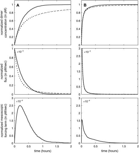
with specific probability rate constant c₁, initialized with S molecules P and S molecules Q (see Appendix B for details). In Fig. 1, we depict the normalized (with respect to the steady-state dimer concentration s = S/AV) dimer concentration and flux dynamics, predicted by the underlying SCKE (solid lines) versus the ones predicted by the corresponding CKE (dotted lines), for S = 1, in Fig. 1 A, and S = 10, in Fig. 1 B. We also depict the dynamics of the normalized mesoscopic forcing term. We have estimated the concentrations, fluxes, and forcing terms by Monte Carlo simulation using the Gillespie algorithm (22,23), and calculated the CKE concentrations and fluxes analytically (see Eq. 38). It turns out that, as t→∞, both models converge to the same steady-state concentration s.

FIGURE 1.

Normalized dimer accumulation in the unidirectional dimerization reaction, given by Eq. 11, predicted by the SCKEs (solid lines) and CKEs (dotted lines). The dynamics obtained by the SCKEs have been computed by Monte Carlo simulation using the Gillespie algorithm, whereas the dynamics obtained by the CKEs have been computed analytically from Eq. 38. The system is initialized with (A) one molecule P and one molecule Q, (B) 10 molecules P, and 10 molecules Q. The associated normalized flux and mesoscopic forcing term dynamics are depicted as well. Parameters used are c₁ = 10⁻³ s⁻¹, V = 2 pL, and K = 6000 cells.

When the initial number of reactant molecules is very small (e.g., when S = 1 in Fig. 1 A), the CKE concentration dynamics do not match the SCKE dynamics obtained by Monte Carlo simulation. According to the results depicted in Fig. 1 A, small differences in flux dynamics may lead to substantial differences in concentration dynamics. However, a sufficient increase in the initial number of reactant molecules (e.g., by tenfold in Fig. 1 B) may drastically alleviate this difference. For sufficiently large S (S ≥ 100) the flux and concentration dynamics are virtually identical (data not shown).

The observed differences are due to the mesoscopic forcing term, which coincides in this case with the mesoscopic flux of the reaction. Since all reactants are eventually transformed into dimers, the mesoscopic forcing term tends to zero as t→∞. Its magnitude and rate of convergence to zero affect the SCKE concentration dynamics and the time it takes for the system to reach steady state. Because the flux is given by Eq. 37, larger values of the mesoscopic forcing term will promote faster reaction rates and thus faster relaxation to steady state (for this example, the mesoscopic forcing term is nonnegative). Fig. 1 shows that, when S = 1, the mesoscopic forcing term converges to zero slower than when S = 10. Our simulations show that the response predicted by the SCKE reaches steady state at ∼2 h, whereas the response predicted by the CKE requires substantially more time (∼24 h) to reach steady state. This example provides an analytical justification, by means of the mesoscopic forcing term, of a previously recognized fact that intrinsic stochastic fluctuations in biochemical activity may produce quantitative differences between the transient concentration dynamics predicted by classical and stochastic chemical kinetics (15,18).

A QUADRATIC AUTOCATALATOR

Although the dimer concentration dynamics predicted by the CKE of the reaction equation of the previous example (Eq. 11) may follow a different trajectory than the dynamics predicted by the corresponding SCKE, eventually the two trajectories reach the same steady state. We will now show that this may not be necessarily true. To do so, we turn to a more complex example, governed by the following six reactions:

(12)

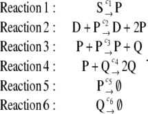
These reactions convert substrate molecules S into proteins Q. An intermediate protein P is first produced by Reaction 1 and, subsequently, by Reaction 2 via transcription and translation in which P acts as a transcription factor to promote its own synthesis from a DNA template D. P is then transformed into Q via the intermolecular reactions 3 and 4, with P and Q, respectively. Finally, Reactions 5 and 6 model degradation of P and Q. Due to Reactions 2 and 3, we refer to this system as quadratic autocatalator with positive feedback, since Reaction 3 is autocatalytic with quadratic concentration dependence (see also (24)) and Reaction 2 applies (positive) feedback on the synthesis of P. The resulting system is similar to a reaction cascade considered in Kaufman et al. (25), which involves the autophosphorylation of protein tyrosine kinase activity in T cell stimulation, obtained by ignoring all dephosphorylation reactions. This simplification leads to a biologically relevant example, which allows us to analytically demonstrate that intrinsic stochastic fluctuations may appreciably affect, both qualitatively and quantitatively, the stationary behavior of a biochemical reaction system. We could use more complicated reaction schemes (e.g., schemes that involve phosphorylation/dephosphorylation, transcription, translation, etc.), but it would not be possible to proceed analytically.

Quantitative stationary behavior

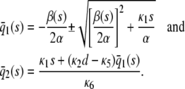
The steady-state concentrations of P and of Q, predicted by the SCKEs associated with the quadratic autocatalator with feedback are given by (see Appendix C for details)

(13)

(14)

where

(15)

provided that α > 0 and (see also the first row of Table 1). In these equations, s = S/AV and d = D/AV, where S, D are the numbers of S and D molecules, respectively. Moreover, is the sum of the mesoscopic fluxes of the third and fourth reactions at steady state, which depends on s, and the κ-values are the reaction rate constants, given by Eq. 42. We use the notation , , and to explicitly denote that the stationary quantities , , and depend on the input substrate concentration s. By setting in Eq. 13 (i.e., by ignoring the mesoscopic fluxes), we obtain the steady-state concentrations predicted by the CKEs (see Table 2).

TABLE 1.

Stationary concentrations of P, predicted by the SCKEs, in the quadratic autocatalator with feedback

α > 0	β(s) ≥ 0	β(s) < 0
		or
	No steady-state concentration

TABLE 2.

Stationary concentrations of P, predicted by the CKEs, in the quadratic autocatalator with feedback

α > 0	β(s) ≥ 0	β(s) < 0
s = 0		or
s > 0

According to Eq. 14, when κ₅ = κ₂d, the steady-state concentration of Q predicted by the SCKEs will be identical to the one predicted by the CKEs; this concentration is given by κ₁s/κ₆. However, this may not be true for the steady-state concentration of P, since this concentration depends on , according to Eq. 13. If , then Eqs. 13 and 14 imply that (this is also true when κ₅ ≠ κ₂d; see Appendix C), in which case, both models will asymptotically (as s →∞) reach the same steady-state concentration for P as well. However, for finite input substrate concentrations, we may not be able to ignore the steady-state mesoscopic forcing term , in which case the steady-state concentration of P predicted by the SCKEs will be different than the one predicted by the CKEs, with the difference being controlled by the sign and magnitude of . 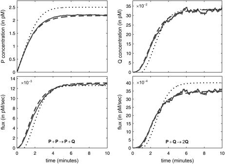This is illustrated in Fig. 2, which depicts the concentration dynamics of P and Q and the flux dynamics of the third and fourth reactions predicted by the SCKEs (solid lines), estimated by Monte Carlo simulation using the Gillespie algorithm, and the CKEs (dotted lines), obtained numerically. In this case, the steady-state P concentration predicted by the CKEs is larger than the one predicted by the SCKEs, since . Note the quantitative differences between the transient mean concentration dynamics and fluxes. As a matter of fact, the CKEs wrongly predict that the mean concentration of Q will be zero during the first minute, whereas the SCKEs predict a gradual increase in the mean concentration of Q from 0 pM to ∼0.033 pM.

FIGURE 2.

Protein accumulation in the quadratic autocatalator, given by Eq. 12, for the case when κ₅ = κ₂d, initialized with 10 molecules S (concentration of 8.30 pM), two molecules D (the number of DNA copies of a particular gene per eukaryotic cell), and zero molecules P and Q, predicted by the SCKEs (solid lines) and CKEs (dotted lines). The dynamics obtained by the SCKEs have been computed by Monte Carlo simulation using the Gillespie algorithm, whereas the dynamics obtained by the CKEs have been computed numerically. The flux dynamics of the third and fourth reactions are depicted as well. Parameters used are c₁ = 0.002 s⁻¹, c₂ = 0.001 s⁻¹, c₃ = 0.005 s⁻¹, c₄ = 0.004 s⁻¹, c₅ = 0.002 s⁻¹, c₆ = 0.05 s⁻¹, V = 2 pL, and K = 10,000 cells. Although the steady-state concentration of Q predicted by the CKEs is theoretically identical to the one predicted by the SCKEs, this is not true for the concentration of P. The dashed lines indicate the mean concentration and flux dynamics predicted by the second-order SCKEs discussed in this article.

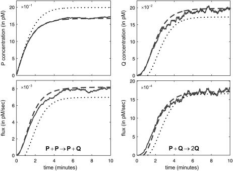
Similar remarks apply when κ₅ ≠ κ₂d. However, the steady-state concentrations of both P and Q depend now on (the concentration of Q depends on through the concentration of P; recall Eq. 14) and the CKEs may not provide good approximations at finite input substrate concentrations. We illustrate this case in Fig. 3.

FIGURE 3.

Protein accumulation and flux dynamics in the quadratic autocatalator, given by Eq. 12, for the case when κ₅ > κ₂d. The parameters used are the same as in Fig. 2, but now c₅ = 0.006 s⁻¹. In this case, the steady-state concentrations of P and Q predicted by the CKEs (dotted lines) are both different than the actual steady-state concentrations predicted by the SCKEs (solid lines). The dashed lines indicate the mean concentration and flux dynamics predicted by the second-order SCKEs discussed in this article.

Our previous investigation shows that intrinsic stochastic fluctuations may produce appreciable quantitative differences between the stationary behavior of a biochemical reaction system predicted by classical chemical kinetics and the stationary behavior predicted by stochastic chemical kinetics. These differences are caused by nonzero mesoscopic forcing terms at steady state, which may influence stationary molecular concentrations and appreciably affect their values.

The stationary behavior of biochemical activity may affect cells in a biologically significant way. For example, it has been suggested that concentrations of regulatory proteins synthesized at steady state may be responsible for a cell's unique characteristics (phenotype) (26). As a consequence, the previous analytical and numerical investigations show that intrinsic stochastic fluctuations may quantitatively affect the epigenetic properties of cell regulation in a manner not accounted for by classical chemical kinetics. In addition, we show in the following that nonzero stationary mesoscopic forcing terms may influence the steady-state properties of a biochemical reaction system in a qualitative way, thus demonstrating the fact that intrinsic stochastic fluctuations may play a significant role in influencing cellular function.

Qualitative stationary behavior

In the quadratic autocatalator with positive feedback, the stationary concentration of P predicted by the SCKEs depends on the signs of parameters α and β(s), given by Eq. 15, and the value of the input flux κ₁s as compared to the value of the steady-state mesoscopic forcing term . The resulting concentrations are summarized in Table 1 for α > 0 (similar results hold for α < 0). In particular, if , the system has a unique stable stationary P concentration , given by Eq. 13, regardless of the value of β(s). The situation, however, is different when . If and β(s) ≥ 0, the system relaxes to a zero P concentration at steady state, whereas, if and β(s) ≥ 0, the system has no stationary P concentration. However, if and β(s) < 0, the system has two stationary P concentrations and , given by

and

Note that , with the two concentrations being equal when the input substrate concentration is set to , where satisfies = .

On the other hand, although the stationary concentration of P predicted by the CKEs still depends on the signs of parameters α and β(s), this concentration does not depend on the input flux values κ₁s but only on whether or not the input substrate concentration is zero. The resulting concentrations are summarized in Table 2, for α > 0. When s = 0 and β(0) ≥ 0, the CKEs predict zero stationary P concentration, whereas, when s = 0 and β(0) < 0, the CKEs predict two stationary P concentrations, and , with the former being stable and the latter unstable. However, when s > 0, the CKEs predict a unique steady-state P concentration, regardless of the value of s and β(s), which is the same as the concentration predicted by the SCKEs, given by Eq. 13 with .

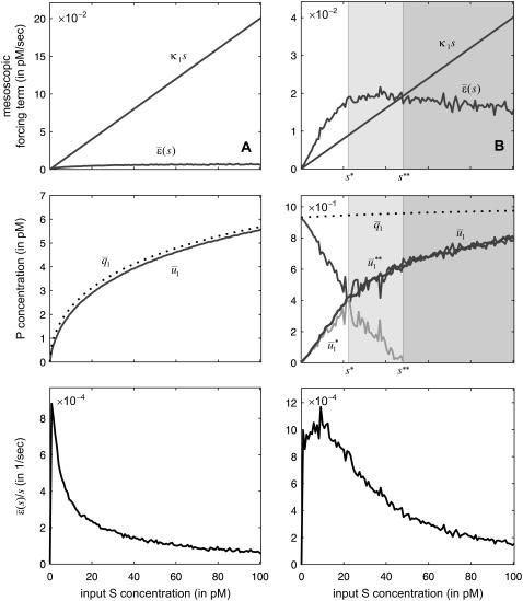
To illustrate the previous analytical results and demonstrate their biological significance, we depict in Fig. 4 the stationary concentration of P as a function of the input substrate concentration s, predicted by the SCKEs (solid lines), estimated by Monte Carlo simulation using the Gillespie algorithm, and by the CKEs (dotted lines), obtained analytically. In Fig. 4 A, , for every s > 0, in which case, the steady-state response curve predicted by the SCKEs will be given by . The response curve , predicted by the CKEs, is similar to the one predicted by the SCKEs, with , since . The situation, however, is very different in Fig. 4 B, in which , for , and , for , where is the input substrate concentration that satisfies . In this case, the steady-state response curve predicted by the SCKEs is obtained by stitching together three stable stationary P concentrations, namely, , for 0 ≤ s ≤ ≃ 22.5 pM, , for ≤ s ≤ , and , for s ≥ . Note that the slope of is larger than the slope of , whereas, the slope of tends to zero as s →∞. As a consequence, and similarly to the behavior shown in Fig. 4 A, the system experiences appreciable protein amplification at low input substrate concentrations (i.e., for s ≤ ; see the open region in Fig. 4 B), a moderate amplification at intermediate input concentrations (i.e., for —see the light shaded region in Fig. 4 B), and diminishing amplification at high input concentrations (i.e., for ; see the dark shaded region in Fig. 4 B). This behavior is essential to guarantee that, besides its normal operational range, the system responds quickly to low input substrate concentrations (high amplification) but very slowly to high concentrations (saturation). Note that the steady-state response curve predicted by the CKEs increases abruptly from 0 pM to ∼0.95 pM at s = 0, thus failing to capture the previous “multistage” amplification property. However, since , we have that , and the two response curves predicted by the CKEs and the SCKEs will eventually coincide for a sufficiently large input substrate concentration.

FIGURE 4.

The input flux k₁s versus the stationary mesoscopic forcing term , the stationary concentration of P as a function of s, predicted by the SCKEs (solid lines) and CKEs (dotted lines), and the ratio associated with the quadratic autocatalator, given by Eq. 12. The steady-state values obtained by the SCKEs have been computed by Monte Carlo simulation using the Gillespie algorithm, whereas the values obtained by the CKEs have been computed analytically. The system is initialized with two molecules D (the number of DNA copies of a particular gene per eukaryotic cell), and zero molecules P and Q. Parameters used are (A) c₁ = 0.002 s⁻¹, c₂ = 0.0005 s⁻¹, c₃ = 0.005 s⁻¹, c₄ = 0.004 s⁻¹, c₅ = 0.004 s⁻¹, c₆ = 0.05 s⁻¹, and (B) c₁ = 0.0004 s⁻¹, c₂ = 0.02 s⁻¹, c₃ = 0.05 s⁻¹, c₄ = 0.04 s⁻¹, c₅ = 0.01 s⁻¹, and c₆ = 0.05 s⁻¹. Moreover, V = 2 pL and K = 8000 cells. The heavy bold line in the middle figure depicts the steady-state response curve of P, calculated by Monte Carlo simulation using the Gillespie algorithm.

As a consequence of the previous investigations, intrinsic stochastic fluctuations may appreciably affect the qualitative properties of a biochemical reaction system at steady state. This can be analytically explained by the presence of nonzero mesoscopic forcing terms, which are responsible for introducing novel modes of behavior not accounted for by classical chemical kinetics. The significance of these modes should not be underestimated, since they may introduce behavior at low molecular concentrations that is essential for proper biological function.

Second-order SCKE approximation

It is unfortunate that we cannot compute the mesoscopic forcing term ɛ(t) analytically. As a consequence, we cannot use standard numerical techniques to solve the SCKEs 9 (or Eqs. 5–8). Instead, we resort to Monte Carlo simulations using the Gillespie algorithm. However, to obtain accurate Monte Carlo estimates of mean concentration dynamics and fluxes, we need to uniformly sample the system state for a large number of DA trajectories. (Note that the variance of a Monte Carlo estimator with uniform sampling is ∼1/K, where K is the number of samples used.) This approach is computationally intensive and especially burdensome when the biochemical reaction system is large and highly reactive.

To circumvent the computational expense of Monte Carlo simulation, we can approximate the SCKEs 5–8 by a system of first-order ordinary differential equations, which we can solve efficiently by the same numerical techniques we use to solve the CKEs. As a matter of fact, we can approximate the mean molecular concentrations u(t) by concentrations that satisfy the system of differential equations (see Appendix D) as

(16)

with

(17)

where the m^th elements of and are given by

(18)

(19)

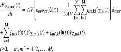
In Eq. 19, the terms approximate the DA covariances v_Z,mm′(t) and satisfy the system of first-order ordinary differential equations,

(20)

where δ_mm′ is the Krönecker delta given by Eq. 31, and ζ_m,k is the first-order partial derivative of the propensity function of the m^th reaction with respect to z_k, given by

For reasons explained in Appendix D, we refer to Eqs. 16–20 as second-order SCKEs.

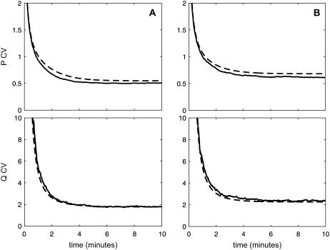
We illustrate the quality of approximation obtained by the second-order SCKEs in Figs. 2 and 3, for the case of the quadratic autocatalator with feedback. For this example, the second-order SCKEs provide excellent approximations (dashed lines) of the mean concentration dynamics predicted by the CME (solid lines), which are clearly better than the approximations obtained with the CKEs (dotted lines). We also show in Fig. 5 that, by using the second-order SCKEs, we can obtain very good approximations of the dynamic evolutions of the coefficients of variation (CVs) associated with the intrinsic stochastic fluctuations in P and Q concentrations. (The CVs provide a measure of the relative dispersion, i.e., size, of stochastic fluctuations in the concentration of a molecular species from the mean value; see Appendix D.) It is clear that calculation of CVs is not possible with the CKEs. The reader may also refer to Fig. 2 and Fig. 6 in Goutsias (23) for results obtained with a more complex biological system, which includes transcription, translation, protein dimerization, and molecular degradation. Therefore, in addition to satisfactorily approximating the mean concentration dynamics, we may use the second-order SCKEs to characterize intrinsic fluctuations in a stochastic biochemical reaction system by approximating CV dynamics.

FIGURE 5.

CV dynamics in the quadratic autocatalator, given by Eq. 12, associated with intrinsic stochastic fluctuations in the concentrations of P and Q, for the case when κ₅ = κ₂d, in panel A, and κ₅ > κ₂d, in panel B, predicted by the exact SCKEs (solid lines) and second-order SCKEs (dashed lines). The dynamics obtained by the exact SCKEs have been computed by Monte Carlo simulation using the Gillespie algorithm, whereas the dynamics obtained by the second-order SCKEs have been computed numerically. The parameters used are the same as in Figs. 2 and 3.

FIGURE 6.

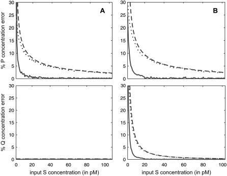
Absolute relative errors in the steady-state concentrations of P and Q associated with the quadratic autocatalator, given by Eq. 12, as a function of the input substrate concentration. (Solid lines) Second-order SCKEs with respect to the exact SCKEs; (dotted lines) CKEs with respect to the exact SCKEs; and (dashed lines) CKEs with respect to the second-order SCKEs. The steady-state values obtained by the exact and second-order SCKEs have been respectively computed by Monte Carlo simulation using the Gillespie algorithm and numerically, whereas the values obtained by the CKEs have been computed analytically from Eq. 44. The system is initialized with two molecules D (the number of DNA copies of a particular gene per eukaryotic cell), and zero molecules P and Q. Parameters used are c₁ = 0.002 s⁻¹, c₂ = 0.001 s⁻¹, c₃ = 0.005 s⁻¹, c₄ = 0.004 s⁻¹, c₆ = 0.05 s⁻¹, V = 2 pL, and K = 8000 cells. Moreover, c₅ = 0.002 s⁻¹ in panel A, and c₅ = 0.006 s⁻¹ in panel B.

Extensive simulations reveal that the quadratic autocatalator can be approximated very well by the second-order SCKEs for a wide range of parameter values and molecular concentrations (data not shown). One notable exception is at very low substrate concentrations s, in which case the biochemical reaction system will contain a very small number of molecules. We illustrate this in Fig. 6, which depicts the absolute relative errors in the steady-state mean concentrations of P and Q predicted by the second-order SCKEs with respect to the exact SCKEs (solid lines), by the CKEs with respect to the exact SCKEs (dotted lines), and by the CKEs with respect to second-order SCKEs (dashed lines), for the case when κ₅ = κ₂d, in Fig. 6 A, and κ₅ > κ₂d, in Fig. 6 B. Clearly, the second-order SCKEs provide consistently good and better approximations than the CKEs. As expected, when κ₅ = κ₂d, the errors in approximating the steady-state Q concentration are zero. Moreover, the errors in the concentrations of P and Q predicted by the two models gradually diminish for large input substrate concentrations. Note however that the accuracy of the second-order SCKEs decreases at very small input substrate concentrations.

A good match between the predictions obtained by the second-order SCKEs and the ones obtained by the exact SCKEs indicates that the mean and covariances provide a sufficient description of intrinsic stochastic fluctuations, in which case, the molecular distributions will approximately follow a Gaussian distribution. However, the observation that, at very small input substrate concentrations, the second-order SCKEs may not sufficiently approximate the dynamics obtained by the exact SCKEs strongly suggests that higher-order (≥3) central moments may play a significant role in determining these dynamics. In this case, the underlying reactions will be subject to appreciable higher-order statistical interactions and the underlying probability distributions will not be Gaussian. Recent findings suggest that molecular distributions are often non-Gaussian and that such distributions may play an important role in cellular regulation (27,28). In those cases, it will be necessary to derive higher-order SCKE approximations, by including higher-order moments in the formulation (see our discussion in Appendix D).

CONCLUSIONS

In this article, by adopting a general framework for modeling the macroscopic behavior of a biochemical reaction system consisting of elementary irreversible reactions, we have shown that a classical chemical kinetics approach to modeling biochemical reaction systems may not be appropriate. The flux of each reaction is decomposed into two terms, a macroscopic term that accounts for the effects of mean molecular concentrations on the macroscopic behavior of the system and a mesoscopic term that accounts for the effects of pairwise correlations among reactions. Based on this decomposition, we may characterize a biochemical reaction system by a system of exact first-order ordinary differential equations, the SCKEs, which provide a straightforward extension to the classical CKEs. The SCKEs require use of mesoscopic forcing terms, obtained by linearly transforming the mesoscopic fluxes through the stoichiometry matrix, whose calculation requires computationally expensive Monte Carlo simulations or evaluation of correlation dynamics among pairs, triplets, quadruplets, and larger groups of biochemical reactions.

To avoid such calculations, we have focused on a second-order approximation to the SCKEs, which includes only first- and second-order reaction statistics (i.e., means and pairwise correlations). These equations can be solved by standard numerical procedures and may lead to versatile tools for the analysis of biochemical reaction systems, similar to the ones used in classical chemical kinetics. Notably, a first-order approximation to the SCKEs produces the equations of classical chemical kinetics.

Our analysis indicates that pairwise correlation effects may lead, through mesoscopic forcing terms, to a dynamic behavior not accounted for by classical chemical kinetics. Numerical analysis of a quadratic autocatalator with positive feedback shows that the proposed second-order approximation faithfully reproduces system behavior, for a wide range of molecular concentrations and kinetic parameters. The success of this approximation demonstrates that the second-order SCKEs may provide substantial simplification in describing and analyzing stochastic biochemical reaction systems. Moreover, it suggests that pairwise statistical interactions among reactions may be sufficient for determining biological function and supports the use of multivariate Gaussian distributions for modeling biochemical reactions. However, this may not be true at very low molecular concentrations in which case higher-order approximations may be necessary. The need to include higher-order moments in the approximation highlights the importance of higher-order interactions among biochemical reactions and the inappropriateness of Gaussian modeling at very low molecular concentrations.

APPENDIX A: STOCHASTIC CHEMICAL KINETICS

Since biochemical reactions occur by random collisions of reactant molecules, the number of molecules of a particular species present in the system at time t may fluctuate randomly. It is therefore appropriate to characterize the state of a biochemical reaction system at time t by an N × 1 random vector X(t) whose n^th element X_n(t) is the number of molecules of the n^th species present in the system at time t. In addition, we may use the degree of advancement (DA) Z_m(t) to describe the (random) progress of the m^th reaction during the time interval [0, t), where Z_m(t) = z ≥ 0 means that the m^th reaction has occurred z times during the time interval [0, t) (29). Note that, due to conservation of mass, we can uniquely determine X(t) from the M × 1 random vector Z(t) with elements Z_m(t), m = 1, 2, …, M, since

(21)

Recall that our objective is to model the dynamic evolutions of molecular concentrations in a tissue containing a large population of cells by the N × 1 vector u(t) given by Eq. 1. By taking expectations on both sides of Eq. 21 and by dividing with AV, we obtain

(22)

where u(0) = x(0)/AV and μ_Z(t) = E[Z(t)]. If we assume that the mean DA μ_Z(t) is differentiable with respect to t (see below why this is true), then, by differentiating both sides of Eq. 22, we obtain Eq. 5. The average reaction rate (flux) ν_m(t) of the m^th reaction is given by

(23)

where χ_m(t) is the average extent of the m^th reaction defined as the mean DA of the reaction divided by the Avogadro number; i.e.,

(24)

Computation of ν_m(t) requires calculation of the derivative of the mean DA μ_Z,m(t) with respect to t. We show how to calculate this derivative in the following.

We denote by ϕ_m(x) the number of all possible distinct combinations of the reactant molecules of the m^th reaction channel when the system is at state x, given by (compare with Eq. 4)

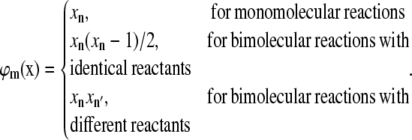(25)

We also denote by c_m the specific probability rate constant of the m^th reaction (i.e., the probability per unit time that a randomly chosen combination of reactant molecules will react through the m^th reaction channel). Then, given that the biochemical reaction system is at state X(t) = x at time t, the probability that one m^th reaction will occur during the time interval [t, t + dt) is π_m(x)dt + o(dt), for a sufficiently small dt, where o(dt) is defined so that o(dt)/dt → 0, as dt → 0, and

(26)

is the propensity function of the m^th reaction channel (30,31). Moreover, the probability that more than one reaction will occur during [t, t + dt) is o(dt).

If P_Z(z;t) = Pr (Z(t) = z) is the probability that the DA vector Z(t) takes value z at time t, then (23,32,33)

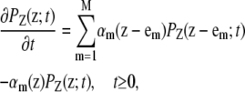(27)

where e_m is the m^th column of the M × M identity matrix, and

(28)

This chemical master equation (CME) describes the dynamic evolution of the joint probability mass function of the DA process Z(t). As a consequence, we can show that the means μ_Z,m(t) and covariances v_Z,mm′(t) of the DA process Z(t) satisfy the system of first-order ordinary differential equations (23),

(29)

(30)

for t ≥ 0, where δ_mm′ is the Krönecker delta, given by

(31)

Note that the derivatives dμ_Z,m(t)/dt and dv_Z,mm′(t)/dt always exist at finite times, regardless of the number of molecules present in the system, since the CME (Eq. 27) is valid only when the joint probability mass function P_Z(z;t) is a continuous function of t, which in turn implies that the means μ_Z,m(t) and covariances v_Z,mm′(t) are continuous functions of t as well.

If we expand the propensity function α_m(z) by a Taylor series about the mean vector μ_z(t), we have

(32)

where ζ_m and denote the gradient vector (of the first-order partial derivatives with respect to z) and the Hessian matrix (of the second-order partial derivatives with respect to z) of α_m(z), respectively, and T denotes vector (matrix) transposition. From Eqs. 25, 26, and 28, note that the propensity function α_m is at most a quadratic function of the DAs. Therefore, its derivatives of order >2 are zero and Eq. 32 is exact. Moreover, the Hessian does not depend on z. By taking expectations on both sides of Eq. 32 and by using Eq. 29, we obtain

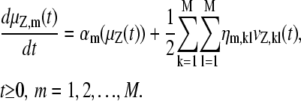(33)

In Eq. 33, η_m,kl is the (k, l) element of the Hessian matrix (i.e., the second-order partial derivative of the propensity function π_m(x) with respect to the DAs of the k^th and l^th reactions), given by

where ψ_m is given by Eq. 4 and

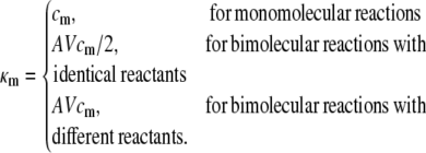(34)

Equation 34 relates the specific probability rate constants c with the reaction rate constants κ. Equations 6–8 are now obtained from Eqs. 4, 23–26, 28, 33, and 34.

APPENDIX B: UNIDIRECTIONAL DIMERIZATION

Let us consider the unidirectional dimerization reaction in Eq. 11. We denote its DA by Z₁(t) and use random variables X_n(t), n = 1, 2, 3, to characterize its state at time t ≥ 0, where each variable denotes the number of molecules of a reactant or product species, as identified by the following assignment:

Note that the stoichiometry matrix is given by

(35)

whereas, the propensity function is given by π₁(x₁, x₂, x₃) = c₁x₁x₂. If we initialize the reaction with x₁(0) = S molecules P, x₂(0) = S molecules Q, and x₃(0) = 0 molecules P·Q, then, from Eq. 21 and Eq. 35, we have that

(36)

Moreover, Eq. 28 implies that α₁(z₁) = c₁(S – z₁)².

Since the reaction is bimolecular with different reactants, ψ₁(u₁, u₂, u₃) = u₁u₂ (see Eq. 4). Moreover, from Eqs. 1 and 36, we have

where s = S/AV is the concentration of initial P or Q molecules. In this case, Eq. 9 implies the following SCKE for the dimer concentration u₃(t),

where the mesoscopic forcing term ɛ₃(t) is given by

and κ₁ = AVc₁, with initial conditions u₃(0) = ɛ₃(0) = 0. Moreover, Eq. 6 implies the following expression for the flux:

(37)

Finally, we can verify that the concentration q₃(t) and flux ρ₁(t) predicted by the CKE (obtained by setting ɛ₃(t) = 0, for every t ≥ 0), are given by

(38)

APPENDIX C: QUADRATIC AUTOCATALATOR

Let us now consider the six reactions in Eq. 12. We use variables X₁(t) and X₂(t) to characterize the molecular state of the system at time t ≥ 0, where each variable is identified by the following assignment:

In this case, the stoichiometry matrix is given by

(39)

whereas, the propensity functions are given by

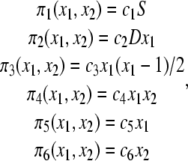with S and D being the number of S and D molecules, respectively, which we assume to be fixed. Note also that

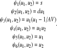(40)

Here, s = S/AV and d = D/AV. We initialize the reactions by setting X₁(0) = X₂(0) = 0. Then, from Eqs. 21 and 39, we have

Equations 9, 39, and 40 lead to the following SCKEs for characterizing the quadratic autocatalator with feedback,

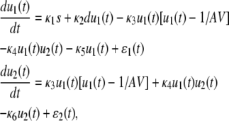(41)

for t ≥ 0, where

and (recall Eq. 34)

(42)

Note that θ₁(t) = θ₂(t) = θ₅(t) = θ₆(t) = 0, since the corresponding propensity functions are linear in z (reactions 1, 2, 5, and 6 are monomolecular) and their Hessian matrices are thus zero. The corresponding CKEs are obtained from Eq. 41 by setting ɛ₁(t) = ɛ₂(t) = 0, for every t ≥ 0.

If we set the right-hand sides of Eq. 41 (nullclines) equal to zero, we obtain the stationary solutions,

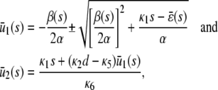(43)

with α and β given by Eq. 15, where , , and . Since only nonnegative solutions are relevant, the system will relax at steady state to molecular concentrations that depend on the signs of α, β, and on the value of the input flux κ₁s as compared to the value of the steady-state mesoscopic forcing term . We show this in Table 1, where we summarize the steady-state concentrations of P predicted by the SCKEs, which we obtain from Eq. 43 by assuming that α > 0 (we can obtain similar results for the case when α < 0). The corresponding steady-state concentrations of Q are obtained from the second Eq. 43, provided that . Note that, by setting in Eq. 43, we obtain the following stationary solutions of the CKEs:

(44)

For α > 0, the steady-state P concentrations predicted by the CKEs are summarized in Table 2.

Finally, if we make the reasonable assumption that, for every input substrate concentration, the steady-state mesoscopic forcing term is bounded, then

(45)

which implies that

Indeed, from Eq. 45 and for a sufficiently large s, we have that . Then,

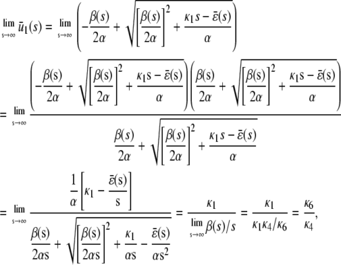since, from Eq. 15, . This implies that, in the limit of s→∞, the steady-state P concentration will not depend on . Therefore, for a sufficiently large input substrate concentration, the steady-state P and Q concentrations predicted by the CKEs will be approximately equal to the ones predicted by the SCKEs.

APPENDIX D: SCKE APPROXIMATIONS

To approximate the SCKEs 5–8, we should note that the behavior of a biochemical reaction system depends on the third-order central moments of the DA process Z(t). This dependence comes from the second and third terms on the right-hand side of Eq. 30, due to the second-order term in the Taylor series expansion of the propensity function, given by Eq. 32. Including these moments in the formulation requires an additional set of differential equations, which depend on fourth-order central moments, and so on. These nested dependencies rule out the possibility of determining the exact covariance values by solving the system of Eqs. 29 and 30.

To address this problem, we may employ a method of moment closure. For instance, it might be possible to find an expression for a higher-order moment in terms of lower-order moments, which would then make the system exactly solvable. However, we adopt a much simpler approach here, by setting the third-order central moments equal to zero (see also ((16,34)). These moments represent higher-order statistical dependencies among reaction channels due to bimolecular reactions. Note that higher-order statistical dependencies might become unimportant at some level. Since we do not know a priori when this might happen, we may assume that the third-order central moments have negligible effect on the DA means and covariances and subsequently check the resulting covariance approximations against the ones obtained by Monte Carlo estimation. If the results are not satisfactory, then we have to include higher-order (≥ 3) moments in the formulation. Note however that, although the task of including higher-order moments is straightforward, it will increase the number of differential equations in the approximation.

To derive our approximation, we expand each propensity function by a Taylor series about the mean DA vector μ_z(t) (see Eq. 32), we use this expansion in Eqs. 29 and 30, and set the third-order central moments of the DA process Z(t) equal to zero. As a consequence of these steps, we obtain the system of differential equations, Eqs. 16–20, which allow us to approximate the mean molecular concentrations u(t) by concentrations . Equations 16–20 provide a second-order approximation to the SCKEs, since we derive them by including only the first- and second-order moments of the DA process (i.e., the DA means and covariances). In this sense, the classical CKEs provide a first-order approximation to the SCKEs, since we can derive them by following the same steps but by including only the first-order DA moments (i.e., the DA means). In most cases of interest, we expect that the second-order SCKEs will provide sufficiently good approximations of the mean concentration dynamics, which will be more accurate than the approximations obtained by the CKEs.

In sharp contrast to the CKEs, we can use the second-order SCKEs to approximate the CVs associated with a biochemical reaction system. (The CV associated with the n^th molecular species at time t is the ratio of the square-root of the n^th diagonal element of the covariance matrix C_x(t) of the molecular population process X(t), divided by the corresponding mean.) Moreover, we can use the second-order SCKEs to approximate the correlation dynamics between the concentrations of two molecular species, quantified by the correlation coefficient. To do so, we can use the fact that the covariance matrix C_x(t) is related to the covariance matrix C_z(t) of the DA process Z(t) by means of , since (recall Eq. 21), and approximate C_x(t) by , where is a matrix with elements .

An alternative way to approximate the concentration dynamics is to use Eqs. 16–18 and recognize (by virtue of Eq. 19 and the fact that ) that

(46)

where h_m,kl is the second-order partial derivative of the propensity function of the m^th reaction with respect to x_k and x_l. The terms in Eq. 46 approximate the covariances of the molecular population process X(t) and can be shown to satisfy the system of first-order ordinary differential equations

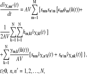where γ_m,k is the first-order partial derivative of the propensity function of the m^th reaction with respect to x_k, given by

When the number N of molecular species is smaller than the number M of reactions, this approach will be computationally more advantageous than calculating the DA covariances, since the number of population covariances, which is given by N(N + 1)/2, will be smaller than the number of DA covariances, which is given by M(M + 1)/2. However, we have briefly discussed in Goutsias (23) that characterizing a stochastic biochemical reaction system by means of the DA process Z(t) may be more advantageous in certain circumstances than characterizing the system by means of the molecular population process X(t). Because our developments in this article are based on the DA process Z(t), we use Eqs. 16–20 in our numerical investigations.

We can also derive the second-order SCKEs 16–20 by assuming that the most important influence on the firing rate of a given reaction in a stochastic biochemical reaction system is exerted by the mean propensity function of that reaction through a Poisson process and use an appropriately chosen zero mean additive correction term to compensate for statistical variations not accounted for by the Poisson process. This leads to a mean-field approximation of the system whose state Z(t) approximately follows a normal Gibbs distribution at temperature 2/k_B, with energy function , where k_B is the Boltzmann constant and the elements of satisfy Eq. 33 with v_{Z, kl}(t) being replaced by . The reader is referred to Goutsias (23) for details.

The SCKE approximation method employed in this article is one of several alternative strategies for approximating stochastic biochemical reaction systems (e.g., see (23)). A frequently used technique is the linear noise approximation method (29,35). This method is obtained from a Langevin approximation of the stochastic biochemical reaction system by 1), linearizing the propensity functions about the mean DA values, and 2), taking the limit of the resulting linear Fokker-Planck equation as the system volume tends to infinity (e.g., see (23)). Linearization of the propensity functions implies that their second-order partial derivatives with respect to the DAs will be zero. In turn, this implies that the mesoscopic fluxes and, therefore, the mesoscopic forcing terms will also be zero. Hence, the linear noise approximation method leads to the same system of differential equations for the mean concentration dynamics as the one obtained by classical chemical kinetics. As a consequence, the linear noise approximation method suffers from the same drawbacks as classical chemical kinetics and should be used with caution when investigating the effects of intrinsic stochastic fluctuations on biological function at low molecular concentrations.

References

- 1.Heinrich, R., and S. Schuster. 1996. The Regulation of Cellular Systems. Chapman and Hall, New York.
- 2.McAdams, H. H., and A. Arkin. 1999. It's a noisy business! Genetic regulation at the nanomolar scale. Trends Genet. 15:65–69. [DOI] [PubMed] [Google Scholar]
- 3.Rao, C. V., D. M. Wolf, and A. P. Arkin. 2002. Control, exploitation and tolerance of intracellular noise. Nature. 420:231–237. [DOI] [PubMed] [Google Scholar]
- 4.Kaern, M., T. C. Elston, W. J. Blake, and J. J. Collins. 2005. Stochasticity in gene expression: from theories to phenotypes. Nat. Rev. Genet. 6:451–464. [DOI] [PubMed] [Google Scholar]
- 5.McAdams, H. H., and A. Arkin. 1997. Stochastic mechanisms in gene expression. Proc. Natl. Acad. Sci. USA. 94:814–819. [DOI] [PMC free article] [PubMed] [Google Scholar]
- 6.Arkin, A., J. Ross, and H. H. McAdams. 1998. Stochastic kinetic analysis of developmental pathway bifurcation in phage λ-infected Escherichia coli cells. Genetics. 149:1633–1648. [DOI] [PMC free article] [PubMed] [Google Scholar]
- 7.Ozbudak, E. M., M. Thattai, I. Kurtser, A. D. Grossman, and A. van Oudenaarden. 2002. Regulation of noise in the expression of a single gene. Nat. Genet. 31:69–73. [DOI] [PubMed] [Google Scholar]
- 8.Blake, W. J., M. Kaern, C. R. Cantor, and J. J. Collins. 2003. Noise in eukaryotic gene expression. Nature. 422:633–637. [DOI] [PubMed] [Google Scholar]
- 9.Ozbudak, E. M., M. Thattai, H. N. Lim, B. I. Shraiman, and A. van Oudenaarden. 2004. Multistability in the lactose utilization network of Escherichia coli. Nature. 427:737–740. [DOI] [PubMed] [Google Scholar]
- 10.Peixoto, A., M. Monteiro, B. Rocha, and H. Veiga-Fernandes. 2004. Quantification of multiple gene expression in individual cells. Genome Res. 14:1938–1947. [DOI] [PMC free article] [PubMed] [Google Scholar]
- 11.Shav-Tal, Y., R. H. Singer, and X. Darzacq. 2004. Imaging gene expression in single living cells. Nat. Rev. Mol. Cell Biol. 5:856–862. [DOI] [PMC free article] [PubMed] [Google Scholar]
- 12.Capodieci, P., M. Donovan, K. Buchinsky, Y. Jeffers, C. Cordon-Cardo, W. Gerald, J. Edelson, S. M. Shenoy, and R. H. Singer. 2005. Gene expression profiling in single cells within tissue. Nat. Methods. 2:663–665. [DOI] [PMC free article] [PubMed] [Google Scholar]
- 13.Bowtell, D. D. L. 1999. Options available—from start to finish—for obtaining expression data by microarray. Nat. Genet. 21:25–32. [DOI] [PubMed] [Google Scholar]
- 14.Lockhart, D. J., and E. A. Winzeler. 2000. Genomics, gene expression and DNA arrays. Nature. 405:827–836. [DOI] [PubMed] [Google Scholar]
- 15.McQuarrie, D. A., C. J. Jachimowski, and M. E. Russell. 1964. Kinetics of small systems. II. J. Chem. Phys. 40:2914–2921. [Google Scholar]
- 16.Thakur, A. K., A. Rescigno, and C. DeLisi. 1978. Stochastic theory of second-order chemical reactions. J. Phys. Chem. 82:552–558. [Google Scholar]
- 17.Leonard, D., and L. E. Reichl. 1990. Stochastic analysis of a driven chemical reaction. J. Chem. Phys. 92:6004–6010. [Google Scholar]
- 18.Zheng, Q., and J. Ross. 1991. Comparison of deterministic and stochastic kinetics for nonlinear systems. J. Chem. Phys. 94:3644–3648. [Google Scholar]
- 19.Savageau, M. A. 1976. Biochemical Systems Analysis: A Study of Function and Design in Molecular Biology. Addison-Wesley, Reading, MA.
- 20.Samoilov, M., S. Plyasunov, and A. P. Arkin. 2005. Stochastic amplification and signaling in enzymatic futile cycles through noise-induced bistability with oscillations. Proc. Natl. Acad. Sci. USA. 102:2310–2315. [DOI] [PMC free article] [PubMed] [Google Scholar]
- 21.Darvey, I. G., and P. J. Staff. 1966. Stochastic approach to first-order chemical reaction kinetics. J. Chem. Phys. 44:990–997. [Google Scholar]
- 22.Gillespie, D. T. 1977. Exact stochastic simulation of coupled chemical reactions. J. Phys. Chem. 81:2340–2361. [Google Scholar]
- 23.Goutsias, J. 2006. A hidden Markov model for transcriptional regulation in single cells. IEEE/ACM Trans. Comput. Biol. Bioinf. 3:57–71. [DOI] [PubMed] [Google Scholar]
- 24.Scott, S. K. 1991. Chemical Chaos. Oxford University Press, Oxford, UK.
- 25.Kaufman, M., F. Andris, and O. Leo. 1996. A model for antigen-induced T cell unresponsiveness based on autophosphorylative protein tyrosine kinase activity. Int. Immunol. 8:613–624. [DOI] [PubMed] [Google Scholar]
- 26.Alberts, B., A. Johnson, J. Lewis, M. Raff, K. Roberts, and P. Walter. 2002. Molecular Biology of the Cell, 4th Ed. Garland Publishing, New York.
- 27.Banerjee, B., S. Balasubramanian, G. Ananthakrishna, T. V. Ramakrishnan, and G. V. Shivashankar. 2004. Tracking operator state fluctuations in gene expression in single cells. Biophys. J. 86:3052–3059. [DOI] [PMC free article] [PubMed] [Google Scholar]
- 28.Krishna, S., B. Banerjee, T. V. Ramakrishnan, and G. V. Shivashankar. 2005. Stochastic simulations of the origins and implications of long-tailed distributions in gene expression. Proc. Natl. Acad. Sci. USA. 102:4771–4776. [DOI] [PMC free article] [PubMed] [Google Scholar]
- 29.van Kampen, N. G. 1992. Stochastic Processes in Physics and Chemistry. Elsevier, Amsterdam, The Netherlands.
- 30.Gillespie, D. T. 1992. A rigorous derivation of the chemical master equation. Physica A. 188:404–425. [Google Scholar]
- 31.Gillespie, D. T. 2000. The chemical Langevin equation. J. Chem. Phys. 113:297–306. [Google Scholar]
- 32.Haseltine, E. L., and J. B. Rawlings. 2002. Approximate simulation of coupled fast and slow reactions for stochastic chemical kinetics. J. Chem. Phys. 117:6959–6969. [Google Scholar]
- 33.Goutsias, J. 2005. Quasiequilibrium approximation of fast reaction kinetics in stochastic biochemical systems. J. Chem. Phys. 122:184102. [DOI] [PubMed] [Google Scholar]
- 34.Pirone, J. R., and T. C. Elston. 2004. Fluctuations in transcription factor binding can explain the graded and binary responses observed in inducible gene expression. J. Theor. Biol. 226:111–121. [DOI] [PubMed] [Google Scholar]
- 35.Elf, J., and M. Ehrenberg. 2003. Fast evaluation of fluctuations in biochemical networks with the linear noise approximation. Genome Res. 13:2475–2484. [DOI] [PMC free article] [PubMed] [Google Scholar]