

Abstract
Human visual performance is better below than above fixation along the vertical meridian – vertical meridian asymmetry (VMA). Here we used fMRI to investigate the neural correlates of the VMA. We presented stimuli of two possible sizes and spatial frequencies on the horizontal and vertical meridians and analyzed the fMRI data in subregions of early visual cortex (V1/V2) that corresponded retinotopically to the stimulus locations. Asymmetries in both the spatial extent and amplitude of the fMRI measurements correlated with the behavioral VMA. These results demonstrate that the VMA has a neural basis at the earliest stages of cortical visual processing, and imply that visual performance is limited by the pooled sensory responses of large populations of neurons in visual cortex.
Keywords: vision, vertical meridian, psychophysics, visual cortex, fMRI
Introduction
Human performance differs at different locations in the visual field. In addition to the performance reduction for visual locations in the periphery farther from the center of gaze (DeValois & DeValois, 1988; Duncan & Boynton, 2003), the lower visual field (below fixation) supports better performance than the upper visual field, even at the same eccentricity (Altpeter, Mackeben, & Trauzettel-Klosinski, 2000; Edgar & Smith, 1990; He, Cavanagh, & Intriligator, 1996; Levine & McAnany, 2005; Previc, 1990; Rubin, Nakayama, & Shapley, 1996). A series of studies report that this performance asymmetry in many tasks is restricted to the vertical meridian: performance is worse along the upper than the lower region of the vertical meridian, but shows no difference between upper and lower visual field for non-meridian locations (Cameron, Tai, & Carrasco, 2002; Carrasco, Giordano, & McElree, 2004; Carrasco, Talgar, & Cameron, 2001; Carrasco, Williams, & Yeshurun, 2002; Talgar & Carrasco, 2002). Hence, we have referred to this phenomenon as vertical meridian asymmetry (VMA). The VMA becomes more pronounced with increasing spatial frequency – it is barely present for low spatial-frequency Gabor stimuli, and gradually becomes more pronounced for intermediate and high frequencies (Cameron, Tai, & Carrasco, 2002; Carrasco, Talgar, & Cameron, 2001; Skrandies, 1987). This asymmetry has been observed in detection, discrimination and localization tasks, in which performance is based on contrast sensitivity (Cameron, Tai, & Carrasco, 2002; Carrasco, Talgar, & Cameron, 2001), acuity (Carrasco et al., 2002) and spatial resolution (Talgar & Carrasco, 2002). Here we investigated the neural correlate of the VMA.
Physiological studies with non-human primates have found differences in the upper versus lower field representations along the visual pathways. In the retina, the cone and ganglion cell densities are greater in lower than upper visual field (Perry & Cowey, 1985). Likewise, studies have shown that slightly more neural tissue is devoted to the lower than the upper visual field representations in LGN (Connolly & Van Essen, 1984), V1 (Tootell, Switkes, Silverman, & Hamilton, 1988; Van Essen, Newsome, & Maunsell, 1984), and MT (Maunsell & Van Essen, 1987). In humans, a larger MEG response amplitude for the lower than the upper visual field has been reported (Portin, Vanni, Virsu, & Hari, 1999). These differences, however, refer to visual hemi-fields, and are not specific to the vertical meridian. Indeed, no neurophysiological study has investigated the VMA.
We measured human brain activity evoked by visual stimulation at locations along the vertical meridian. We analyzed the fMRI data in subregions of early visual cortex (V1 and V2) that corresponded retinotopically to the cortical representations of the stimulus locations, and found asymmetries in cortical activity that correlated with behavioral performance. To ensure an unambiguous interpretation of our results, we manipulated the spatial frequency of the stimulus. This manipulation enabled us to rule out the possibility that only the hemodynamics differed between cortical locations without corresponding differences in the underlying neural activity evoked by the stimuli.
Methods
Observers
Five observers (3 women), all with normal or corrected-to-normal vision, participated in the experiment. All observers were experienced psychophysical observers. All observers but one (an author, TL) were naïve as to the purpose of the experiment. The experiments were performed following the safety guidelines for MRI research; informed consent was obtained, and the experimental protocol was approved by the Institutional Review Board at New York University. Each observer participated in several MRI scanning sessions on different days: One to obtain high-resolution anatomical images, one to measure retinotopic maps in visual cortex, and 1–3 sessions for the main experiment.
Visual Stimuli
Stimuli were presented on a rear-projection screen located in the scanner bore with an EIKI LC-XG100 LCD projector and a custom-made zoom lens. Observers viewed the screen via an angled mirror attached to the head coil, and a bite bar was used to stabilize their heads. Stimuli were generated using Matlab (MathWorks, Natick, MA) and the Psychophysics Toolbox software (Brainard, 1997; Pelli, 1997). The projector luminance was gamma-corrected and the background luminance was set to the middle of the range, at 320 cd/m2. The screen was refreshed at 60 Hz with a resolution of 1024 × 768 pixels.
Stimuli consisted of Gaussian-windowed, sinusoidal luminance patterns (Gabor stimuli, Figure 1), which were presented at full contrast and counter-phase flickered at 4 Hz. The spatial frequency of the Gabors was either 1.5 or 6 cycles/degree (cpd), and the size was either 2° or 4° in diameter (different sizes were used with the goal of distinguishing two alternate interpretations of the results, see Appendix). The Gabors were presented at four possible locations either on the vertical or horizontal meridians at an eccentricity of 6°. A small fixation point (0.2°) was presented in the center of the screen throughout the experiment.
Figure 1.

Schematic of stimuli and experimental protocol. The Gabor stimuli were low or high spatial frequency, and small or large size. Each of these 4 stimulus conditions were presented in separate scans. During each scan, the stimuli were presented in 12s blocks that alternated between the horizontal meridian (HM) and vertical meridian (VM).
Design and Task
Figure 1 depicts the four stimulus conditions: two spatial frequencies (low vs. high) and two sizes (small vs. large). The four conditions were presented in separate scans, in a random order for each observer. Each scanning session included 8 scans (two of each condition). Four observers completed two sessions on two different days, and one observer completed one session. During each scan, the stimuli were presented in 12 s blocks that alternated between the horizontal and vertical meridians. During each block two Gabors were presented simultaneously, either above and below or to the right and left of fixation. Each scan lasted 228 s and consisted of 9 cycles (24 s each) of alternation between the horizontal and vertical meridians, plus a 12 s fixation period at the end.
Observers performed a continuous detection/discrimination task throughout each scan. The Gabors were vertical most of the time. At random intervals, one of the two Gabors was tilted for 125 ms, either clockwise or counterclockwise (target events). Observers were instructed to detect these targets and report the direction of the tilt by pressing buttons on MR compatible button boxes held in both hands. The index and middle fingers of each hand indicated the target tilt (‘clockwise’ or ‘counterclockwise’) and location (left hand: left or upper location, right hand: right or lower location). The inter-target-interval was drawn from a uniform distribution from 1 to 5 s. The location of the target and the tilt direction were randomly determined for each target event. Observers were instructed to perform the task as accurately and quickly as possible while maintaining fixation.
To control task difficulty, the amount of target tilt was determined individually for each observer in a separate training session in the psychophysics lab using the method of constant stimuli. We varied the target tilt and measured psychometric functions for stimuli on the horizontal meridian in each of the four conditions (2 size × 2 spatial frequency). We then selected tilt values at ~ 70% accuracy, separately for each condition and each observer, for the fMRI experiment. Orientation thresholds were similar for the two sizes but thresholds were higher for the high (small size: 25±19, large size: 34±19, mean±std dev) than the low (small size: 9±2, large size: 9±3, mean±std dev) spatial frequency. In this continuous detection/discrimination task, responses made 1 s after the target offset were counted as false alarms. False alarms were rare (< 1 % for all observers) and did not vary as a function of condition or location (all p > .1). Hence, we used the hit rates to quantify performance accuracy. Note that tilt threshold was set for stimuli on the horizontal meridian for each of the 4 combinations of size and spatial frequency, allowing us to observe the asymmetry on the vertical meridian.
To determine whether the observed effects were specific to the vertical meridian, we repeated the experiment for stimuli located in the main diagonal locations (45° off the horizontal and vertical meridians). Each of two observers participated in an additional scanning session in which only the high spatial frequency (6 cpd), large stimulus (4°) condition was presented (6° eccentricity), alternating between the diagonals (upper-right and lower-left alternating with upper-left and lower-right). Orientation thresholds were 20° and 32° for the two observers, similar to that in the meridian experiment.
Localizer Scans and Retinotopic Mapping
In each scanning session, we also ran ‘localizer’ scans to independently define cortical regions responding to the stimuli. The localizer scans were identical to the scans in the main experiment with the following exceptions: The stimuli were composed of a compound grating of 1.5 and 6 cpd, and no orientation-change targets were presented. Observers were instructed to passively view the display while maintaining fixation. Two types of localizer scans were run, one for each stimulus size (2° and 4°). Each type of localizer was used to define regions-of-interest (ROIs) for the stimulus condition with the corresponding stimulus size. In each scanning session, two repetitions of each localizer were run (four localizer scans per session in total).
Early visual cortical areas were identified, separately for each observer, based on retinotopic mapping, following well-established procedures (DeYoe et al., 1996; Engel, Glover, & Wandell, 1997; Engel et al., 1994; Sereno et al., 1995). Borders between visual cortical areas were identified as phase reversals in a map of the polar angle representation of the visual field; the polar angle component of the retinotopic map was measured in a single scan with a rotating double-wedge checkerboard stimulus (Slotnick & Yantis, 2003), and the responses were visualized on an inflated surface representation of each observer’s brain.
Imaging Protocol
Magnetic resonance imaging was performed on a 3T Siemens Allegra head-only scanner (Erlangen, Germany) equipped with a volume transmit head-coil and a four-channel, phase-array, surface receive coil (NM-011 transmit head-coil and NMSC-021 receive-coil, NOVA Medical, Wakefield, MA, USA). Functional images were acquired using a T2*-weighted echo-planar imaging sequence (TR = 1.5 s, TE = 30 ms, flip angle = 75°, matrix size = 96 × 96, in-plane resolution = 2 × 2 mm, slice thickness = 2 mm, no gap). Twenty-two slices covering the occipital lobe and approximately perpendicular to the calcarine sulcus were acquired every 1.5 s. Images were reconstructed off-line from the raw k-space data using custom C and Matlab code (Fleysher, Fleysher, Heeger, & Inati, 2005). High-resolution anatomical images were acquired for each observer using a T1-weighted MP-RAGE sequence (FOV = 256 × 256 mm, 176 sagittal slices, 1 mm isotropic voxels). Each observer was positioned symmetrically with respect the head coil. The mirror, which was shaped with a cutout for the subject’s nose, along with padding around their head insured that head orientation was vertical with respect to the display.
fMRI Data Analysis
Imaging data were analyzed using BrainVoyager (Brain Innovation, Maastricht, Netherlands) and custom software written in Matlab. High-resolution anatomical volumes were transformed into the Talairach space (Talairach & Tournoux, 1988). The transformed volume was segmented to obtain a surface reconstruction of the white-gray matter boundary, after which it was computationally inflated.
Functional data were preprocessed as follows. The first fMRI volume from each functional scan was used to align the functional images to the MP-RAGE anatomical volume so that data from each scan in each scanning session were co-registered. After alignment with the high-resolution anatomy, the functional data were transformed to the Talairach space and resampled to 1×1×1 mm resolution. The first 24 s of each scan were then discarded to avoid transient effects associated with the initiation of scanning. These included transients arising from incomplete magnetic saturation, transients in the hemodynamic responses, and possible differences in task performance during the first few trials of a scan. The remaining data were motion corrected to compensate for residual head movements. The time-series at each voxel was then processed to compensate for the slow drift that is typical in fMRI data, by removing any linear trend and high-pass filtering at 3 cycles per scan.
To estimate the extent of cortical activation, a general linear model was constructed for each scan in which blocks of visually-evoked responses were modeled by convolving a delayed gamma function (representing the hemodynamic impulse response) with boxcar functions (representing the stimulus block-alternations). Statistical maps were constructed by contrasting blocks of stimulation on the horizontal and vertical meridians. Here we report the results with statistical thresholds set at p < .01 (uncorrected for multiple comparisons), but similar results were obtained when we performed the analyses with other thresholds (p < .05 and p < .001). The extent of activation was quantified by counting the number of voxels in each activated cluster after projection to the surface. The extent was reported in terms of the volume of these gray matter voxels, which served as a proxy for surface area, given that the thickness of gray matter is relatively constant. We focused on the activation at the V1/V2 border evoked by vertical meridian stimulation (see Figure 3), and the activation within V1 evoked by the horizontal meridian (see Figure 3) and diagonal stimulus locations. Because the stimuli on the vertical meridian activated both the left and right hemispheres, the voxel counts for the two hemispheres were combined for the vertical meridian stimulation.
Figure 3.

Sample data from one observer in one of the 4 experimental conditions. Left panel, inflated view of the left posterior occipital cortex. Color maps are thresholded t-maps (p < .01) contrasting responses to vertical meridian (VM) vs. horizontal meridian (HM) stimulation. Blue areas responded to stimuli on the VM, and yellow areas responded to stimuli on the HM. Dashed lines denote the border between V1 and V2, derived from retinotopic mapping. Inset, diagram of the visual field locations (UVM: upper vertical meridian, LVM: lower vertical meridian, LHM: left horizontal meridian, RHM: right horizontal meridian). Top-right panel, mean fMRI time series for the region of interest (ROI) in V1 representing the right horizontal meridian. Bottom-right panel, mean fMRI time series for an ROI along the V1/V2 boundary, representing the upper vertical meridian. The shaded areas indicate the corresponding epoch of HM (top) and VM (bottom) stimulation. A stimulus-evoked response amplitude was computed for each ROI, from each observer, and for each of the 4 stimulus conditions, by fitting a (24 sec period) sinusoid to the measured time-series.
We computed the amplitude of the evoked responses using a Fourier-based, ROI analysis, details of which are provided elsewhere (Heeger, Boynton, Demb, Seidemann, & Newsome, 1999). Briefly, the mean time series in each predefined ROI was fit with a sinusoid with the same period as the block-alternation period (24 s), and we extracted the amplitude component of this best-fitting sinusoid while compensating for the hemodynamic delay. For this analysis, the last 12 s of functional data (fixation period) from each scan were discarded leaving 8 full cycles of horizontal/vertical alternation. The ROIs were defined based on responses to the localizer scans, by contrasting blocks of horizontal and vertical stimulation in a general linear model. A statistical threshold of p < .01 was adopted (uncorrected for multiple comparisons) for defining the ROIs, but similar results were obtained when we varied the threshold. fMRI time series in both the main experiment and the localizers were then extracted from the ROIs, and converted to percent signal modulation by first subtracting and then dividing the mean signal. The phase of the best-fitting sinusoid to the time series from the localizer scans served as an estimate of the hemodynamic delay. The time series in the main experiment were also fit with a 24 s period sinusoid, but restricted to have the same phase as that derived from the localizer scans. The amplitude of the resulting best-fit sinusoid served as an estimate of the response magnitude for each stimulus condition and each ROI.
To quantify any asymmetry in the measured activity, we computed ratios of the activation extent and amplitude between the two locations on the meridians (and upper vs. lower visual field locations for the diagonal control experiment). Computing ratios was a convenient method for normalizing individual differences in the responses across observers or scanning sessions (for example, if all of the measured responses were larger for one observer than another). As a last step, we computed the mean and SEM of these ratios across observers.
Results
Behavioral Performance
Observers monitored the stimuli for brief changes in orientation, and the accuracy of correctly identifying the orientation change was calculated for each condition and each stimulus location. Behavioral performance exhibited a vertical meridian asymmetry (Figure 2). To quantify the VMA, we computed the ratio of accuracy for stimuli on the lower vertical meridian versus the upper vertical meridian, averaged across observers. A ratio of 1 indicated no difference for the two locations, while a ratio greater than 1 indicated higher accuracy for lower than for upper vertical meridian stimuli. This ratio was greater than 1 for the high spatial frequency stimuli but close to 1 for the low spatial frequency stimuli (Figure 2D). A two-way repeated measures ANOVA, with size and spatial frequency as factors, revealed a significant main effect of spatial frequency (F(1, 4) = 7.73, p < .05) but no other effects. By comparison, there was no reliable asymmetry between the left and right sides along the horizontal meridian (Figure 2C, p > .3). Likewise, for the control experiment with diagonal stimulus locations, there was no asymmetry between upper and lower visual field (Figure 2D, open triangle; t(15) = 0.59, p > .5, n = 16 scans across the two observers who participated in the control experiment).
Figure 2.
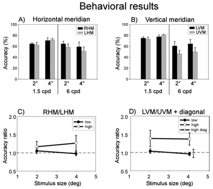
Behavioral performance. A) Accuracy for stimuli on horizontal meridian, averaged across observers. B) Accuracy for stimuli on vertical meridian. C) Horizontal meridian (RHM:LHM) accuracy ratio. The dashed line indicates a ratio of 1, i.e., no difference between the two locations. Open circles, high spatial frequency. Filled circles, low spatial frequency. D) Vertical meridian (LVM:UVM) accuracy ratio and accuracy ratio for diagonal locations. Open circles, high spatial frequency vertical meridian. Filled circles, low spatial frequency vertical meridian. Open triangle, accuracy ratio between the two upper field diagonal locations and the two lower field diagonal locations (horizontal position of the triangle is slightly shifted for better visualization). Error bars, SEM across observers for the main experiment, pooled standard error across observers for the diagonal experiment.
Imaging: activation extent and amplitude
As expected from the known retinotopic organization of early visual areas, vertical meridian stimulation evoked responses in cortical regions on the border of V1 and V2, and horizontal meridian stimulation activated regions in the center of V1 (Figure 3). We focused on these earliest cortical activations in all subsequent analyses.
The extent of activation evoked by the stimuli exhibited a vertical meridian asymmetry, similar to that observed behaviorally (Figure 4). We quantified the activation volumes (number of activated voxels) corresponding to the V1 representations of the right and left horizontal meridian, and corresponding to the upper and lower vertical meridian representations along the V1/V2 borders (Figures 4A, B). There was a larger volume of activity evoked along the lower than the upper vertical meridian, particularly for the high spatial frequency. Then, analogous to the behavioral performance analysis, we computed ratios of the activation volumes for right versus left horizontal meridian, and for upper versus lower vertical meridian (Figures 4C, D). A two-way repeated measures ANOVA with size and spatial frequency as factors was conducted separately for the horizontal and vertical meridian ratios. There was no significant effect for the horizontal meridian (all p > .1). The ANOVA for the vertical meridian ratios revealed a significant main effect of spatial frequency (F(1, 4) = 60.38, p < .01), but no other effects. Furthermore, the extent of activation for the diagonal locations did not exhibit any asymmetry between the upper and lower visual field locations (Figure 4D, open triangle; t(15) = 1.83, p > .05, n = 16 scans across the two observers who participated in the control experiment).
Figure 4.

Extent of cortical activation. A) Activated volume for regions of interest (ROIs) in V1 representing the horizontal meridian, averaged across observers. B) Activated volumes for ROIs representing the vertical meridian. C) Horizontal meridian (RHM:LHM) volume ratio. Open circles, high spatial frequency. Filled circles, low spatial frequency. D) Vertical meridian (LVM:UVM) volume ratio and volume ratio for diagonal locations. Open circles, high spatial frequency vertical meridian. Filled circles, low spatial frequency vertical meridian. Open triangle, volume ratio between the two upper field diagonal locations and the two lower field diagonal locations. Error bars, SEM across observers for the main experiment, pooled standard error across observers for the diagonal experiment.
The fMRI response amplitudes also exhibited a vertical meridian asymmetry (Figure 5). For this analysis, we first defined ROIs from separate (and hence statistically independent) localizer scans for each stimulus location and size. fMRI time series in the main experiment were then extracted from those ROIs and response amplitudes were measured (Figure 5A, B). We computed ratios of the response amplitudes for right versus left horizontal meridian and upper versus lower vertical meridian (Figure 5C, D). Once again, there was no significant effect for the horizontal meridian ratios (all p > .2, two-way repeated measures ANOVA), but a significant effect of spatial frequency for the vertical meridian ratios (F(1, 4) = 28.51, p < .01). Lastly, the fMRI response amplitude did not differ between the upper and lower field locations in the diagonal control experiment (Figure 5D, open triangle; t(15) = 1.45, p > .1, n = 16 scans across the two observers who participated in the control experiment).
Figure 5.

Amplitude of cortical activity (same format as Figure 4). A) Response amplitudes for horizontal meridian. B) Response amplitudes for vertical meridian. C) Horizontal meridian (RHM:LHM) amplitude ratio. D) Vertical meridian (LVM:UVM) amplitude ratio and amplitude ratio for diagonal locations. Error bars, SEM across observers for the main experiment, pooled standard error across observers for the diagonal experiment.
We also conducted the same analyses on the data from individual observers, evaluating statistical significance based on variances calculated from repeated scans of each condition (Figure 6). The same results were obtained for the 4 observers who each completed 2 sessions of data collection. That is, there was no difference between the cortical representations of right and left horizontal meridian, but statistically significant and spatial-frequency dependent differences between both the extent and amplitude of the fMRI measurements in regions corresponding to upper and lower vertical meridian. For the 5th observer who participated in only one scanning session, the results showed the same pattern but did not reach statistical significance, presumably due to a lack of power.
Figure 6.

Example data from an individual observer. Top row, volume ratios. Bottom row, amplitude ratios. Left column, horizontal meridian. Right column, vertical meridian (filled circles, low spatial frequency; open circles, high spatial frequency) and the diagonal locations (triangles). Error bars, SEM across repeated scans. The horizontal position of the triangle is slightly shifted for better visualization.
Discussion
We have found a neural correlate of VMA in the earliest stages of cortical visual processing. Although the behavioral task we adopted in the scanner was different from those typically used in psychophysical studies of VMA, the results are consistent with previous findings: better performance for lower than upper vertical meridian stimuli, but only for high spatial frequency stimuli (Cameron, Tai, & Carrasco, 2002; Carrasco, Talgar, & Cameron, 2001; Carrasco, Williams, & Yeshurun, 2002). Also consistent with these previous studies, we found neither asymmetry along the horizontal meridian nor between upper and lower visual field for diagonal locations. The imaging results in V1/V2 show that both the activation extent and amplitude correlated with the behaviorally-measured VMA. To disambiguate the interpretation of our results, we manipulated the spatial frequency of the stimuli. The importance of this manipulation is discussed below.
A difference between the fMRI response amplitudes at two locations in the brain (e.g., those corresponding to upper versus lower vertical meridian) might reflect differences in the hemodynamics even when the underlying neural responses are the same. Such a difference in hemodynamic gain might, for example, reflect differences in the vasculature (e.g., size or number of veins) between brain regions, a possibility that is likely in our data given the relatively small sizes of our ROIs. Likewise, a difference in the activation extent is confounded by possible differences in the sensitivity (signal-to-noise ratio) of the measurements at two different locations in the brain. Such differences in sensitivity might be caused, for example, by the relative placement of the RF coils and the observer’s head, a possibility that is again likely in our data given that the dorsal V1/V2 border is closer to the surface coil (used to receive the NMR signal) than is the ventral V1/V2 border.
To disambiguate the interpretation of our results, we computed ratios (not differences) of the area and amplitude measures between the two locations on the vertical meridian (lower vs. upper), and we employed three controls. Computing ratios normalized across baseline response levels, and provided relative changes in neural activity across the two locations.
The first control was the spatial frequency manipulation. High spatial frequency stimuli are associated with a larger behavioral asymmetry than are low frequency stimuli (Cameron, Tai, & Carrasco, 2002; Carrasco, Talgar, & Cameron, 2001; Skrandies, 1987). Given that the low and high spatial frequency stimuli occupied the same locations in the visual field and activated the same locations in the brain, any asymmetry in hemodynamic gain would have been the same for the two spatial frequencies. However, consistent with the behavioral asymmetry, our results showed that the neural asymmetry was only present for high spatial frequency stimuli.
The second control was the comparison between horizontal and vertical meridians. Behaviorally, there was no asymmetry for either spatial frequency along the horizontal meridian. This finding is consistent with previous studies (Cameron, Tai, & Carrasco, 2002; Carrasco, Giordano, & McElree, 2004; Carrasco, Talgar, & Cameron, 2001; Carrasco, Williams, & Yeshurun, 2002). The fMRI measurements on the horizontal meridian, for both activation extent and response amplitude, paralleled the behavioral results: there was neither an asymmetry, nor an effect of spatial frequency. These two controls allowed us to rule out potential confounds inherent in the fMRI measurement and reveal the neural asymmetry underling the VMA.
In the third control, we also ruled out an explanation based on a general asymmetry between the upper and lower hemifields (Edgar & Smith, 1990; Previc, 1990). We did not find any behavioral or neural asymmetry between the lower and upper visual field in the control experiment when the stimuli were presented at the diagonal locations. These results demonstrate that the observed neural asymmetry was specific to the vertical meridian.
Given that voluntary attention modulates activity in early visual areas, including V1 (Brefczynski & DeYoe, 1999; Gandhi, Heeger, & Boynton, 1999; Martinez et al., 1999; Somers, Dale, Seiffert, & Tootell, 1999), one should consider whether spatial attention could account for our results. We think it is very unlikely for the following reasons. First, the orientation change targets occurred equally often in all locations, so there was no incentive to preferentially attend to any particular location. Second, a bias to attend preferentially to one of the two stimulus locations would have predicted similar effects for stimuli of both spatial frequencies, whereas our behavioral and neural results depended on stimulus spatial frequency. Third, although covert attention improves overall discriminability, it does not affect the degree of the VMA in a variety of tasks based on contrast sensitivity (Carrasco et al., 2001; Cameron et al., 2002) and spatial resolution (Talgar & Carrasco, 2002) indicating that sensory (not attentional, see (Altpeter, Mackeben, & Trauzettel-Klosinski, 2000; He, Cavanagh, & Intriligator, 1996) factors are responsible for the VMA.
Another possible confound is eye movements. We did not monitor eye movements in the current experiment because our eye tracking system limited the usable field of view for stimulus presentation. However, it is very unlikely that eye movements occurred. First, the observers were trained psychophysical observers and maintained stable fixation in this task when we monitored their eye positions in the psychophysics lab. Second, a bias in eye position (analogous to the bias in attention discussed above) to one of the two stimulus locations would have predicted similar effects for stimuli of both spatial frequencies, whereas our results depended on stimulus spatial frequency. Third, in a pilot experiment using a smaller field of view we recorded eye movements in the scanner with an MRI-compatible eye tracker (ASL Model 504, Applied Science Laboratories, Bedford, MA). We found that observers were able to maintain fixation (see Figure 7) and obtained similar behavioral and imaging results (Liu & Carrasco, Cognitive Neuroscience Society 2005 abstracts). Three of the 5 observers who participated in the current experiment also participated in the pilot experiment.
Figure 7.

Eye position data from a representative observer in a pilot experiment, demonstrating that the observer maintained stable fixation in the scanner. A) and B) horizontal eye position. C) and D) vertical eye position. Color shaded regions in all panels indicate ±1 standard deviation across 6 scans. The two horizontal dashed lines indicate ±1° around the fixation. Eye position was recorded at 60 Hz with an infrared video camera (Model 504LRO; Applied Sciences Laboratories, http://www.a-s-l.com), and plotted after removing blinks and artifacts. During the first 9 s (indicated by the gray rectangle in panels B and C and magnified in panels A and D), observers were instructed to follow a dot target that alternated its location between fixation and one of the four diagonal locations (5° eccentricity). After the instructed saccades, the scan commenced for 200 sec while stimuli were presented on the vertical meridian at 5° of eccentricity in a block alternation protocol. The observer performed the same detection/discrimination task as in the main experiment while maintaining central fixation. Accuracy was comparable to that of the present experiment.
Our fMRI results could be due to either a larger number of cortical neurons responding to stimuli in the lower than the upper portion of the vertical meridian – the “area hypothesis”, or larger response amplitudes for the lower than the upper vertical meridian stimuli – “amplitude hypothesis”. Both accounts – pooling across a larger number of neurons and relying on a larger neuronal response – can give rise to an enhanced behavioral sensitivity for lower than upper vertical meridian representation. We present some preliminary modeling work in the Appendix aimed at distinguishing between these two possibilities.
Conclusions
In summary, we found that neural asymmetries correlated with the VMA arise at the earliest stage of cortical visual processing. Both the extent and amplitude of activation in V1/V2 showed a dorsal vs. ventral asymmetry corresponding to the behavioral asymmetry. These results further demonstrate that visual performance could be limited by the pooled sensory responses of large populations of neurons in visual cortex.
Acknowledgments
We thank Cheryl Olman and Souheil Inati for help with MR protocol optimization, and Stuart Fuller, Shani Offen and Denis Schluppeck for comments on this manuscript. This research was supported by the National Eye Institute Grant R01-EY11794, and a grant from the Seaver Foundation to NYU.
Commercial relationships: none.
Appendix
We found that both the extent and amplitude of fMRI activation correlated with VMA. These results suggest, but do not necessarily imply, that the underlying neural activity exhibit both larger extent (“area hypothesis”) and higher response amplitudes (“amplitude hypothesis”). Empirically, it is difficult to distinguish these alternatives with any non-invasive techniques (fMRI, ERP, and MEG) that measure the aggregate neural activity over many neurons. The spatial dispersion (blurring) of the hemodynamic response presents a challenge for unambiguously distinguishing between these two hypotheses. Here we illustrate our attempt to distinguishing the area and the amplitude hypotheses by using two stimulus sizes and fitting the data with a simple model. For simplicity/parsimony, our model assumes that the neuronal density is constant, although it is possible that the neuronal density is higher for the lower than the upper vertical meridian stimuli, with equal extent of neural tissue and response amplitude.
General framework of the model
The spatial blurring of the fMRI measurements was modeled as a shift-invariant linear system, i.e., as a convolution of the neural activity with a point-spread function (Engel, Glover, & Wandell, 1997). Specifically, the hypothetical neural activity (Figure A1, left column) was convolved with a Gaussian filter (middle column) to yield the fMRI response (right column). The shape of the hemodynamic spread was assumed to be constant, independent of the magnitude of the neural response. Furthermore, we assumed that the hemodynamic responses increased monotonically with the underlying neural activity but the model did not depend on a strictly linear relationship between neural activity and hemodynamic response (e.g., the hemodynamics could exhibit an initial expansive nonlinearity at low levels of neural activity followed by a compressive nonlinearity as the neural activity increased). We selected a threshold level of the simulated fMRI response, which was equivalent to adopting a particular statistical threshold (p value) in analyzing the fMRI data. Finally, the extent of activation was defined as the square of the region covered by the suprathreshold activity (because the simulation was conducted in 1-dimension whereas actual hemodynamic spread occur on 2-dimensional cortical surfaces), and the response amplitude was defined as the average response magnitude for all suprathreshold points.
Figure A1.

Schematic of the model. Left column, hypothesized spatial distribution of the underlying neural activity as a function of cortical position. The middle column represents the blurring effect of the hemodynamics. Right column, simulated fMRI responses computed by convolution of the first two columns. All panels within a column are in the same scale. The three rows represent different scenarios of cortical activity. First row, reference condition. Second row, wider extent of cortical activity but with the same amplitude as the reference condition. Third row, higher amplitude but with the same extent of cortical activity as the reference condition.
As an illustration of the potential confound between the area and amplitude hypotheses, consider the three scenarios depicted in the three rows in Figure A1. The first row shows a reference condition, the second row corresponds to the same amplitude of neural activity as the first row but with a larger extent, and the third row corresponds to the same extent of neural activity but with a higher amplitude. As can be seen in the figure, the extent of the simulated fMRI activation in both the second and third rows is larger than that in the first row. Likewise, the peaks of the simulated fMRI response amplitudes in the two bottom rows are higher than that in the first row. Thus a change in the extent or the amplitude of underlying neural activity might produce similar effects in the fMRI measurements.
We manipulated stimulus size in the experiment in an attempt to disambiguate amplitude and extent. Changing the stimulus size (in a retinotopically-organized visual area) changes the extent of neural activity, but does not affect the hemodynamic filter, thereby offering the opportunity to dissociate the two effects. In the extreme case where the neural activity has a much larger size than the hemodynamic filter, the effect of hemodynamic blurring would be negligible. Hence, the neural asymmetry should exhibit different signatures as a function of stimulus size depending on whether the area hypothesis or amplitude hypothesis is correct.
Modeling procedures
We simulated the extent and amplitude of activation for the low and high spatial frequency stimuli at the upper and lower vertical meridian. Volume and amplitude ratios were then calculated and compared to measured data. We could not directly estimate model parameters via iterative fitting methods because the model contains highly non-linear operations (e.g., thresholds, ratios). Instead, an exhaustive search procedure was used to match the data as closely as possible, separately for the area and amplitude models, by systematically exploring 4 parameters: amount of asymmetry for the low spatial frequency stimuli, amount of asymmetry for the high spatial frequency stimuli, spread of the hemodynamic filter, and threshold. In addition, we evaluated a hybrid model, in which there were both area and amplitude asymmetries in neural activity. The hybrid model contained one more parameter: the proportion of asymmetry contributed by area asymmetry vs. amplitude asymmetry.
These parameters were varied in a range at 20–40 discreet values, while cortical magnification at our stimulus eccentricity (6°) was fixed at 2.2 mm/deg, using the formula from a previous fMRI study (Duncan & Boynton, 2003). Given a particular combination of the parameters, the volume and amplitude ratios were calculated and compared to the measured data – 4 ratio values (2 sizes × 2 spatial frequency). To evaluate the goodness of the fit, we calculated the sum of the squared errors weighted by the inverse of the variance of the measured data point. We started with a large parameter range and a coarse sampling of each parameter value. After obtaining the goodness of fit, we narrowed the parameter space based on the 500 best fitting parameter combinations and re-ran the simulation with finer sampling over a more limited range of parameter values. We repeated this step twice, evaluating a total of more than 1 million model parameter combinations in each simulation.
Modeling results
In Figure A2, we show examples of three different models and their fit to the data. We were not able to fit the data well with either a pure area model or an amplitude model. The area model tended to fit the area ratio data better than the amplitude ratio and the amplitude model tended to fit the amplitude ratio better than the area ratio. We achieved a better fit with a hybrid model, which fit both set of ratios reasonable well (see the R2 values in the figure). The superior fit of the hybrid model is not surprising given that it has one more free parameter. Furthermore, the proportion of area vs. amplitude asymmetry for the best fitting models varied greatly (50%–75%, the model depicted in panel E, F had equal contribution from both asymmetries). Due to these considerations, we cannot draw firm conclusions regarding the neural asymmetry underlying the asymmetry in fMRI measurements.
Figure A2.

Model simulation results. A) and B) Simulated volume and amplitude ratios as a function of stimulus size for the area model; C) and D) same data for the amplitude model, E) and F) same data for the hybrid model. Actual data (triangles with error bars) were superimposed on the simulation results. Inset in each panel indicates the percent of variance in the data accounted for by the model.
Modeling Conclusion
Although varying the stimulus size in theory allows one to distinguish the area vs. amplitude hypothesis, our data do not readily conform to either model prediction. We offer a hybrid model that fits the data reasonably well but we do not claim that neural asymmetries in both area and amplitude underlie the VMA.
Our experimental and modeling work indicate that it is non-trivial to disentangle the area and amplitude hypotheses. Such a distinction is important in certain domains of research, e.g., perceptual learning (Furmanski et al., 2004) and sensory deprivation (Fine et al., 2005). Although our results did not yield an unambiguous interpretation, further experimentation and modeling using similar approaches will shed more light on this issue.
Contributor Information
Taosheng Liu, Department of Psychology and Center for Neural Science, New York University, New York, NY, USA.
David J. Heeger, Department of Psychology and Center for Neural Science, New York University, New York, NY, USA
Marisa Carrasco, Department of Psychology and Center for Neural Science, New York University, New York, NY, USA.
References
- Altpeter E, Mackeben M, Trauzettel-Klosinski S. The importance of sustained attention for patients with maculopathies. Vision Research. 2000;40(10–12):1539–1547. doi: 10.1016/s0042-6989(00)00059-6. [DOI] [PubMed] [Google Scholar]
- Brainard DH. The Psychophysics Toolbox. Spat Vis. 1997;10(4):433–436. [PubMed] [Google Scholar]
- Brefczynski JA, DeYoe EA. A physiological correlate of the ‘spotlight’ of visual attention. Nat Neurosci. 1999;2(4):370–374. doi: 10.1038/7280. [DOI] [PubMed] [Google Scholar]
- Cameron EL, Tai JC, Carrasco M. Covert attention affects the psychometric function of contrast sensitivity. Vision Res. 2002;42(8):949–967. doi: 10.1016/s0042-6989(02)00039-1. [DOI] [PubMed] [Google Scholar]
- Carrasco M, Giordano AM, McElree B. Temporal performance fields: visual and attentional factors. Vision Res. 2004;44(12):1351–1365. doi: 10.1016/j.visres.2003.11.026. [DOI] [PubMed] [Google Scholar]
- Carrasco M, Talgar CP, Cameron EL. Characterizing visual performance fields: effects of transient covert attention, spatial frequency, eccentricity, task and set size. Spat Vis. 2001;15(1):61–75. doi: 10.1163/15685680152692015. [DOI] [PMC free article] [PubMed] [Google Scholar]
- Carrasco M, Williams PE, Yeshurun Y. Covert attention increases spatial resolution with or without masks: support for signal enhancement. J Vis. 2002;2(6):467–479. doi: 10.1167/2.6.4. [DOI] [PubMed] [Google Scholar]
- Connolly M, Van Essen D. The representation of the visual field in parvicellular and magnocellular layers of the lateral geniculate nucleus in the macaque monkey. J Comp Neurol. 1984;226(4):544–564. doi: 10.1002/cne.902260408. [DOI] [PubMed] [Google Scholar]
- DeValois RL, DeValois KK. Spatial vision. New York: Oxford University Press; 1988. [Google Scholar]
- DeYoe EA, Carman GJ, Bandettini P, Glickman S, Wieser J, Cox R, et al. Mapping striate and extrastriate visual areas in human cerebral cortex. Proc Natl Acad Sci U S A. 1996;93(6):2382–2386. doi: 10.1073/pnas.93.6.2382. [DOI] [PMC free article] [PubMed] [Google Scholar]
- Duncan RO, Boynton GM. Cortical magnification within human primary visual cortex correlates with acuity thresholds. Neuron. 2003;38(4):659–671. doi: 10.1016/s0896-6273(03)00265-4. [DOI] [PubMed] [Google Scholar]
- Edgar GK, Smith AT. Hemifield differences in perceived spatial frequency. Perception. 1990;19(6):759–766. doi: 10.1068/p190759. [DOI] [PubMed] [Google Scholar]
- Engel SA, Glover GH, Wandell BA. Retinotopic organization in human visual cortex and the spatial precision of functional MRI. Cereb Cortex. 1997;7(2):181–192. doi: 10.1093/cercor/7.2.181. [DOI] [PubMed] [Google Scholar]
- Engel SA, Rumelhart DE, Wandell BA, Lee AT, Glover GH, Chichilnisky EJ, et al. fMRI of human visual cortex. Nature. 1994;369(6481):525. doi: 10.1038/369525a0. [DOI] [PubMed] [Google Scholar]
- Fine I, Finney EM, Boynton GM, Dobkins KR. Comparing the Effects of Auditory Deprivation and Sign Language within the Auditory and Visual Cortex. J Cogn Neurosci. 2005;17(10):1621–1637. doi: 10.1162/089892905774597173. [DOI] [PubMed] [Google Scholar]
- Furmanski CS, Schluppeck D, Engel SA. Learning strengthens the response of primary visual cortex to simple patterns. Curr Biol. 2004;14(7):573–578. doi: 10.1016/j.cub.2004.03.032. [DOI] [PubMed] [Google Scholar]
- Fleysher L, Fleysher R, Heeger DJ, Inati S. High resolution fMRI using a 3D multi-shot EPI sequence. Proc Intl Soc Magn Reson Med. 2005;13:2685. [Google Scholar]
- Gandhi SP, Heeger DJ, Boynton GM. Spatial attention affects brain activity in human primary visual cortex. Proc Natl Acad Sci U S A. 1999;96(6):3314–3319. doi: 10.1073/pnas.96.6.3314. [DOI] [PMC free article] [PubMed] [Google Scholar]
- He S, Cavanagh P, Intriligator J. Attentional resolution and the locus of visual awareness. Nature. 1996;383(6598):334–337. doi: 10.1038/383334a0. [DOI] [PubMed] [Google Scholar]
- Heeger DJ, Boynton GM, Demb JB, Seidemann E, Newsome WT. Motion opponency in visual cortex. J Neurosci. 1999;19(16):7162–7174. doi: 10.1523/JNEUROSCI.19-16-07162.1999. [DOI] [PMC free article] [PubMed] [Google Scholar]
- Levine MW, McAnany JJ. The relative capabilities of the upper and lower visual hemifields. Vision Res. 2005;45(21):2820–2830. doi: 10.1016/j.visres.2005.04.001. [DOI] [PubMed] [Google Scholar]
- Martinez A, Anllo-Vento L, Sereno MI, Frank LR, Buxton RB, Dubowitz DJ, et al. Involvement of striate and extrastriate visual cortical areas in spatial attention. Nat Neurosci. 1999;2(4):364–369. doi: 10.1038/7274. [DOI] [PubMed] [Google Scholar]
- Maunsell JHR, Van Essen DC. Topographic organization of the middle temporal visual area in the macaque monkey: representational biases and the relationship to callosal connections and myeloarchitectonic boundaries. J Comp Neurol. 1987;266(4):535–555. doi: 10.1002/cne.902660407. [DOI] [PubMed] [Google Scholar]
- Pelli DG. The VideoToolbox software for visual psychophysics: transforming numbers into movies. Spat Vis. 1997;10(4):437–442. [PubMed] [Google Scholar]
- Perry VH, Cowey A. The ganglion cell and cone distributions in the monkey’s retina: implications for central magnification factors. Vision Research. 1985;25(12):1795–1810. doi: 10.1016/0042-6989(85)90004-5. [DOI] [PubMed] [Google Scholar]
- Portin K, Vanni S, Virsu V, Hari R. Stronger occipital cortical activation to lower than upper visual field stimuli. Neuro-magnetic recordings. Exp Brain Res. 1999;124(3):287–294. doi: 10.1007/s002210050625. [DOI] [PubMed] [Google Scholar]
- Previc FH. Functional specialisation in the lower and upper visual fields in humans: its ecological origins and neurophysiological implications. Behav Brain Sci. 1990;13:519–575. [Google Scholar]
- Rubin N, Nakayama K, Shapley R. Enhanced perception of illusory contours in the lower versus upper visual hemifields. Science. 1996;271(5249):651–653. doi: 10.1126/science.271.5249.651. [DOI] [PubMed] [Google Scholar]
- Sereno MI, Dale AM, Reppas JB, Kwong KK, Belliveau JW, Brady TJ, et al. Borders of multiple visual areas in humans revealed by functional magnetic resonance imaging. Science. 1995;268(5212):889–893. doi: 10.1126/science.7754376. [DOI] [PubMed] [Google Scholar]
- Skrandies W. The upper and lower visual field of man: electro-physiological and functional differences. In: Ottoson D, editor. Progress in sensory physiology. Berlin: Springer; 1987. pp. 1–93. [Google Scholar]
- Slotnick SD, Yantis S. Efficient acquisition of human retinotopic maps. Hum Brain Mapp. 2003;18(1):22–29. doi: 10.1002/hbm.10077. [DOI] [PMC free article] [PubMed] [Google Scholar]
- Somers DC, Dale AM, Seiffert AE, Tootell RB. Functional MRI reveals spatially specific attentional modulation in human primary visual cortex. Proc Natl Acad Sci U S A. 1999;96(4):1663–1668. doi: 10.1073/pnas.96.4.1663. [DOI] [PMC free article] [PubMed] [Google Scholar]
- Talairach J, Tournoux P. Co-planar Sterotaxic Atlas of the Human Brain. New York: Thieme; 1988. [Google Scholar]
- Talgar CP, Carrasco M. Vertical meridian asymmetry in spatial resolution: visual and attentional factors. Psychon Bull Rev. 2002;9(4):714–722. doi: 10.3758/bf03196326. [DOI] [PubMed] [Google Scholar]
- Tootell RB, Switkes E, Silverman MS, Hamilton SL. Functional anatomy of macaque striate cortex. II. Retinotopic organization. J Neurosci. 1988;8(5):1531–1568. doi: 10.1523/JNEUROSCI.08-05-01531.1988. [DOI] [PMC free article] [PubMed] [Google Scholar]
- Van Essen DC, Newsome WT, Maunsell JHR. The visual field representation in striate cortex of the macaque monkey: asymmetries, anisotropies, and individual variability. Vision Res. 1984;24(5):429–448. doi: 10.1016/0042-6989(84)90041-5. [DOI] [PubMed] [Google Scholar]