Functional Connectivity in fMRI: A Modeling Approach for Estimation and for Relating to Local Circuits

Abstract

Although progress has been made in relating neuronal events to changes in brain metabolism and blood flow, the interpretation of functional neuroimaging data in terms of the underlying brain circuits is still poorly understood. Computational modeling of connection patterns both among and within regions can be helpful in this interpretation. We present a neural network model of the ventral visual pathway and its relevant functional connections. This includes a new learning method that adjusts the magnitude of interregional connections in order to match experimental results of an arbitrary functional magnetic resonance imaging (fMRI) data set. We demonstrate that this method finds the appropriate connection strengths when trained on a model system with known, randomly chosen connection weights. We then use the method for examining fMRI results from a one-back matching task in human subjects, both healthy and those with schizophrenia. The results discovered by the learning method support previous findings of a disconnection between left temporal and frontal cortices in the group with schizophrenia, and a concomitant increase of right-sided temporo-frontal connection strengths. We then demonstrate that the disconnection may be explained by reduced local recurrent circuitry in frontal cortex. This method extends currently available methods for estimating functional connectivity from human imaging data by including both local circuits and features of inter-regional connections, such as topography and sparseness, in addition to total connection strengths. Furthermore, our results suggest how fronto-temporal functional disconnection in schizophrenia can result from reduced local synaptic connections within frontal cortex rather than compromised inter-regional connections.

INTRODUCTION

One of the more difficult aspects of making effective use of functional neuroimaging methods is in the interpretation of results in terms of the underlying brain functions. There are multiple reasons for this, including the disparities of scale in both temporal and spatial resolution, and differences between what is being measured in imaging and in non-human studies such as electrophysiology. Imaging methods such as positron emission tomography (PET) and functional magnetic resonance imaging (fMRI) originally focused on identifying brain locations that are more active in one condition than in another. More recently, fMRI has increased both the spatial and temporal resolution at which imaging data is acquired, and more interest has been directed toward examining interactions among brain regions. Currently, the prevailing view is that brain function is best characterized as a balance between local specialization and interactions among widespread regions. However, the factors that influence the functional connectivity as measured by PET and fMRI, and its relationship to regional circuitry are poorly understood.

Computational modeling is one method that has recently been applied toward examining relationships between underlying brain mechanisms and the observed brain imaging data (Arbib et al., 1995; Tagamets & Horwitz, 1998; Corchs & Deco, 2002; Corchs & Deco, 2004). We have previously developed a large-scale neuronal network model that attempts to bridge the gap between events at the neuronal level and human imaging methods, such as PET and fMRI, by representing regions as groups of neural populations at the column level (Tagamets & Horwitz, 1998; Tagamets & Horwitz, 2000; Tagamets & Horwitz, 2001). To date this and other models of fMRI have been used for modeling regional brain activations in terms of underlying neuronal dynamics, but in those models that include multiple brain regions, including ours, the connectivity among regions was estimated from data in the non-human primate literature and refined by adjusting these weights by hand to match human empirical data. However, in order to investigate mechanisms for differences between tasks or groups, it can be useful to quantitatively match a specific fMRI data set, e.g. healthy control subjects, then examine other parameters in the model that best explain a comparison data set, such as that from a patient population. Here we present such an approach to examining differences between healthy controls and persons with schizophrenia during fMRI tasks of single word processing.

We describe a neuronal network model of two hemispheres and a new learning method that finds a set of inter-regional connection weights that allows the model to reproduce activation values in a specific imaging data set. Using simulated data sets with known connectivity, we demonstrate convergence and uniqueness of the learned weights. We then demonstrate the use of this method on a set of fMRI data, comparing connectivity in healthy control and schizophrenic volunteers as they perform a simple word-matching task. Finally, we examine the interactions of local (within-region) circuits with brain activations and interregional functional connectivity in fMRI data. We show that functional connectivity between brain regions can be disproportionately affected, as compared to activation, by properties of local circuits. We conclude that this combined theory-driven and data-driven methodology extends current imaging analysis methods and allows examination of properties other than total activations and functional interregional connection strengths.

BACKGROUND

To date, methods for estimating functional and effective connectivity from brain imaging data can generally be classified into two types: Those that look for groupings of regions that work together without regard to how they are connected (Cordes et al., 2000; Arfanakis et al., 2000; Calhoun et al., 2001; Calhoun et al., 2005), and those that rely on an underlying model of connection patterns among a specific set of regions and connections that are hypothesized to mediate the task of interest (McIntosh & Gonzalez-Lima, 1994; Friston et al., 2003). While the former are purely data-driven, the latter methods are based on hypotheses about specific networks that are important in mediating the task under consideration, and the goal is to find connection strengths that satisfy the constraints of the imaging data. To date these network-based methods have been built of modules that represent whole regions of the brain as simple components with no internal structure. Although some recent methods have taken account of the indirect relationship between neuronal activity and hemodynamic response (Friston et al., 2003), brain regions in these models are still represented by a single variable, the cumulative activity of a large set of neural populations in a region. Furthermore, methods such as structural equation modeling (SEM(McIntosh & Gonzalez-Lima, 1992; McIntosh & Gonzalez-Lima, 1994) and dynamic causal modeling (DCM; (Friston et al., 2003) do not take synaptic inhibition and energetic consequences of modulatory neurotransmitter effects into account. For example, how synaptic inhibition affects local blood flow (fMRI signal) is not well understood (Jueptner & Weiller, 1995; Magistretti & Pellerin, 1999; Logothetis et al., 2001; Caesar et al., 2003). Because of this, a positive connection weight can not necessarily be interpreted as an excitatory underlying connection. Finally, these methods do not take other effects such as the geometry and local properties of inter-regional connections or local circuitry into account. An important and often neglected aspect of neuroimaging data is that the measured regional blood flow (rCBF) seen in PET and the blood oxygen dependent (BOLD) effect seen in fMRI reflect a large local response to a possibly weak long-range input to a region, since most cortico-cortical connections are local (Douglas et al., 1995; Tagamets & Horwitz, 1998). Consequently, the interpretation of imaging connectivity data can be enhanced by the ability to examine the relationships between local and inter-regional circuit effects.

In a variety of clinical populations with brain disorders, differences in local circuits are likely to explain at least part if not all of the difference in activations and inter-regional connection values. For example, reduction in functional connectivity between frontal and posterior has been found in a number of imaging studies of schizophrenia (Dolan et al., 1995; Fletcher et al., 1996; Lawrie et al., 2002; Ragland et al., 2004). While evidence for deficits in white matter tracts between these regions is inconsistent (McGuire & Frith, 1996), there is evidence of local circuit disturbances in frontal cortex (Lewis & Gonzalez-Burgos, 2000; Glantz & Lewis, 2000; Kolluri et al., 2005). We will examine the hypothesis that reduced local connections in frontal cortex can reduce functional connectivity as measured by fMRI.

Our previous modeling results suggest that the interaction of local circuitry and the context of converging excitatory and inhibitory neuronal activity is likely to influence imaging data (Tagamets & Horwitz, 2001). The effect of afferent neuronal context has recently been supported by electrophysiological experiments in the rat cerebellum (Caesar et al., 2003), where it was shown that simultaneously converging excitatory and inhibitory inputs to a region result in a smaller change in local blood flow than would be expected if they were purely additive. Our own modeling results also suggest that how such simultaneous inputs are reflected in regional metabolsim depends on the amount of local excitatory recurrence in the region (Tagamets & Horwitz, 2001). Because most synapses are local, it is likely that both regional activations and inter-regional correlations in brain imaging data are strongly dependent on the nature of these local circuits. Modeling these explicitly will allow us to account for these effects and examine the role they play in the observed imaging data.

To date, there have been only a few attempts at modeling imaging data. The earliest modeling study of human functional imaging data, referred to as synthetic pet, computed PET data during a simulated saccade task by summing the absolute values of afferent synaptic activities within the areas of the model (Arbib et al., 1995). Part of the purpose of their study was to test the hypothesis that inhibitory afferent synaptic activities can produce an increase in PET activity, an effect that has been suggested by both experimental and theoretical studies (Ackermann et al., 1984; Horwitz & Sporns, 1994; Jueptner & Weiller, 1995). That this turned out to be the case in their model emphasizes the potentially counterintuitive nature of interpreting imaging data.

Our own previous work with modeling functional imaging data has been directed at gaining a better understanding of both the quantitative and qualitative properties of this data. The original goal was to have a model based on underlying neural circuitry be able to perform the task, for neuronal elements in the model to behave similarly to electrophysiological recordings in non-human primates, and to yield quantitative data similar to imaging activations at the regional level. The initial model included regions in the ventral visual pathway and performed a delayed match-to-sample task. We have studied inter-regional connectivity in the model by examining how it is affected by two parameters: familiarity of the stimulus and the attentional modulation of prefrontal cortex during the delayed match-to-sample task (Horwitz et al., 1999; Horwitz et al., 2005). The results suggested that connectivity is strongest in the presence of high attention and familiar stimuli. The relevance of familiarity was modeled by first training the model on specific input items by a competitive Hebbian learning rule (Tagamets & Horwitz, 1998), while attention was modeled by changing the response dynamics of local neuronal populations (Tagamets & Horwitz, 2000). The Hebbian learning redistributes the inter-regional connection weights to sharpen the encoding of learned items, without changing the total connection weights between regions. This model demonstrated that measured connectivity in imaging data can be affected by the topography of the connections even when total physical connectivity strength remains the same.

To date, we have not addressed the issue of data-driven estimation of inter-regional connectivity strengths for the model. Rather, our estimates were based on experimental data from the anatomical animal literature, with manual adjustments made to account for a specific experimental imaging study (Tagamets et al., 1998). In this paper, we present a new method that we have developed for automated estimation of connection strengths for the model from an arbitrary fMRI data set. This problem differs from the usual supervised learning methods in neural networks in that there are target values for all regions in the network, not just for an output “layer.” This method allows estimation of functional connectivity while allowing for effects of the interaction of interregional and local circuits. It differs from other measures of functional connectivity currently in use in two major ways. First, the model itself is a generative one that attempts to explain how imaging data such as rCBF and BOLD signal can be related to underlying neural mechanisms. Second, the connection training method is based on matching average activations in the regions of interest (ROIs), as opposed to other methods such as structural equation modeling (McIntosh & Gonzalez-Lima, 1992; McIntosh & Gonzalez-Lima, 1994), partial least squares (McIntosh, 1998; McIntosh et al., 2004; McIntosh & Lobaugh, 2004), and DCM (Friston et al., 2003; Mechelli et al., 2003; Penny et al., 2004), which derive effective connection strengths from covariances or correlations that are computed from the data. We posit that average within-task activations are computed more reliably than within-task covariances in event-related fMRI data. In the latter, in order to remain with-task, the covariances have to be computed over the maxima of widely spaced response peaks. Given the uncertainty about causes of variability of the hemodynamic delay, magnetic drift, and other factors in fMRI data, it is unclear how best to capture exactly where and when these maxima occur.

METHODS

Description of the model

The original model (Tagamets & Horwitz, 1998) employed a visual delayed match-to-sample circuit that detected repeated stimuli that were encoded along a path of several regions modeling the functions of their counterparts in the human brain. This model included only a single hemisphere. Stimuli are passed from an input region (lateral geniculate nucleus, LGN, not explicitly modeled) to the prefrontal cortex via modeled regions corresponding to V1/V2, V4, and inferior temporal cortex (TEO/IT), in that order, the progression breaking stimuli into pieces, distributing feature information throughout the areas, and encoding stimuli. A prefrontal (PFC) region implements a form of working memory, which maintains stimuli online and makes decisions about matches.

We now extend the model to include additional regions and other additions. There are now left and a right hemispheres with symmetric regions. Because the task that we are modeling is lateralized to the left, and because the functional disconnectivity seen in schizophrenia is mostly confined to the left hemisphere, V2 was separated from V1 in the model. This is because V1 has no callosal connections, while V2 is known to have callosal connections, and these factors are likely to affect lateralization. Dividing the V1/V2 area of the model into distinct populations of V1 and V2 hypercolumns also adds a further encoding and distribution of feature information to the model. A hippocampal region (HC), which has been demonstrated to become more active during the fMRI task we are modeling, and which is thought to be implicated in schizophrenia, has also been added to the model (see Figure 1). It has bi-directional connections with both areas TEO/IT and the prefrontal cortex. In the original model, stimuli were simple shapes. Because we now want to model strings of letters that simulate the experimental conditions of our study, the regions are larger than in the original model, with more basic units in each region. Stimuli are four-letter words, and are made up from symbols that resemble real alphabetic letters (see the LGN input areas in Figure 3 for an example of a single 4-letter stimulus). Real words and non-words are represented by strings that have and have not been trained, respectively, with a competitive Hebbian learning method. In a manner that is analogous to the human visual system, the right half of the stimulus goes to the model's left hemisphere and the left half of the stimulus goes to the right. Finally, a decision circuit that detects both matches and non-matches has been added.

Figure 1.

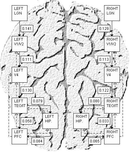
The model at the resolution of the included regions, and the feed-forward and feedback pathways between them. Feed-forward pathways are indicated by solid arrows, while feedback pathways are indicated by dashed arrows. The connection weights pictured are the average incoming weights to a unit in the destination region from all units in the source region after training with the gains learning algorithm (see the Methods and Results sections). These weights represent the estimated interregional connection weights of the healthy volunteer group in a delayed match-to-sample task with real words.

Figure 3.

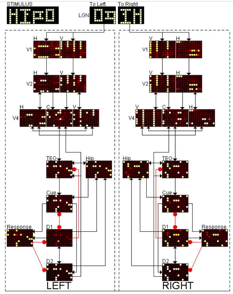
Snapshot of the running model at the resolution of the hypercolumns, and separated into distinct regions and subpopulations. This picture was taken at the end of the response period where the second stimulus, HIPO, matched the first stimulus. On both the left and right, the response units are activated sufficiently to indicate the model recognizes a match. Excitatory connections end in arrows, while the inhibitory connections end in a circle. Not depicted are self excitatory and inhibitory connections or callosal connections.

As in the original model, each region consists of units (see Figure 2A) that are examples of the Wilson-Cowan unit (Wilson & Cowan, 1972), with local circuit connection strengths derived from the animal literature (Douglas et al., 1995). A unit's neuronal activation at any time is computed as a sigmoid function of the sum of the weighted incoming activity, including self connections. In addition, absolute values of all synaptic inputs to a unit are summed over the entire task period, over all units in a region, to yield a measure that corresponds to the modeled rCBF or BOLD response for that region.

Figure 2.

Local circuit level components of the model.

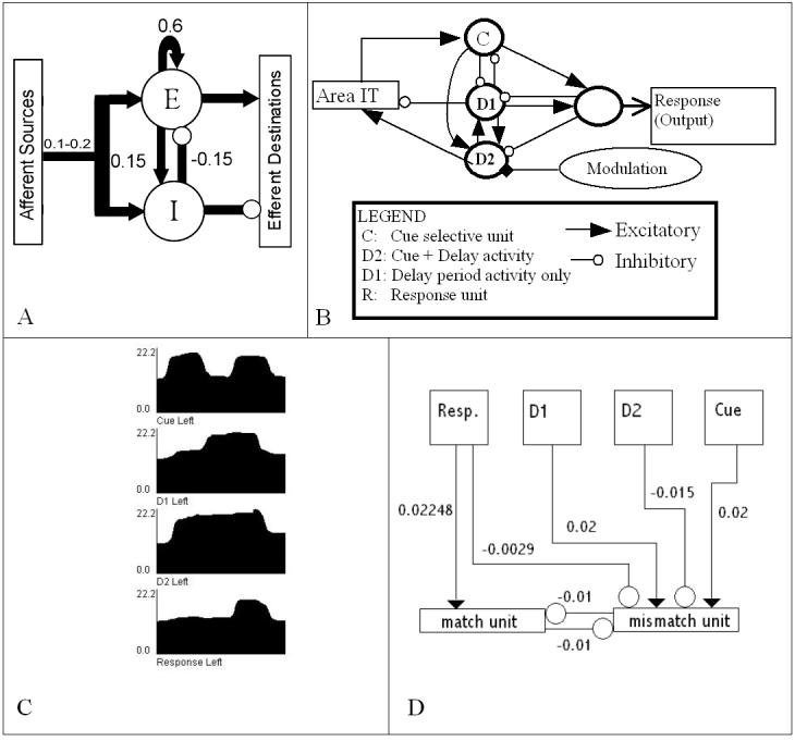
1. Representation of a single unit in the model. Total synaptic activity adds up to about 1.0, and each connection strength represents an approximate percentage of the total synaptic activity of the unit. Incoming connections from other regions typically account for anywhere from 10 to 20% of a unit's total activity.
2. The working memory circuit in the PFC region of the model. Stimuli enter the circuit via the Cue units (C). D1 and D2 units maintain delay period activity, and the response unit activates only when the current stimulus matches the one held in memory.
3. Dynamics of the four types of units in the WM circuit. x-axis: Time. y-axis: Summed neural activity of all units. The Cue units are activy only when a stimulus is present. D1 and D2 units maintain delay period activity (see text). Response units activate only if the current stimulus matches the one held in working memory.
4. Diagram of the connection strengths from each unit of the prefrontal cortex into the two decision units, match and mismatch. Match and mismatch units are tracked during the response period and whichever one is higher for the sum over both hemispheres is the decision the model makes about the task performed during that trial. The match and mismatch units inhibit one another. The response units are the sole source of excitation of the match unit, and they inhibit the mismatch units. The mismatch unit is excited by Cue and D1 units. The activity of the mismatch unit will be larger for words that have a stronger neural representation and aids in preventing false positives for matches based only on the number of units excited rather than the response to matching patterns. D2 inhibits the mismatch unit so there is not too much excitation in the mismatch in the first two stages of the task.

The prefrontal cortex circuit (Figure 2B), which performs the delayed match-to-sample task in the model, was intended to capture the function of working memory, with neural responses (Figure 2C) that mimic the dynamics of single cells found in monkey prefrontal cortex during different phases of a delayed match-sample task (Funahashi et al., 1990; Goldman-Rakic, 1995). In addition to the maintenance part of working memory, it includes a population of neurons that implements decision-making in the delayed match-to-sample task, and these populations further interact with the maintenance circuit to facilitate working memory updating. The response units have inhibitory connections into the delay units, so that a matching stimulus tends to erase maintenance of the stimulus in working memory unless counteracted by other factors, such as a higher attention level to that stimulus. Thus, the circuit implements not only maintenance, but also decision-making and updating encodings in working memory.

The model's task is detecting a match between a first stimulus held in working memory in the prefrontal cortex and a later stimulus presented after a delay, with possible intervening non-matching stimuli. A new feature of the model is the addition of a non-match decision unit for each hemisphere, in addition to the match decision units that were in the original version (see Figure 2D). If the total values of both match units exceed that of the mismatch units for a given trial, the model indicates a match has been presented. Otherwise, the mismatch units fire, indicating a mismatch between the first and second stimuli.

The model undertakes the task in four stages, each one lasting 200 iterations, which is taken to be the equivalent of one second of real time. These phases are: a first stimulus or cue period, a delay period, a second stimulus or response period, and an intertrial period before the next task. The summed neuronal activities for the subpopulations in the WM circuit during these phases are shown in Figure 2C, and their dynamics are described below.

The cue period is first, during which the LGN contains the first stimulus. Activity is propagated through the V1, V2 and then V4 regions, which break down the stimulus into vertical lines, horizontal lines, and in the case of V4, corners as well. This is passed on to the TEO/IT region, which stores an encoded representation of the entire object. Activity then moves to the prefrontal cortex, both directly and via the hippocampus. During the second stage, the delay period, the stimulus is no longer present in the LGN. Activity in the V1/V2, V4, TEO/IT, and hippocampus diminishes, while the cue units in the prefrontal cortex also lose their activity. At this point the D2 units remain active, and they trigger the D1 units to become active during the delay period after the inhibitory effect from the cue units onto D1 is reduced. Modulation by an “attentional” mechanism, which is likely to be mediated by dopamine, is to the D2 units only (see Figure 2B). Together the D1 and D2 units sustain the memory of the stimulus during the delay period. During this period, feedback from the D2 units into area TEO/IT sustains sub-threshold activity in the pathway, and feedback from TEO/IT into more posterior regions propagates this effect. We hypothesize that this mechanism enables units along the whole pathway to respond more quickly to the next matching stimulus, and is the mechanism responsible for the frequently observed increases in activity in sensory association areas during tasks that require attention to specific features.

When the response period follows, a second stimulus is presented to the model in the LGN, and as in the cue period, activity propagates forward through the V1, V2, V4, TEO/IT, and hippocampal regions. The cue units in the prefrontal cortex are activated. Corresponding units that match in the cue and D1 units trigger activity in the response units. The closer the cue and D1 match, the greater the response. Activity in response units is thus higher when the first and second patterns are identical or similar, and lower when the two patterns do not match. These response units, in turn, inhibit the D1 and D2 units, and erase the memory once a decision has been made. Figure 3 shows a snapshot of the response period in the full model. The final stage is the intertrial period, where there is no stimulus presented and all regions, including all subpopulations of the prefrontal cortex, return to their initial low levels of activity.

The combination of the hierarchical architecture, the circuit dynamics in the PFC region of the model, and the recurrent feedback connections result in potentially complex behaviors. Overall, the WM circuit is fairly robust to changes in parameter values, as we demonstrate in the section on gains learning.

The model is specified in a high-level language that is parsed, built, and run by a parser written in C++. A visualization that generates images of the network dynamics (see Figure 3) from neural activity was written in Java.

Learning Mechanisms

Learning in the model involves changing connection weights between regions. Currently there are two types of learning, which serve two different purposes. One form has the goal of tuning neural elements coding properties, while the other aims to match a given set of experimental fMRI data. The former is described first. Then the latter, which is the main focus of this paper, is described in detail in the next sections.

The original model was implemented with a biologically plausible unsupervised competitive Hebbian learning method. This configures the interregional connection patterns so that the units in the model exhibit encoding properties that are similar to those seen in single-cell recordings. This type of learning is aimed at examining how plasticity in the brain can affect fMRI data, for example. In the unsupervised competitive Hebbian learning mechanism, the goal is to induce unique encodings for different stimuli. During this learning phase, weights between units in two regions are adjusted by their co-occurring activations, as is usually done in Hebbian learning (see Tagamets and Horwitz, 1998, for details). The competition arises from a normalization step, which keeps the total weights between regions constant. This results in weight redistribution among all units that receive inputs from a common source. The competitive Hebbian learning rule sharpens the tuning of specific units for specific input patterns in the recipient region, while decreasing selectivity of other units, thus implementing a form of balanced LTP and LTD.

Originally, only the weights from area V4 to area TEO/IT were trained with the competitive Hebbian learning. The goal was to develop sharply tuned selectivity for whole objects in the TEO/IT region, which is similar to known selectivity properties of this region in non-human primate studies (Desimone et al., 1985; Tanaka, 1993; Tanaka, 2003; Brincat & Connor, 2004). We also examined how this type of training affects modeled blood flow and connectivity of area TEO/IT. In essence, after the Hebbian learning, total blood flow decreases in area TEO/IT, while its functional connectivity with area V4 increases. We have now extended the Hebbian learning in the current model, so that connections from V1 to V2 and from V2 to V4 are also trained in this manner.

Gains Learning

The Hebbian learning does not account for matching the modeled fMRI activation to the experimental data. This is because it does not take externally imposed goals (e.g. matching regional activations) into account. However, if the goal is to explain specific differences between tasks or groups in an fMRI study, then one approach is to begin with a model of one condition that matches the experimental data for that condition, then examine model parameter changes that can explain the other condition. For example, one goal of our work is to examine differences in terms of factors such as sparseness, topography, and local circuitry to account for differences between tasks or groups. In order to match the experimental data, we introduce a supervised learning method, which we call gains learning. During gains learning, the total inter-regional path weights are rescaled, without changing their topography, until modeled BOLD signal in all regions matches data derived from an experimental study. Since gains learning modifies all individual connections between two regions by the same proportion, it preserves the relative coding properties among units in a region. As we later demonstrate (see Figure 5), gains learning also preserves and in many cases improves the dynamics of the WM circuit.

Figure 5.

Graphs of the dynamics of the sum of the neural activities of the units for each type of population in the WM circuit in the PFC regions of the model.

1. With connection weights used in the original model.
2. After gains learning on HV data.
3. After gains learning on the SV data. Even though the connection weights are different, as much as a 6-fold decrease in the SZ model compared to the original, the dynamics of the three versions are similar. The connection weights for the original model (5A) show saturation effects, i.e. the steep increase to a plateau with the first cue stimulus. The models trained on the HV and SV data both show activities that are more similar to the electrophysiological data from Funahashi et. al. (1990).

Figure 1 shows all of the regions and inter-regional connections that are included in the model. Solid arrows denote feed-forward connections and dashed arrows denote the feedback connections. In the following experiments, the feed-forward connections were the ones to experience gains learning.

Computing Unit Activity and Modeled BOLD

In order to implement the gains learning, a gain term, g_AB, is first introduced in the network dynamics (see equation 1). This term multiplicatively scales all of the inputs into a region A from a region B without changing the coding properties of the connections. The coding properties were established in the competitive Hebbian learning in the previous section. For computing unit electrical activity, the net input to a unit i ∈ A at time t, in_i(t), is defined as follows:

$${\mathit{in}}_i\left(t\right)=\sum _{j\in B\ne A}{\mathrm{g}}_{\mathit{AB}}{w}_{\mathit{ij}}{a}_j\left(t\right)+\sum _{l\in A}{w}_{\mathit{il}}{a}_l\left(t\right)$$ (1)

g_AB is the gain term for the connection from region B to region A, the w_ij and w_il are the connection weights of unit j in region B or unit l in region A to unit i in region A, and a_j and a_l are the activities of units j and l in regions B and A, respectively. The activations are computed as a logistic function of the inputs:

$$\frac{{\mathit{da}}_i\left(t\right)}{\mathit{dt}}=C^{\ast }\left[\frac{1}{1+e^{-K_i({\mathit{in}}_i\left(t\right)-\tau i+N_i\left(t\right))}}\right]-\delta a_i\left(t\right)$$ (2)

K_i is the gain, or steepness, of the sigmoid function of unit i, τ_i is the input threshold of unit i, C is the rate of change, δ is the decay rate, and N_i(t) is a noise term. Parameter values and the methods for choosing these are in (Tagamets and Horwitz, 1998).

The modeled synaptic activity for unit i, which represents BOLD activity before convolution with the hemodynamic response function, is the sum of inputs from the excitatory units (E) and the absolute values of the inputs from the inhibitory units (I) in equation 1:

$${\mathit{BOLD}}_i\left(t\right)=\sum _{j\in B}{\mathrm{g}}_{\mathit{AB}}{w}_{\mathit{ij}}^E{E}_j\left(t\right)+\sum _{k\in B}{\mathrm{g}}_{\mathit{AB}}\mid w_{\mathit{ik}}^I{I}_k\left(t\right)\mid +\sum _{l\in A}(w_{\mathit{il}}^E{E}_l\left(t\right)+\mid w_{\mathit{il}}^I{I}_l\left(t\right)\mid )$$ (3)

Note that in equations 1 and 3, the self-connections within units are included. In the case of a region composed of multiple subpopulations, such as the prefrontal cortex and the V1/V2 and V4 areas, the mean over the subpopulations is taken to be the area's BOLD activation. This is because at the effective resolution of the fMRI data, these subpopulations are mixed within the same cortical region. Examples of this are the subpopulations of horizontal and vertical-selective units that are known to be intermixed in area V1 at the hypercolumn level, which we model as two separate subpopulations. We also combine areas V1 and V2 in this manner, since the location of the sampled data in this fMRI study is on the border of these regions, and presumably contains a mixture of populations. For simulated imaging data, the activity in equation 3 is summed over an appropriate period of time for each region A. For simulating an fMRI time series, this is the amount of time it takes to acquire a single slice, while for simulating PET, in might be about one minute. We call this summed synaptic value v_A, with the definition:

$$v_{\mathit{Ax}}=\frac{1}{\mathrm{M}}\sum _{t\in x}\sum _{i\in A}{\mathit{BOLD}}_i\left(t\right)$$ (4)

where M is the number of subpopulations of region A, t represents time, x is a time interval [t1, t2], and i ∈ A are the units of A.

Stimuli and Task Timing during Gains Learning

Although gains training could occur during any phase of an arbitrary task, we chose to accumulate activity over three trials of the delayed match-to-sample task to yield an average modeled BOLD activity v_Ax for each region A and time interval x. Each trial includes a cue period, a delay period, a test period, and an intertrial period. In our simulations each of these has a duration of 200 iterations, corresponding to about 1 second for each phase, or four seconds for an entire trial. Averaging over three full trials simulates a block design in fMRI, and the resulting BOLD activity can be compared to the average fMRI signal for the task blocks in the experiment. The three trials are made up of one match and two mismatch trials, which reflects the proportion in the fMRI study. The stimuli are four-letter words (see Figure 3 for an example). Although gains learning can be applied to an arbitrary network, we chose to use a network that has been previously trained on a set of word stimuli with competitive Hebbian learning. Our initial goal is to model the real words used in the fMRI experiment, then to examine differences between groups of subjects (healthy volunteers vs. persons with schizophrenia).

Gains Learning Algorithm

During the gains learning, total synaptic activity (v_A) is compared to a target experimental value u_A for each region A. The target u_A is defined as the mean within-task activity of the experimental fMRI in a region of interest, as described in the fMRI methods section below. The u_A for all regions are normalized to the left V1/V2 region by dividing all targets by the BOLD value of the left V1/V2, and the modeled values v_A for all regions are likewise normalized to modeled v_A in the left V1/V2 region of the model. This eliminates potential scaling differences between the modeled and experimental data, and yields connection values relative to area V1/V2.

Before learning, the gains for all pathways that will learn are initialized to random values, though equal values for corresponding left and right connections. For simplicity, consider a general case where the source region is labeled B and the destination region is labeled A. The method updates the gain g_AB based on u_A, u_B, v_A and v_B, where the modeled BOLD activity is the sum over N trials or time intervals x:

$$v_A=\frac{{\displaystyle \sum _{x=1}^{\mathrm{N}}}{v}_{\mathit{Ax}}}{\mathrm{N}}$$ (5)

At each learning cycle, g_AB changes as follows:

$$\begin{array}{cc}\hfill & \Delta {\mathrm{g}}_{\mathit{AB}}=\epsilon \alpha (u_A-v_A)-\lambda g_{\mathit{AB}}\hfill \\ \hfill & \epsilon =0.5\hfill \\ \hfill & \lambda =0.05\mid 1-u_B∕u_A\mid \hfill \\ \hfill & \alpha =\{\begin{array}{c}\raisebox{1ex}{$u_B$}\!\left/ \!\raisebox{-1ex}{$v_B$}\right.,\mathrm{if}{u}_A<v_A\hfill \\ \raisebox{1ex}{$v_B$}\!\left/ \!\raisebox{-1ex}{$u_B$}\right.,\text{otherwise}\hfill \end{array}\phantom{\}}\hfill \end{array}$$ (6)

Δg_AB is the change in gain, ε is the learning rate, λg_AB is a regularization term, and α is a momentum term that takes account of the relative errors between the source and destination activation levels.

After summing over the three trials for one gains learning cycle, the resulting error for region A, E_A, is computed for each region's cumulative modeled BOLD activity as follows:

$$E_A=\sqrt{{\left(\raisebox{1ex}{$\sum _x(u_A-v_{\mathit{Ax}})$}\!\left/ \!\raisebox{-1ex}{$\mathrm{N}$}\right.\right)}^2}+\lambda \sum _B{\left(g_{\mathit{AB}}\right)}^2$$ (7)

for x over the N trials used in the simulation, where N = 3 in this case. The error here is being computed for the average BOLD activity of these trials. If all the regional errors are less than the error threshold 0.01, then the algorithm terminates and records the learned gain values. If not, the supervised gains learning is applied (equations 5 and 6), and the simulation is repeated.

Overall, the gains learning algorithm moves the modeled BOLD activity v_A in the direction of the target value, u_A, reducing the error towards zero over time. If both the destination and source regions are too active, α and Δg will be smaller, since the expected downward change in the source region will decrease the activation and activity in the destination region. Thus, the change in the gain for the weights between these two regions needs to be slowed to account for this. Similarly, if both the source and destination regions are not active enough, the expected upward changes in the source region will cause the destination to also increase. The change in the gain for the connecting weights needs to be reduced in this case as well. When the source region is too active and the destination region is not active enough or vice versa, then α>1, allowing the pathways to learn faster to compensate for the fact that expected changes in the source region's magnitude will be pushing the destination region away from its target. If α is fixed at 1, then this learning rule is similar to the Widrow-Hoff least mean squares learning rule, except it does not include the source region activity in the learning rule's equation, and rather than being applied to change the strengths of individual neural connections, it is being used to change the magnitude of all connections between two regions in the same way.

Highly connected recurrent networks can potentially have multiple solutions that satisfy the error minimization constraints, i.e. solutions are not unique. Regularization is one method that has been applied towards solving this uniqueness problem (Poggio et al., 1985; Girosi et al., 1995). The regularization term enforces uniqueness by finding minimum weight values that satisfy the constraints. In our approach, the regularization term is modulated by the similarity of the targets of the source and the destination region. When activations of the two connected targets A and B are similar to each other, λg_AB is smaller and the emphasis on regularization is lower, allowing for a stronger connection. When the targets differ, λg_AB is larger and the effect of regularization is higher, and the connection between those regions is smaller. The rationale for this approach is that regions with a similar level of synaptic activity are more likely to have a strong influence on one another, while the more different they are, the more likely it is that their activities are modulated from other sources.

RESULTS

Testing the Method on Known Gains

In order to verify that the gains learning method finds the correct weights, we test it by having it learn weight gains that were generated by the model with a known set of weights. Before gains learning, the network is trained by competitive Hebbian learning on four of the word-like strings (see Figure 3 for an example). These represent the real words in the experiment, with which subjects are familiar. The words are presented in random order, each 8 times for 25 time steps followed by 25 time steps of no input. After this, each word is trained one more time for 200 time steps.

The task was first run on the model with twenty different sets of randomly selected known gains, during which no learning occurred, and the synaptic activity was measured in all regions. Using these synaptic activities as the target values, the gains learning method was applied to a model in an attempt to test whether the method would learn the known gains.

In general, the learned weights are similar in magnitude to the known gains. The biggest differences occur in the HC → PFC connection. The TEO/IT-HC-Prefrontal system is recurrently connected with relatively high weights, and their interactions can produce the same activity levels with infinitely many different combinations of connection weights. Our approach to regularization is based on principles that are likely to be present in the brain, i.e. minimization of resources (hence weights), and similarity of activities implying stronger connections. However, in choosing the random weights for testing the model, consideration was not given to these factors. Nevertheless, because of the regularization, in each of these cases, the found values are unique, given the particular set of activity patterns in the regions.

Table 1 shows the mean error and standard deviation for both the synaptic activity of the regions with incoming weights that undergo gains learning and the mean error of the total feed-forward weight entering each region. The model was trained separately for twenty different cases. The synaptic activity displayed here is the equivalent of v_a in the equations. The total feed-forward weight is the equivalent of the sum of each weight multiplied by its corresponding gain of all feed-forward connections into a destination region.

Table 1.

Errors on the synaptic activity and total weights learned by the model for random known weights.

Synaptic Activity	V4	IT	PFC	HIP
Average Error (percent)	0.18%	0.17%	0.77%	0.19%
Standard Deviation	0.28	0.27	0.20	0.21
Total Feed-forward Wt	Into V4	Into IT	Into PFC	Into HIP
Average Target Value	0.123	0.103	0.127	0.122
Average Found Value	0.124	0.103	0.121	0.122
Average Error	0.41%	0.50%	6.1%	0.69%
Standard Deviation	0.62	0.97	7.0	0.98

Learning from fMRI Activations

The model can be used for testing hypotheses about mechanisms that underlie different brain states both qualitatively and quantitatively. In order to examine quantitative differences that arise from parameter changes, it is useful to begin by matching the data from one group or condition. One can then compare the results of manipulations to the other condition. Here we examine an fMRI study of single word matching in healthy control volunteers (HV) and volunteers with schizophrenia (SV). The gains learning algorithm is used to estimate interregional connectivity for each group. We then examine whether hypotheses about disturbances of local circuits in prefrontal cortex can explain the observed data from the SV group.

fMRI data collection and extraction of values from regions of interest

The fMRI data is from a one-back task of visual word matching in HV and SV. We have previously published data from this task in a different group of healthy controls (Tagamets et al., 2000). The current study aims to examine differences between healthy control volunteers and persons with schizophrenia, and preliminary results have been published in abstract form (Tagamets et al., 2002).

Six HV and six SV took part in this study after giving consent in accordance with both the University of Maryland and the Johns Hopkins Medicine Institutional Review Boards. All subjects are right-handed native English speakers. The SV are clinically stable volunteers with schizophrenia, recruited from the Maryland Psychiatric Research Center (MPRC) outpatient clinics. All SV were on atypical antipsychotics at the time of the scanning. The volunteers are diagnosed clinically using standardized criteria by two research psychiatrists and evaluated according to the MPRC ACISR standard work-up for medical, neuropsychological, electrophysiological, and symptom characteristics.

The task is a block design in which 30-second blocks of common four-letter words alternate with single geometric symbols (circles and squares). Both conditions are one-back matching, with a 200 millisecond stimulus presentation time and a 1-second interstimulus interval (ISI). Subjects were instructed to click a mouse button held in the right hand whenever the current stimulus matches the one just previously seen.

fMRI imaging was performed at the F.M. Kirby Research Center for Functional Brain Imaging, a part of the Kennedy Krieger Institute, Johns Hopkins Medical Institute. All scanning is performed on a Philips 1.5 Tesla magnet equipped with a full body gradient coil and a Philips end-capped quadrature bird cage receive-only head coil. Before acquiring functional data, anatomical MRI images are obtained. An initial series of T1-weighted localizer images are used to select the positions of the functional image slices and the co-planar anatomical image slices. Two types of anatomical images are obtained: a low resolution T1 image (TR = 478 ms, TE = 15 ms, FA = 90°, FOV = 230 mm, 64 × 64 matrix, Slice Thickness = 5 mm) and a high resolution T1 image (TR = 18 ms, TE = 4.6 ms, FA = 30°, FOV = 256 mm, 128 × 128 matrix, Slice Thickness = 2 mm). Single-shot gradient echo, echo-planar imaging (EPI) is used for the functional MR scans. Volumes are obtained every two seconds, covering the entire brain with 20 axial slices parallel to the intercomissural line (TR = 2 s, TE = 40 ms, FA = 90°, FOV = 23 cm, 64 × 64 matrix, Slice Thickness = 5 mm, gap = 1 mm). Scanning starts 12 seconds before data collection and task performance begins for each series in order to allow spin saturation to reach steady state.

Preprocessing and data analysis is done using SPM99 (Friston et al., 1995b) to perform slice timing correction, realignment for motion correction, spatial normalization into a standard template (MNI; (Friston et al., 1995a), and Gaussian spatial smoothing at 10 mm FWHM. Fixed effects analyses were performed using a general linear model. Regressors were constructed to model the task and control conditions for each subject, and subtraction analyses were performed to yield statistical t-maps for between-group contrasts, and thresholded at p < 0.001, uncorrected for multiple comparisons.

fMRI Subtraction Results

Contrasts between HV and SV during the one-back matching task are shown in Figure 4A and 4B. Figure 4C shows a conjunction analysis, which indicates regions of activation that are common to both groups. The locations of activations in the HV are within a few millimeters of our previously published study in a different group of HV (Tagamets et al., 2000). Between-group contrasts show that the SV have more activation in the right-sided ventral visual pathway, but that the HV do not have increased activity on the left side. This is consistent with other imaging studies that have found increased right-sided activation in schizophrenia during language tasks (Artiges et al., 2000; Sommer et al., 2001; Kircher et al., 2002). As in our current results, the latter two studies found no decreased left-sided activation in SV compared to HV. Interpretations of these results have suggested either compensatory mechanisms due to left hemisphere insufficiency or a failure of a normal inhibition of the right hemisphere. A left-sided insufficiency need not necessarily be reflected as lower activations. Rather, it is possible that this insufficiency is due to a functional disconnection between frontal and posterior regions, as has been shown to be the case in schizophrenia in a number of imaging tasks that involve language (Dolan et al., 1995; Fletcher et al., 1996; Lawrie et al., 2002; Ragland et al., 2004). In particular, we hypothesize that such a functional disconnection can arise from a disturbance in local circuitry in the frontal cortex. We examine this hypothesis in the section “Effects of Local Circuits”.

Figure 4.

fMRI results for the one-back task using real words. Contrasts are significant at p < 0.001, uncorrected for multiple comparisons. SV have significantly more activation than HV in the right ventral visual pathway.

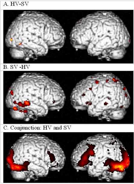
1. HV minus SV.
2. SV minus HV
3. Conjunction analysis of HV and SV

Choosing Regions of Interest and Preprocessing for Modeling

Regions of interest were chosen from the left ventral visual pathway in the words condition in our previous study (Tagamets et al., 2000). The rationale for choosing these regions is that they constitute the ventral visual pathway, and were all left lateralized for words in our previous study. The selected regions include area V1, V2, V4, inferior temporal (IT), inferior prefrontal cortex (PFC), and hippocampus The specific coordinates were selected from regional peaks in the conjunction analysis in the current study (Figure 4C), which reflects regions that are similarly active in both the HV and SV. For each region, the highest value in the region on the left determines the coordinate, and the ROI from the contralateral side is chosen as the peak within a 10 mm. radius of the corresponding left-sided coordinate (see Table 2 for the list of coordinates). Although we did not constrain the locations to be near our previously reported results, the maximum distance between the coordinates chosen above and regional maxima that we reported earlier is 10 mm. The ventral, as opposed to dorsal, inferior frontal gyrus (IFG) was chosen for its specificity to words in a previous connectivity analysis on this task (Bokde et al., 2001). In that analysis, performed with the same group of subjects as reported in Tagamets et. al., 2000, the finding was that ventral IFG was correlated with activity in left temporal regions only in the real words condition. Thus we hypothesized that a language-specific disconnection in schizophrenia is more likely to be found with this region.

Table 2.

Target values for regions in the ventral visual pathway. For each group, all activations are scaled to the left V1/V2 region in both the data and the model.

	Coordinates			LEFT Activity		RIGHT Activity
Region	X	Y	Z	HV	SV	HV	SV
V1/V2	−10	−100	−4	1.000	1.000	0.947	0.896
V4	−32	−88	−14	0.938	0.973	0.925	1.020
TEO/IT	−48	−64	−16	1.044	1.022	0.986	1.040
PFC	−50	34	−16	0.929	0.893	0.867	0.931
Hippocampus	−22	−22	−12	0.849	0.871	0.809	0.827

Before data is directly compared to the model, the data is extracted from the regions of interest (ROIs) and preprocessed to remove regional and global baseline effects. Regional variations in the baseline activity of the NMR signal are still poorly understood, and presumably are the product of processes that are not relevant to the state or task that is typically of interest in fMRI studies. A global signal has to be removed because the fMRI method does not yield absolute BOLD levels. Rather, for technical reasons, fMRI activity is relative, and varies from session to session and run to run. While the SPM analysis accounts for both regional and global effects, our goal is to model a single condition, and thus these effects need to be explicitly dealt with in preparing the data for modeling.

From the SPM-analyzed data, we extract a time series within each of five ROIs on each side of the brain, and these correspond to the regions included in the model. Each point in the time series is represented by the average over all voxels in a 4-mm radius ROI. The locations of these regions are given in Table 2. In order to account for differences in regional base activity levels, the extracted time series in each ROI is normalized to a common mean over the entire run. A mean within-condition value is then computed for each ROI by averaging over the series only within word condition blocks. A hemodynamic delay is accounted for by shifting the beginning points of task blocks by 6 seconds before averaging. Periods of transitions between blocks of different tasks can also skew the results. In order to ensure that activity was averaged during a steady-state task condition, the first two and the last two values from each block were not included in the average. Because the model does not include baseline signal, a 99% global baseline is computed over all ROIs and all conditions, and this is subtracted from the data. The lateral geniculate nucleus (LGN) is the source of input in the model, and is not modeled explicitly (see Tagamets 1998). Therefore, data for the LGN is not included among the fMRI ROIs, and in both the model and the data, the LGN activity is assumed to be equal in both hemispheres. The first entry point in which we have both modeled and experimental data to match is the V1/V2 region. Because the modeled synaptic activity is in arbitrary units, in order to be able to compare the modeled to the experimental data, we normalize all data, both modeled and experimental, to the left V1/V2 in each group.

In the following, we examine the within-task HV and SV data from the words condition. The preprocessed ROI data are given in Table 2. While activity in areas V4, TEO/IT and PFC tends to be left-lateralized in normal subjects, the schizophrenic patients display the opposite pattern in these regions (see Table 2).

Data-driven gains learning of inter-regional connections

In order to estimate the connection weights for each group, two identical instantiations of the model were initialized with identical random weights. Gains learning was applied to each instantiation of the model to fit the HV data and the SV data, respectively.

Gains learning was applied in two phases. In the first phase, gains learning was applied as described above. When the average error for each region dropped below 2%, the learning method was altered slightly. The regularization term is removed and then learning continues until the error drops below 1%. This second phase acts as fine-tuning what the first phase produces; it tends to take little time, and the gains are not changed substantially. It is necessary to have this second phase because the regularization term, while it will produce a unique solution in cases where multiple solutions would be possible otherwise, also inflates the average error. This is because once the learning begins to converge to gains that produce the correct activities on average region by region, the regularization tends to push this result away from what would be an optimal solution. Yet by doing the learning with regularization first, the ratios between weights are established and preserved when learning no longer includes regularization for the brief phase for fine-tuning.

Table 3 shows the results. After learning, the largest difference between average experimental and average modeled activations in any region was 0.96% for the HV group and 0.97% for the SV group, and the learning curves suggested that the gains algorithm had converged. Most connections are fairly similar between the groups. A notable exception is the significant difference between groups in the prefrontal-temporal connections in both hemispheres, with a reduction on the left side and an increase on the right in the SV relative to the HV. Left-sided fronto-temporal disconnection has been noted in a number of imaging studies of with language paradigms in schizophrenia (Fletcher et al., 1999; Lawrie et al., 2002). Our results also suggest a possibly compensatory increase in the corresponding right-sided temporo-fontal connections.

Table 3.

Weights learned by the model for healthy volunteers (HV) and volunteers with schizophrenia (SV). In order to account for potential scaling differences, connection weights from left LGN to V1 are fixed. Thus, other weights are relative to this connection.

		LEFT		RIGHT
Source	Destination	HV	SV	HV	SV
LGNs	V1/V2	0.141	0.141	0.129	0.124
V1/V2	V4	0.111	0.123	0.113	0.150
V4	TEO/IT	0.130	0.118	0.122	0.122
TEO/IT	PFC	0.058	0.015	0.033	0.066
TEO/IT	Hippocampus	0.079	0.087	0.080	0.076
Hippocampus	PFC	0.084	0.088	0.065	0.068

Model Accuracy and Dynamics after Gains Learning

We measured the accuracy of the model in its performance in the one-back matching task after gains learning was used to derive functional connectivity strengths that explain the data from the healthy volunteers. Performance of the model was then tested by presenting 16 trials, out of which four were matches. Accuracy on this task, as reflected by the decision units, is 100%.

Note that gains learning does not alter the coding properties of the individual units in any of the regions. These were established with the Hebbian learning rule. After gains learning, the dynamics of the units in the working memory circuit actually improved when compared to the original connection strengths, which were estimated by hand (Tagamets & Horwitz, 1998). Figure 5 shows the summed neural (electrical) activity of the different types of units in the WM circuit, using the original weights (5A) and after gains learning to the healthy volunteers' data (5B), and after gains learning on the data from the group with schizophrenia (5C). With the original weights, there was more saturation of activity in the D2 units, as evidenced by the sharp rise of activity to a plateau early in the cue period. As a consequence, the D1 units had a shorter delay period activity, though the response (decision to a match) was strong. The dynamics based on the SV are very similar to that from the HV. This demonstrates the robustness of the WM circuit, a property that is generally desirable in biological systems. The TEO/IT-to-PFC connections after gains learning on the HV data are about 50% of those in the original model, while these connections in the SV model are about 30% of the HV model, i.e. about 14% of the value in the original model. Despite these differences, all three versions display similar dynamics. When correlations among regions are computed from the fMRI data directly, all are much lower in the SV than in the HV, but the connection between left TEO/IT and PFC regions has the biggest difference, supporting the results from the gains learning.

Clearly, if gains are adjusted sufficiently high, behavior will degrade due to saturation of activity in all units. Conversely, if gains are too low, activity will not propagate or be sustained in the network. However, these results suggest that at least for the data from the current study, there is a range of possible inter-regional connection values for which the WM circuit performs correctly.

In the next section, we examine how local circuit changes in the PFC region can affect both the dynamics of the WM circuit and functional connectivity. In schizophrenia, synaptic density is thought to be reduced in frontal cortex (Benes et al., 1991; Selemon et al., 1998; Selemon & Goldman-Rakic, 1999; Benes, 2000), while evidence for compromised inter-regional white-matter tracts is either lacking or inconsistent (McGuire & Frith, 1996).

Effects of Local Circuits

We now examine whether modifying local circuitry can explain the data. Among other possibilities, abnormal activation in a region could come either from aberrant inputs from other regions or by disruptions in local circuits. In addition to the integrity of white-matter tracts between regions, we hypothesize that changes in local circuitry can play a significant role in apparent functional disconnection between regions. The relationship between structural and functional inter-regional connections is not necessarily straightforward. Although functional connectivity can reveal interactions in task-specific networks, the mechanisms that influence functional connectivity are poorly understood. In addition to structural inter-regional connections, other factors such as local circuitry, synaptic density, properties of neurotransmission, and neuromodulatory processes can affect functional connectivity. For example, one study suggests that integrity of local circuits, as measured by N-acetyl-aspartate (NAA), may play a substantial role in functional connectivity even when white matter tracts are intact in schizophrenia (Steel et al., 2001). Because the BOLD signal in fMRI is thought to mainly reflect synaptic activity (Jueptner & Weiller, 1995; Logothetis et al., 2001; Kim, 2003), and because most synapses in the brain arise locally (Gilbert & Wiesel, 1985; Douglas et al., 1995), it would be reasonable to assume that the local circuits can play a significant role in functional connectivity.

The working memory circuit in the model (see Figure 2B) implements delay period activity by recurrent connections between the two types of delay units, D1 and D2. D2 units become active when a stimulus is present and they maintain this activity during the delay period. The D1 units are not active during the stimulus presentation, but increase to a higher level of activity during the delay period only. Each of these unit types also has recurrent excitation to its own type of units, and this recurrence is important for maintenance of delay period activity. The goal is to examine how changing the self-recurrence of these units affects delay period activity, modeled BOLD signal, and functional connectivity with area TEO/IT. We hypothesized that relatively small changes in recurrence can disproportionately reduce measures of interregional functional connectivity, but reduce activation in PFC to a much lesser degree as long as the delay period activity is existent.

Effects of changing circuits in PFC

For each value w_R of recurrent excitation, simulations are run with sixteen trials of the delayed match-to-sample task. The summed synaptic activity is saved over each 200-iteration interval, which corresponds to about one second in time. Mean BOLD activation is computed as the total summed synaptic activity over all sixteen trials. In order to compute correlations between TEO/IT and PFC, it is necessary to account for the convolution of the BOLD response with the summed synaptic activity. The modeled synaptic activity is convolved with a Poisson function that has a peak at five seconds. Correlation coefficients between IT and PFC activations are then computed from their respective convolved time series.

Here we note that convolutions of the modeled synaptic activity is not necessary when averaging activations over a period of time, such as was done earlier when the goal was to match average activations. An extended period of time during which the same condition persists models an equilibrium state, during which convolution makes no difference, since the steady-state convolved activity is the summed activity times the area under the curve of the convolution function. By a well-known property of convolution, the area of the curve under two convolved functions equals the product of their areas:

$$\int {\mathrm{f}}^{\ast }\mathrm{g}=\int \mathrm{f}\mathrm{x}\int \mathrm{g}$$

Since the Poisson function we use is normalized to have an area of one, i.e. ∫ f = 1, the mean of the convolved function is equal to the mean of the original function. In contrast, computing correlations depends on the TR to TR changes. In this case the smoothing that is induced by the convolution becomes important when comparing experimental data to modeled data. For this reason, we convolve the modeled times series of synaptic activity before computing correlations from modeled data.

The working memory circuit displayed delay period activity for all values of D1 recurrence equal to or greater than w_D1 = 0.575. At values beyond w_D1 = 0.62, however, this activity tended to persist even after a decision had been made, possibly reflecting a mechanism for perseveration. The pattern of changes in modeled BOLD activation was different in regions PFC and TEO/IT, and within PFC, effects are different for changes to the D1 vs. the D2 units. In the PFC (Figure 6A), increasing the recurrence of either D1 or D2 units resulted in monotonically increasing activations in PFC, though the effects in D1 are more pronounced. The D1 units have increased activity only during the delay period, whereas D2 units have high activity both when stimuli are present and during the delay. In area TEO/IT, changes in BOLD that resulted from lowered recurrence in D1 and D2 units in PFC were smaller than changes in PFC, but they were non-monotonic (see Figure 6B). Furthermore, the effects of prefrontal D1 and D2 recurrence have opposing effects in area TEO/IT. Figure 6C shows how increasing recurrence in D1 and D2 units affects functional connectivity between regions TEO/IT and PFC. For each value of recurrence strength, correlations (r-values) are computed between modeled activities in the two regions. Again, the relationship is strongly non-monotonic, and relative changes to connectivity are much greater than changes to activations. Figure 6D shows the convolved model BOLD responses in areas TEO/IT and PFC over an extended time (about 35 seconds), when w_D1 = 0.575. There are nine trials during this period, with two stimuli per trial.

Figure 6.

Modeled BOLD and correlations between TEO/IT and PFC versus changing recurrence in PFC delay units. Self-recurrence from each unit (D1 or D2) to itself was varied from 0.57 to 0.63.

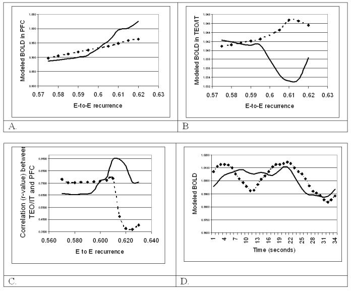
1. Modeled BOLD in PFC vs. recurrence in D1 and D2 units. Dotted line: D1 self-recurrence; Solid line: D2 self-recurrence; x-axis: amount of excitatory recurrence from the unit to itself, y-axis: modeled BOLD in PFC.
2. BOLD in area TEO/IT vs. recurrence in D1 and D2 units. Dotted line: D1 self-recurrence; Solid line: D2 self-recurrence; x-axis: amount of excitatory recurrence from the unit to itself, y-axis: Modeled BOLD in area TEO/IT.
3. Correlations between TEO/IT and PFC vs. recurrence of D1 or D2 units in area PFC. Dotted line: D1 self-recurrence; Solid line: D2 self-recurrence. x-axis: amount of excitatory recurrence from the unit to itself, y-axis: correlation coefficient (r-value) of activity between regions TEO/IT and PFC.
4. Modeled BOLD (convolved) when D1-to-D1 recurrent excitation equals = 0.575. Dotted line: BOLD activity in area TEO/IT; Solid line: BOLD activity in PFC. x-axis: Time (in seconds). Y-axis: Modeled BOLD activity.

Figure 7 shows the dynamics of the working memory circuit before and after reducing the connectivity when the local circuit recurrence is reduced to 0.575 from 0.6 in the D2 units. The main difference is that the delay period activity of the D1 units is shorter, due to a drop immediately after the second stimulus appears. This may explain a greater susceptibility to interference during working memory tasks in schizophrenia.

Figure 7.

Comparisons of WM circuit dynamics with and without reductions in local circuit recurrence.

1. Intact local circuits, trained with gains learning on the data from the schizophrenia group.
2. Local circuit recurrence reduced to 0.575 from 0.6 in the D2 units. The main difference is that the delay period activity of the D1 units is shorter, due to a drop immediately after the second stimulus appears. This may explain a greater susceptibility to interference during working memory tasks

In summary, the modeling results suggest that the configuration of local circuits can have a significant effect on functional connectivity between regions, while the effect on activations is relatively less dramatic. In the model, WM performance, as measured by the dynamics of the circuit in the PFC of the model, is more sensitive to disruptions of local recurrence than to changes in inter-regional connection strengths. Although WM performance was sustained for a range of values of local recurrence, this range is nowhere near the six-fold difference in inter-regional connections for which we demonstrated intact performance in the previous section. Taken together, the anatomical evidence and our modeling results suggest compromised local circuits may underlie the frequently observed functional disconnection between frontal and temporal cortex in schizophrenia.

The factors that underlie functional connectivity in human imaging studies are still poorly understood. In particular, functional and effective connectivity are often interpreted as reflecting the structural or physico-chemical connection strength between regions. The current modeling studies suggest that relatively moderate changes in local circuits can be reflected as disproportionately large changes in functional connectivity even when the connections between regions do not change. Although preliminary, our results suggest that this type of modeling approach can help elucidate underlying mechanisms from fMRI data to a greater extent than currently is possible.

Discussion

We have developed a large-scale systems-level model of regions in both cerebral hemispheres and an approach to examining potential underlying mechanisms for fMRI data. The model includes an algorithm that can be used to find effective strengths of interregional connectivity from an arbitrary data set. The inclusion of this gains learning method allows the model to generate plausible results for the pathways when trained on targets generated from brain imaging data. After demonstrating the performance of this algorithm on data with known connectivity, we applied it to an fMRI data set in order to examine differences between healthy control subjects and persons with schizophrenia. We found differences in temporo-frontal connections between the groups, a result that is consistent with a number of other imaging results in schizophrenia. Our results are characterized by a reduction in left-sided temporo-frontal connections and a concomitant increase on the right side, possibly due to compensatory mechanisms. Finally, we examined the effects of modifications in local prefrontal circuitry on changes in fMRI activations and functional connectivity. Our results suggest that functional connections are much more sensitive to these changes than BOLD activations. They further suggest the possibility that both reduced performance in working memory in schizophrenia and the functional disconnection between frontal and posterior regions in this disease may be explained by compromised local circuits.

The gains learning algorithm is a gradient descent method, which attempts to find solutions that will minimize the overall error between modeled and target activations. Two issues that need to be addressed for any learning rule are its convergence and uniqueness. Convergent behavior in a system guarantees that some solution will be found. Uniqueness means that there is only one solution, thus guaranteeing that if the system exhibits convergence, different initial conditions will all lead to the same final solution. Because of the complexity of the activation equations involved in the model, which depend on time, previous states, and the highly nonlinear effect of the local circuitry, a formal analysis of the convergence and uniqueness of the explicit model over the course of training has not been feasible. Although convergence and uniqueness cannot be proven, empirical evidence over multiple simulations with different initial conditions and known connections suggests both convergence and uniqueness of the gains learning method. We addressed this by running the learning algorithm from a variety of starting conditions and examining the similarity and correctness of the final solutions.

In our current models, we make the assumption that fMRI activity mainly reflects local synaptic activity in a region, and includes both afferents from other regions and local circuitry. This view is still generally held to be true (Magistretti & Pellerin, 1999; Logothetis et al., 2001). The issue of how to translate baseline and scaling effects in fMRI is still poorly understood. A baseline NMR signal that is unrelated to neural activity is always present in the brain. It has been estimated that this baseline signal accounts for most of the signal in fMRI, and a typical fMRI signal in a subtraction design is on the order of one percent of total signal (Gusnard et al., 2001). As a preliminary approach, we dealt with this issue by subtracting 99% of the average signal from the experimental data, thus leaving only the portion that can be attributed to changes in neuronal processing. Scaling differences, both global and regional, are also a potential confound when examining within-condition activity in fMRI. The fMRI signal is not an absolute measure of anything, and can even drift during a single run over a period of a few minutes. Such short-term drift is generally dealt with by using high-pass filters during data analysis. Filtering is not an option for dealing with longer-term instability in the signal, such as across different runs, different sessions, or different days. Rather, this is usually dealt with by including at least two conditions in any run and analyzing data by contrasting these conditions to each other. In order to relate within-condition, non-contrast, modeled to experimental data, both of which are in arbitrary units, we chose to use the left early visual cortex as an “anchor”, so that all other regional activations in the model are relative to this. Although this region also fluctuates with the task, it is one of the few brain regions that has not been found to be abnormal in schizophrenia. Thus, all of the results are relative to this region in each group. Finally, there are substantial differences in baseline signal in different regions of the brain. The reasons for this are poorly understood. We approached this problem by scaling all regional time series to a common mean value. Rather than try to model these poorly understood phenomena, we pre-treated the data with the intent of eliminating as many of these effects as possible, with the goal that both the model and fMRI data are as pure measures of neural activity as possible. As more is learned about these factors, they can be better dealt with in future modeling efforts.

Here we examined the nature of the visual processing aspects of the word stimuli, and have not taken account of the linguistic content of these stimuli. The goal of the current study is to examine the nature of previously reported functional disconnection between frontal and temporal regions that has been observed in schizophrenia, as well as in our own work. We have previously suggested that the familiarity of words as whole visual objects may have a significant effect on the activation patterns, and our previous results suggested that in this task, words and non-word strings involve the same basic circuits in the left ventral visual pathway (Tagamets et al., 2000). In the future, it would be beneficial to extend the model to include processes that are specific to language. However, the current knowledge of the neural underpinnings of this function is rudimentary.

Virtually all current methods of fMRI data analysis are descriptive. Interpretation is left to individual investigators, who are faced with enormous challenges in trying to fit a highly complex dynamical system into a theory that can be explained by a few blobs. The goal of our modeling efforts has been to increase understanding of possible interactions between underlying mechanisms and the results that are observed in imaging data. We expect that as knowledge about these mechanisms increases, it will be incorporated into models such as this, and that these models can be integrated into current data analysis methods in order to enrich understanding of what is happening “under the hood”.

We believe that this type of approach is very useful in order to optimize the usefulness and application of the vast amount of current knowledge of underlying mechanisms in the brain to a better understanding of human imaging data. We have taken a number of steps to adhere to principles rather than specific instances of data, and to constrain the number of free parameters. One primary goal has been to include flexibility in design that easily allows extensions as new data becomes available. The basis for assigning parameter values is not to fit the data, but rather they are chosen a priori from data and existing theoretical knowledge. In this framework, constraints from physiology are used wherever this data is available. For example, the connectivity of the basic local circuit was computed from physiological data, and once this was done, these values are fixed for all regions of the model. If directly quantifiable values are not available, the choices for values of parameters are based on principles derived from the biological data. For example, interregional connections are specified by three parameters that capture principles of connectivity rather than specific configurations: total weight, fanout size (extent), and sparseness. These parameters are quantifiable from biological data, but in large part specific values are unknown. In our model, the original total weights from LGN to V1/V2, from V1/V2 to V4, and V4 to IT in the model are based on reported values for these connections in the literature (see Tagamets et. al, 1998 for details). Fanouts of connections between regions are based on data that suggest a three-fold increase in receptive field size at each stage along the ventral visual pathway (Desimone et al., 1984). We conclude that this combined theory-driven and data-driven methodology extends current imaging analysis methods and allows examination of properties other than total activations and functional interregional connection strengths.

References

- Ackermann RF, Finch DM, Babb TL, Engel J., Jr. Increased glucose metabolism during long-duration recurrent inhibition of hippocampal pyramidal cells. Journal of Neuroscience. 1984;4:251–264. doi: 10.1523/JNEUROSCI.04-01-00251.1984. [DOI] [PMC free article] [PubMed] [Google Scholar]
- Arbib MA, Bischoff A, Fagg AH, Grafton ST. Synthetic PET: Analyzing large-scale properties of neural networks. Human Brain Mapping. 1995;2:225–233. [Google Scholar]
- Arfanakis K, Cordes D, Haughton VM, Moritz CH, Quigley MA, Meyerand ME. Combining independent component analysis and correlation analysis to probe interregional connectivity in fMRI task activation datasets. Magn Reson.Imaging. 2000;18:921–930. doi: 10.1016/s0730-725x(00)00190-9. [DOI] [PubMed] [Google Scholar]
- Artiges E, Martinot JL, Verdys M, Attar-Levy D, Mazoyer B, Tzourio N, Giraud MJ, Paillere-Martinot ML. Altered hemispheric functional dominance during word generation in negative schizophrenia. Schizophrenia Bulletin. 2000;26:709–721. doi: 10.1093/oxfordjournals.schbul.a033488. [DOI] [PubMed] [Google Scholar]
- Benes FM. Emerging principles of altered neural circuitry in schizophrenia. Brain Res.Brain Res.Rev. 2000;31:251–269. doi: 10.1016/s0165-0173(99)00041-7. [DOI] [PubMed] [Google Scholar]
- Benes FM, McSparren J, Bird ED, SanGiovanni JP, Vincent SL. Deficits in small interneurons in prefrontal and cingulate cortices of schizophrenic and schizoaffective patients. Arch.Gen.Psychiatry. 1991;48:996–1001. doi: 10.1001/archpsyc.1991.01810350036005. [DOI] [PubMed] [Google Scholar]
- Bokde AL, Tagamets MA, Friedman RB, Horwitz B. Functional interactions of the inferior frontal cortex during the processing of words and word-like stimuli. Neuron. 2001;30:609–617. doi: 10.1016/s0896-6273(01)00288-4. [DOI] [PubMed] [Google Scholar]
- Brincat SL, Connor CE. Underlying principles of visual shape selectivity in posterior inferotemporal cortex. Nat.Neurosci. 2004;7:880–886. doi: 10.1038/nn1278. [DOI] [PubMed] [Google Scholar]
- Caesar K, Gold L, Lauritzen M. Context sensitivity of activity-dependent increases in cerebral blood flow. Proceedings of the National Academy of Sciences-USA. 2003;100:4239–4244. doi: 10.1073/pnas.0635075100. [DOI] [PMC free article] [PubMed] [Google Scholar]
- Calhoun VD, Adali T, Kiehl KA, Astur R, Pekar JJ, Pearlson GD. A method for multitask fMRI data fusion applied to schizophrenia. Hum.Brain Mapp. 2005 doi: 10.1002/hbm.20204. [DOI] [PMC free article] [PubMed] [Google Scholar]
- Calhoun VD, Adali T, McGinty VB, Pekar JJ, Watson TD, Pearlson GD. fMRI activation in a visual-perception task: network of areas detected using the general linear model and independent components analysis. Neuroimage. 2001;14:1080–1088. doi: 10.1006/nimg.2001.0921. [DOI] [PubMed] [Google Scholar]
- Corchs S, Deco G. Large-scale neural model for visual attention: integration of experimental single-cell and fMRI data. Cereb.Cortex. 2002;12:339–348. doi: 10.1093/cercor/12.4.339. [DOI] [PubMed] [Google Scholar]
- Corchs S, Deco G. Feature-based attention in human visual cortex: simulation of fMRI data. NeuroImage. 2004;21:36–45. doi: 10.1016/j.neuroimage.2003.08.045. [DOI] [PubMed] [Google Scholar]
- Cordes D, Haughton VM, Arfanakis K, Wendt GJ, Turski PA, Moritz CH, Quigley MA, Meyerand ME. Mapping functionally related regions of brain with functional connectivity MR imaging. AJNR Am.J.Neuroradiol. 2000;21:1636–1644. [PMC free article] [PubMed] [Google Scholar]
- Desimone R, Albright TD, Gross CG, Bruce C. Stimulus-selective properties of inferior temporal neurons in the macaque. Journal of Neuroscience. 1984;4:2051–2062. doi: 10.1523/JNEUROSCI.04-08-02051.1984. [DOI] [PMC free article] [PubMed] [Google Scholar]
- Desimone R, Schein SJ, Moran J, Ungerleider LG. Contour, color and shape analysis beyond the striate cortex. Vision Res. 1985;25:441–452. doi: 10.1016/0042-6989(85)90069-0. [DOI] [PubMed] [Google Scholar]
- Dolan RJ, Fletcher P, Frith CD, Friston KJ, Frackowiak RS, Grasby PM. Dopaminergic modulation of impaired cognitive activation in the anterior cingulate cortex in schizophrenia. Nature. 1995;378:180–182. doi: 10.1038/378180a0. [DOI] [PubMed] [Google Scholar]
- Douglas RJ, Koch C, Mahowald M, Martin KA, Suarez HH. Recurrent excitation in neocortical circuits. Science. 1995;269:981–985. doi: 10.1126/science.7638624. [DOI] [PubMed] [Google Scholar]
- Fletcher P, McKenna PJ, Friston KJ, Frith CD, Dolan RJ. Abnormal cingulate modulation of fronto-temporal connectivity in schizophrenia. NeuroImage. 1999;9:337–342. doi: 10.1006/nimg.1998.0411. [DOI] [PubMed] [Google Scholar]
- Fletcher PC, Frith CD, Grasby PM, Friston KJ, Dolan RJ. Local and distributed effects of apomorphine on fronto-temporal function in acute unmedicated schizophrenia. Journal of Neuroscience. 1996;16:7055–7062. doi: 10.1523/JNEUROSCI.16-21-07055.1996. [DOI] [PMC free article] [PubMed] [Google Scholar]
- Friston KJ, Ashburner J, Frith CD, Poline JB, Heather JD, Frackowiak RSJ. Spatial registration and normalization of images. Human Brain Mapping. 1995a;3:165–189. [Google Scholar]
- Friston KJ, Harrison L, Penny W. Dynamic causal modelling. NeuroImage. 2003;19:1273–1302. doi: 10.1016/s1053-8119(03)00202-7. [DOI] [PubMed] [Google Scholar]
- Friston KJ, Holmes AP, Worsley KJ, Poline JP, Frith CD, Frackowiak RSJ. Statistical parametric maps in functional imaging: A general linear approach. Human Brain Mapping. 1995b;2:189–210. [Google Scholar]
- Funahashi S, Bruce C, Goldman-Rakic PS. Visuospatial coding in primate prefrontal neurons revealed by oculomotor paradigms. Journal of Neurophysiology. 1990;63:814–831. doi: 10.1152/jn.1990.63.4.814. [DOI] [PubMed] [Google Scholar]
- Gilbert CD, Wiesel TN. Intrinsic connectivity and receptive field properties in visual cortex. Vision Res. 1985;25:365–374. doi: 10.1016/0042-6989(85)90061-6. [DOI] [PubMed] [Google Scholar]
- Girosi F, Jones M, Poggio T. Regularization Theory and Neural Networks Architectures. Neural Comput. 1995;7:219–269. [Google Scholar]
- Glantz LA, Lewis DA. Decreased dendritic spine density on prefrontal cortical pyramidal neurons in schizophrenia. Arch.Gen.Psychiatry. 2000;57:65–73. doi: 10.1001/archpsyc.57.1.65. [DOI] [PubMed] [Google Scholar]
- Goldman-Rakic PS. Cellular basis of working memory. Neuron. 1995;14:477–485. doi: 10.1016/0896-6273(95)90304-6. [DOI] [PubMed] [Google Scholar]
- Gusnard DA, Raichle ME, Raichle ME. Searching for a baseline: functional imaging and the resting human brain. Nat.Rev.Neurosci. 2001;2:685–694. doi: 10.1038/35094500. [DOI] [PubMed] [Google Scholar]
- Horwitz B, Sporns O. Neural modeling and functional neuroimaging. Human Brain Mapping. 1994;1:269–283. doi: 10.1002/hbm.460010405. [DOI] [PubMed] [Google Scholar]
- Horwitz B, Long TW, Tagamets MA. The neurobiological substrate of PET-fMRI functional connectivity. NeuroImage. 1999;9:S392. [Google Scholar]
- Horwitz B, Warner B, Fitzer J, Tagamets MA, Husain FT, Long TW. Investigating the neural basis for functional and effective connectivity. Application to fMRI. Proceedings of the Royal Society of London B, Philosophical Transactions: Biology. 2005;360:1108–2970. doi: 10.1098/rstb.2005.1647. [DOI] [PMC free article] [PubMed] [Google Scholar]
- Jueptner M, Weiller C. Review: Does measurement of regional cerebral blood flow reflect synaptic activity?--Implications for PET and fMRI. NeuroImage. 1995;2:148–156. doi: 10.1006/nimg.1995.1017. [DOI] [PubMed] [Google Scholar]
- Kim SG. Progress in understanding functional imaging signals. Proceedings of the National Academy of Sciences - USA. 2003;100:3550–3552. doi: 10.1073/pnas.0730809100. [DOI] [PMC free article] [PubMed] [Google Scholar]
- Kircher TT, Liddle PF, Brammer MJ, Williams SC, Murray RM, McGuire PK. Reversed lateralization of temporal activation during speech production in thought disordered patients with schizophrenia. Psychol.Med. 2002;32:439–449. doi: 10.1017/s0033291702005287. [DOI] [PubMed] [Google Scholar]
- Kolluri N, Sun Z, Sampson AR, Lewis DA. Lamina-specific reductions in dendritic spine density in the prefrontal cortex of subjects with schizophrenia. Am.J.Psychiatry. 2005;162:1200–1202. doi: 10.1176/appi.ajp.162.6.1200. [DOI] [PubMed] [Google Scholar]
- Lawrie SM, Buechel C, Whalley HC, Frith CD, Friston KJ, Johnstone EC. Reduced frontotemporal functional connectivity in schizophrenia associated with auditory hallucinations. Biological Psychiatry. 2002;51:1008–1011. doi: 10.1016/s0006-3223(02)01316-1. [DOI] [PubMed] [Google Scholar]
- Lewis DA, Gonzalez-Burgos G. Intrinsic excitatory connections in the prefrontal cortex and the pathophysiology of schizophrenia. Brain Res.Bull. 2000;52:309–317. doi: 10.1016/s0361-9230(99)00243-9. [DOI] [PubMed] [Google Scholar]
- Logothetis NK, Pauls J, Augath M, Trinath T, Oeltermann A. Neurophysiological investigation of the basis of the fMRI signal. Nature. 2001;412:150–157. doi: 10.1038/35084005. [DOI] [PubMed] [Google Scholar]
- Magistretti PJ, Pellerin L. Cellular mechanisms of brain energy metabolism and their relevance to functional brain imaging. Philos.Trans.R.Soc.Lond B Biol.Sci. 1999;354:1155–1163. doi: 10.1098/rstb.1999.0471. [DOI] [PMC free article] [PubMed] [Google Scholar]
- McGuire PK, Frith CD. Disordered functional connectivity in schizophrenia. Psychol.Med. 1996;26:663–667. doi: 10.1017/s0033291700037673. [DOI] [PubMed] [Google Scholar]
- McIntosh AR. Understanding neural interactions in learning and memory using functional neuroimaging. Ann.N.Y.Acad.Sci. 1998;855:556–571. doi: 10.1111/j.1749-6632.1998.tb10625.x. [DOI] [PubMed] [Google Scholar]
- McIntosh AR, Chau WK, Protzner AB. Spatiotemporal analysis of event-related fMRI data using partial least squares. NeuroImage. 2004;23:764–775. doi: 10.1016/j.neuroimage.2004.05.018. [DOI] [PubMed] [Google Scholar]
- McIntosh AR, Gonzalez-Lima F. The application of structiral equation modeling to metabolic mapping of functional neural systems. In: Gonzalez-Lima F, et al., editors. Advances in metabolic mapping techniques for brain imaging of behavioral and learning functions. Kluwer Academic Publishers; Netherlands: 1992. pp. 219–255. [Google Scholar]
- McIntosh AR, Gonzalez-Lima F. Structural equation modeling and its applicaton to network analysis in functional brain imaging. Human Brain Mapping. 1994;2:2–22. [Google Scholar]
- McIntosh AR, Lobaugh NJ. Partial least squares analysis of neuroimaging data: applications and advances. NeuroImage. 2004;23(Suppl 1):S250–S263. doi: 10.1016/j.neuroimage.2004.07.020. [DOI] [PubMed] [Google Scholar]
- Mechelli A, Price CJ, Noppeney U, Friston KJ. A dynamic causal modeling study on category effects: bottom-up or top-down mediation? J.Cogn Neurosci. 2003;15:925–934. doi: 10.1162/089892903770007317. [DOI] [PubMed] [Google Scholar]
- Penny WD, Stephan KE, Mechelli A, Friston KJ. Modelling functional integration: a comparison of structural equation and dynamic causal models. NeuroImage. 2004 doi: 10.1016/j.neuroimage.2004.07.041. [DOI] [PubMed] [Google Scholar]
- Poggio T, Torre V, Koch C. Computational vision and regularization theory. Nature. 1985;317:314–319. doi: 10.1038/317314a0. [DOI] [PubMed] [Google Scholar]
- Ragland JD, Gur RC, Valdez J, Turetsky BI, Elliott M, Kohler C, Siegel S, Kanes S, Gur RE. Event-related fMRI of frontotemporal activity during word encoding and recognition in schizophrenia. Am.J.Psychiatry. 2004;161:1004–1015. doi: 10.1176/appi.ajp.161.6.1004. [DOI] [PMC free article] [PubMed] [Google Scholar]
- Selemon LD, Goldman-Rakic PS. The reduced neuropil hypothesis: a circuit based model of schizophrenia. Biological Psychiatry. 1999;45:17–25. doi: 10.1016/s0006-3223(98)00281-9. [DOI] [PubMed] [Google Scholar]
- Selemon LD, Rajkowska G, Goldman-Rakic PS. Elevated neuronal density in prefrontal area 46 in brains from schizophrenic patients: application of a three-dimensional, stereologic counting method. J Comp Neurol. 1998;392:402–412. [PubMed] [Google Scholar]
- Sommer IE, Ramsey NF, Kahn RS. Language lateralization in schizophrenia, an fMRI study. Schizophr.Res. 2001;52:57–67. doi: 10.1016/s0920-9964(00)00180-8. [DOI] [PubMed] [Google Scholar]
- Steel RM, Bastin ME, McConnell S, Marshall I, Cunningham-Owens DG, Lawrie SM, Johnstone EC, Best JJ. Diffusion tensor imaging (DTI) and proton magnetic resonance spectroscopy (1H MRS) in schizophrenic subjects and normal controls. Psychiatry Res. 2001;106:161–170. doi: 10.1016/s0925-4927(01)00080-4. [DOI] [PubMed] [Google Scholar]
- Tagamets MA, Horwitz B. Interpreting PET and fMRI measures of functional neural activity: the effects of synaptic inhibition on cortical activation in human imaging studies. Brain Res.Bull. 2001;54:267–273. doi: 10.1016/s0361-9230(00)00435-4. [DOI] [PubMed] [Google Scholar]
- Tagamets MA, Horwitz B. Integrating electrophysiological and anatomical experimental data to create a large-scale model that simulates a delayed match-to-sample human brain imaging study. Cereb.Cortex. 1998;8:310–320. doi: 10.1093/cercor/8.4.310. [DOI] [PubMed] [Google Scholar]
- Tagamets MA, Horwitz B. A model of working memory: Bridging the gap between electrophysiology and human brain imaging. Neural Networks. 2000;13:941–952. doi: 10.1016/s0893-6080(00)00063-0. [DOI] [PubMed] [Google Scholar]
- Tagamets MA, Novick JM, Chalmers ML, Friedman RB. A parametric approach to orthographic processing in the brain: an fMRI study. J.Cogn Neurosci. 2000;12:281–297. doi: 10.1162/089892900562101. [DOI] [PubMed] [Google Scholar]
- Tagamets MA, O'Donnell PS, Cortes CR, Lahti AC, Holcomb HH, Tamminga CA. An fMRI study of orthographic familiarization in schizophrenia. Society for Neuroscience; Washington, D.C.: 2002. Program No. 705.5 ed. [Google Scholar]
- Tanaka K. Neuronal mechanisms of object recognition. Science. 1993;262:685–688. doi: 10.1126/science.8235589. [DOI] [PubMed] [Google Scholar]
- Tanaka K. Columns for complex visual object features in the inferotemporal cortex: clustering of cells with similar but slightly different stimulus selectivities. Cereb.Cortex. 2003;13:90–99. doi: 10.1093/cercor/13.1.90. [DOI] [PubMed] [Google Scholar]
- Wilson HR, Cowan JD. Excitatory and inhibitory interactions in localized populations of model neurons. Biophys.J. 1972;12:1–24. doi: 10.1016/S0006-3495(72)86068-5. [DOI] [PMC free article] [PubMed] [Google Scholar]