A Generalized Combinatorial Approach for Detecting Gene-by-Gene and Gene-by-Environment Interactions with Application to Nicotine Dependence

Abstract

The determination of gene-by-gene and gene-by-environment interactions has long been one of the greatest challenges in genetics. The traditional methods are typically inadequate because of the problem referred to as the “curse of dimensionality.” Recent combinatorial approaches, such as the multifactor dimensionality reduction (MDR) method, the combinatorial partitioning method, and the restricted partition method, have a straightforward correspondence to the concept of the phenotypic landscape that unifies biological, statistical genetics, and evolutionary theories. However, the existing approaches have several limitations, such as not allowing for covariates, that restrict their practical use. In this study, we report a generalized MDR (GMDR) method that permits adjustment for discrete and quantitative covariates and is applicable to both dichotomous and continuous phenotypes in various population-based study designs. Computer simulations indicated that the GMDR method has superior performance in its ability to identify epistatic loci, compared with current methods in the literature. We applied our proposed method to a genetics study of four genes that were reported to be associated with nicotine dependence and found significant joint action between CHRNB4 and NTRK2. Moreover, our example illustrates that the newly proposed GMDR approach can increase prediction ability, suggesting that its use is justified in practice. In summary, GMDR serves the purpose of identifying contributors to population variation better than do the other existing methods.

Most, if not all, phenotypic traits of biomedical relevance in humans and of economic importance in plants and animals are the result of a series of dynamic, interrelated, and hierarchical metabolic pathways under the control of jointly acting networks of genes and environmental factors.^1–5 When the change of a genetic factor or an alteration in environment perturbs the overall homeostasis of such a system, there may be detectable marginal effects on a phenotypically relevant outcome. When some factors approximately meet the criteria of conditional independence, as defined by Bayesian network theory, their marginal effects can be viewed as being independent of one another. This is the basic logic of traditional approaches that typically attempt to isolate one factor at a time and to ascribe the phenotype to some kind of additive or combinatorial effects of these factors. Such strategies, however, can fail to detect the determinants if their measured effects on variation depend on the context defined by other genes and/or by exposures to environments—that is, if there exist gene-by-gene interaction (epistasis) and/or gene-by-environment interaction (plastic reaction norms).^6,7

It has been well documented in the literature that, as natural properties of complex networks and the ubiquitous intermolecular dependence in gene regulation and biochemical and metabolic systems, joint actions are the norm rather than the exception in the inherited traits.^7–12 Traditional methods for detecting these as statistical interactions are usually established by an extension under the concept of single-factor–based approaches.¹³ Such methods, in which the total number of possible parameters could rapidly outpace the total size of any sample with increase in dimension, have several practical limitations, such as having a heavy computational burden (often being computationally intractable) and increased type I and II errors and being less robust and potentially biased as a result of highly sparse data in a multifactorial model. Thus, they are hardly appropriate for tackling elusive gene-gene and gene-environment interactions.

Recently, several approaches have emerged as promising tools for detecting gene-by-gene and gene-by-environment interactions in either dichotomous or continuous phenotypes. For example, Ritchie and her colleagues^14–16 proposed an algorithm, called the “multifactor dimensionality reduction” (MDR) method, for balanced case-control or discordant sib-pair designs. Hahn and Moore¹⁷ presented a mathematical proof that shows that MDR ideally discriminates between discrete clinical endpoints by the use of multilocus genotypes. Recently, Martin et al.¹⁸ extended the MDR method for family-based designs, and Velez et al.¹⁹ proposed a balanced accuracy function to detect interactions in unbalanced data sets.

Since publication of the original report,¹⁴ MDR has been applied by many research groups to detect interactions for a number of complex disorders (for a detailed list of publications, see the Epistasis Blog). However, there still exist several limitations in the currently established MDR implementation that may restrict its practical use in genetic data analysis: (1) it does not allow for adjustment of covariates such as ethnicity, sex, weight, and/or age, and (2) it is applicable only to dichotomous phenotypes, not to continuous phenotypes that contain more information.

Nelson et al.²⁰ developed the combinatorial partitioning method (CPM) for quantitative traits, which shares a similarity with the MDR method. Prohibitively intensive computation makes this method less practical for dealing with cases with more than two loci. Culverhouse et al.²¹ advocated the restricted partition method (RPM). Although it substantially reduces the computational burden, as compared with the CPM, the RPM still requires significant computational effort for high-dimensional data. Further, the validity of the RPM relies on a reasonably good partitioning of genotypes into subgroups implemented iteratively by multiple comparison tests.²² Moreover, neither Nelson et al.²⁰ nor Culverhouse et al.²¹ included covariates in their approaches.

In this article, we propose a generalized MDR (GMDR) framework based on the score of a generalized linear model, of which the original MDR method is a special case. Our proposed approach has several advantages: (1) it permits adjustment for covariates, (2) it provides a unified framework for coherently handling both dichotomous and quantitative phenotypes, and (3) it is applicable to a variety of flexible population-based study designs—for example, it can be applied without modification to unbalanced case-control samples and to both random and selected samples. To help readers follow our approach, we first present the theory and then demonstrate, through a series of simulations for both continuous and dichotomous phenotypes, the improvements it leads to in testing accuracy and cross-validation consistency when an informative covariate exists. Finally, we apply our proposed novel approach to a genetic data set on tobacco dependence and find significant joint action of genes for nicotine dependence (ND).

Methods

In this section, we first introduce the generalized linear model commonly used for either dichotomous or continuous phenotypes. We then introduce the concept of a score statistic into the current MDR framework and formulate our GMDR approach. We should emphasize that the score-based derivation should be considered merely a device for obtaining an appropriate statistic to classify multifactor cells into different two groups. It is not necessarily implied that the GMDR method is likelihood based; for example, we can use other measures computed via least-squares regression or other statistical methods for nonnormal continuous traits. Moreover, like MDR,¹⁶ the GMDR method can also be considered a constructive induction approach.

Models

Let y_i denote the phenotype of individual i, either dichotomous or continuous, with expectation E(y_i)=μ_i. In general, it can be represented by a generalized linear model in the exponential family of distributions that includes the normal, Poisson, and Bernoulli distributions^23,24:

where l(μ_i) is an appropriate link function, α is the intercept, x_i is the predictor-variable vector that codes gene-by-gene and/or gene-by-environment interactions of interest, z_i is the vector coding for covariates, and β and γ are the corresponding parameter vectors. In what follows, we call β the “target effects.” With dichotomous phenotypes following, say, a Bernoulli distribution, a natural link function is the logit,

For continuous phenotypes having a normal distribution, the natural link is the identity. In the presence of statistical interactions between the target attributes and covariates, the above model can be further extended to

where δ is the vector of the interaction effects and ⊗ represents a direct (Kronecker) product.

Score Statistics

The log-prospective likelihood of independent observations y_i and i=1,2,…,n, with conditioning on the predictor-variable vectors x_i and z_i, can be written as^23,24

where y is the vector of observations, Ω is the vector of parameters, Ω=(α,β,γ) in model (1) and Ω=(α,β,γ,δ) in model (2), and is a function of l(μ_i) with the property that when l(μ_i) is a canonical link function. The first partial derivative of the log-likelihood, also termed the “score,” is

where θ∈Ω. Setting β=0 in model (1) yields the residual score vector

where component , the estimated expectation is , and are the maximum-likelihood estimates (MLEs) under the null hypothesis H₀ (β=0) (i.e., no target effects of study), and is the contribution of individual i to the score for β_j. Likewise, we obtain the residual score vector for model (2) by setting β=0 and δ=0:

where component is analogous to that in equation (3), component

is the MLE under H₀ (β=0 and δ=0), and is the contribution of individual i to the score for δ_k.

Then, we define the following score-based statistics for individual i, on the basis of normalized contributions:

and

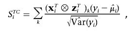
where is the estimated variance of y_i, and where S^T_i, S^TC_i, and S^T+TC_i, respectively, measure the normalized contributions to the scores of the target effects, target-by-covariate interactions, and both target and target-by-covariate effects. We can use any one of the three according to our purpose. We use S^T_i to illustrate our GMDR method, which we call the “score-based MDR” method for the time being.

Score-Based MDR Method

The score-based MDR method proposed in this article uses the same data-reduction strategy as does the original MDR method^14,15—that is, the possible cells classified by a set of factors are pooled into two distinct groups, effectively reducing the dimensionality from multidimensional to one-dimensional and thereby identifying, from all potential combinations, the specific combinations of factors that show the strongest association with the phenotype. To make the presentation self-contained, we first briefly review the current MDR procedure and then describe our generalization under the same framework, using the score statistic to define the two distinct groups. As shown below, the current MDR method is a specific case of our GMDR method.

Figure 1, adapted from the work of Ritchie et al.¹⁴ and Hahn et al.,¹⁵ illustrates the general steps involved in implementing the MDR method for case-control or discordant-sib studies. In the first step, the data are randomly split into some number of equal parts for cross-validation; for an illustrative purpose, the use of 10-fold cross-validation is shown in figure 1. One subdivision is used as the testing set and the rest as the independent training set. Then, steps 2–5 are run for the training set and step 6 for the testing set. (To reduce the fluctuations due to chance divisions of the data, each possible training set and its corresponding testing set are used, and the results are averaged. The consistency of the model across cross-validation training sets [i.e., how many times the same MDR model is identified in all the possible training sets] is also evaluated.) In the second step, a set of n genetic and/or discrete environmental factors is selected from the list of all factors. In the third step, the possible multifactor classes or cells defined by the n factors are represented in n-dimensional space. Then, the ratio of the number of cases to the number of controls is calculated within each multifactor cell. In the fourth step, each multifactor cell in n-dimensional space is labeled either as “high-risk” if the ratio of cases to controls meets or exceeds a preassigned threshold T (e.g., T=1), including the cells that have cases but no controls, as “low-risk” if the threshold is not exceeded, including the cells that have controls but no cases, or as “empty” otherwise. A model is formulated by pooling high-risk cells into one group and low-risk cells into another group. In the fifth step, all potential combinations of n factors are evaluated sequentially for their ability to classify cases and controls in the training data, and the best n-factor model that yields minimum misclassification error is chosen. In the sixth step, the independent testing set is used to estimate the prediction error of the best model selected from the fifth step. Finally, among this set of best models, we pick the model that has minimum prediction error and/or maximum cross-validation consistency.

Figure 1. .

Summary of the steps involved in implementing the MDR and GMDR methods (adapted from the work of Ritchie et al.¹⁴ and Hahn et al.¹⁵). The two methods share the same reduction strategy. The difference is that, in the GMDR method, we substitute a score statistic or some other quantitative measure, instead of affection status, to define the two different groups. In balanced case-control studies with no covariate, the two methods are exactly equivalent—that is, given an equivalent threshold, the two methods yield the same results, including the best model and classification and prediction accuracies. For a detailed description of the steps, please see the “Score-Based MDR Method” subsection. In step 3, bars represent hypothetical distributions of cases (left, dark shading) and controls (right, light shading); numbers not in parentheses above bars are the numbers of cases and controls, and those in parentheses are the sums of the scores. In steps 4 and 6, numbers not in parentheses are the ratios of the number of cases to the number of controls, and those in parentheses are the average scores. “High-risk” cells are indicated by dark shading, “low-risk” cells by light shading, and “empty” cells by no shading.

In our generalization, we replace the ratio of cases to controls by the score in each cell to discriminate between high-risk and low-risk cells and assess classification accuracy and prediction error, while keeping the rest of the procedure unchanged. First, we compute the MLEs and the score values of all individuals under the null hypothesis, H₀: β=0 for model (1) or β=0 and δ=0 for model (2). Since the null hypothesis assumes there are no effects of the putative factors or their interactions, the score values are the same for all different factor classifications. Now, in the third step, the cumulative score value is calculated within each multifactor cell. In the fourth step, each multifactor cell is labeled either as “high-risk” if the average score meets or exceeds a preassigned threshold T (e.g., 0) or as “low-risk” if the threshold is not exceeded. Correspondingly, we substitute the score values for the numbers of cases and controls, to evaluate the classification and prediction errors, and thereby identify the best model in later steps. The original MDR method is a specific version of the method proposed in this report. For balanced case-control studies with no covariates, the sample prevalence is . The case:control ratio within each cell is replaced by the cell’s average score—for example, 1:1 is equivalent to a score value 0.

This generalization offers much flexibility in the use of covariates, different study designs, and different types of phenotypes. The method allows for covariate adjustments and provides a unified framework for analyzing both continuous and dichotomous traits, as well as others, under generalized linear models. It can also be applied without modification to unbalanced case-control, random, and selected samples. Moreover, although we borrow the concept of score functions to formulate it, our GMDR method is not dependent on the usual score or likelihood properties. The validity of the GMDR method depends only on the availability of an appropriate statistic that can provide a measure of the association between the putative factors and the phenotype. Other statistics, such as moment and least-squares statistics, can also be used. Thus, like the MDR method, the GMDR method can be considered model free.

Results

Simulation Results

To evaluate the ability of the GMDR method to detect factor interactions, we simulated a series of data sets on a sample consisting of 1,000 unrelated subjects for both continuous and dichotomous phenotypes under three different epistatic models that have been considered before—that is, digenic, trigenic, and tetragenic interaction models—but each with one extra risk factor (covariate) that contributes to the phenotype. Genotypes were simulated, for a total of 10 unlinked diallelic loci with equifrequent alleles, including two, three, or four disease-causing genes and the rest nonfunctional loci, with the assumption of Hardy-Weinberg equilibrium and linkage equilibrium. To simplify our exposition, phenotypes were generated under model (1) with one covariate but no interaction between genes and the covariate. We simulated patterns for digenic, trigenic, and tetragenic interactions, similar to those in the work of Ritchie et al.¹⁴ and Culverhouse et al.,²¹ for models in which the independent-locus main effects are small—for example, diagonal (i.e., genotypes AABB, AaBb, and aabb are considered high-value groups and the rest low-value groups), antidiagonal (i.e., AAbb, AaBb, and aaBB vs. the others), and checkerboard (i.e., AABb, AaBB, Aabb, and aaBb vs. the others).

For the purpose of comparison between the GMDR and original MDR methods, we used a balanced case-control design for dichotomous phenotypes, although GMDR can also accommodate unbalanced designs. We simulated 500 cases and 500 controls on the basis of a logit model with α=-5.29, β=3.09, and γ=1, where the genotypes of high risk have a penetrance of ∼0.1 and the others have a risk of ∼0.005 when the value of the covariate is 0. The covariate was assumed to have a normal distribution, with mean 0 and variance 10, and to be observed for all subjects; when the covariate variance is 10, the separation between groups is ∼1 SD.

Subjects were sampled randomly from a reference population for studying a continuous phenotype. Continuous phenotypes were generated in terms of a normal model with α=0, γ=1, and e∈N(0,1) and a separation of β=0.5 between groups. As in the work of Culverhouse et al.,²¹ in addition to two groups—high value and low value—we also performed simulations under a diagonal model, with three groups for digenic interaction models, to assess the performance of GMDR in a more general case. This results in a bimodal or trimodal distribution. The group separation was further modeled by a (0, 1) covariate assumed to come from a Bernoulli distribution with probability 0.5 and to be available for all subjects.

Scores for all the individuals, both with and without inclusion of the covariate, were computed using equation (4), under the null hypothesis for two types of phenotypes. The GMDR method with a threshold of 0 was employed in the subsequent analysis, with the use of scores with or without covariate adjustment. In the case of a dichotomous phenotype, GMDR without adjustment was equivalent to the original MDR method with a threshold case-control ratio of 1:1. An exhaustive computational search strategy was performed for all possible one- to nine-locus models in our simulations. The average cross-validation consistency and prediction accuracy, as well as the SEMs, were computed on the basis of 200 simulation replicates. Since the different interaction forms, such as diagonal, antidiagonal, and checkerboard models, gave similar results, for the purpose of a clear presentation, we list only partial results.

Table 1 summarizes, for the dichotomous trait, the means and SEMs of both the cross-validation consistency and the prediction accuracy. As expected, with use of the correct model for analysis, both GMDR and MDR always gave maximum prediction accuracies and cross-validation consistencies. Analysis with use of a model in which only the one-locus main effects were considered resulted in the poorest performance among all incorrect models. The SEMs of prediction accuracy and cross-validation consistency were also the lowest for analyses under the correct model. As compared with the original MDR method, allowing for the covariate with GMDR increased prediction accuracies under the correct analysis model—for example, from 0.688 to 0.802, from 0.675 to 0.799, and from 0.636 to 0.762 for the digenic, trigenic, and tetragenic models, respectively. This indicates that GMDR can effectively eliminate the noise from the covariate and can increase prediction accuracy, whereas failing to consider the covariate would lead to an increased prediction error. Although all cross-validation consistencies listed in table 1 were 10.000 for both GMDR and MDR—that is, the same models were found in each possible training sample—it was not always true that the original MDR had the same cross-validation consistency as did GMDR. In some cases (data not shown), GMDR had higher cross-validation consistency—for example, the means (±SEMs) of cross-validation consistency and prediction accuracy with GMDR were 9.925±0.436 and 0.673±0.026, respectively, whereas those with MDR were 8.510±2.091 and 0.566±0.027, respectively, under one of the tetragenic models we evaluated. Taken together, we conclude that the GMDR method consistently had higher or at least equal prediction accuracy and cross-validation consistency and better ability than did the MDR method to identify the correct model.

Table 1. .

Comparison of Cross-Validation Consistency and Prediction Accuracy between GMDR and the Original MDR Method for a Dichotomous Trait

	GMDR(Mean±SEM)		MDR(Mean±SEM)
Modela and No. of Loci	Cross-Validation Consistency	Prediction Accuracy	Cross-Validation Consistency	Prediction Accuracy
Digenic anti-diagonalb:
1	8.825±1.564	.579±.033	8.885±1.629	.548±.022
2	10.000±.000	.802±.016	10.000±.000	.688±.014
3	6.385±2.133	.790±.018	6.670±2.094	.673±.017
4	5.645±2.083	.758±.026	5.640±2.089	.645±.023
5	4.865±1.917	.704±.029	4.950±1.954	.611±.022
6	5.030±2.169	.666±.034	5.220±2.094	.595±.027
7	4.715±1.960	.639±.039	5.220±2.030	.580±.036
8	5.440±1.930	.618±.060	5.525±2.173	.574±.046
9	6.455±2.126	.609±.085	6.570±2.163	.570±.068
Trigenicc:
1	8.100±2.008	.540±.039	7.655±2.123	.519±.028
2	8.455±1.730	.587±.033	8.340±1.844	.552±.026
3	10.000±.000	.799±.017	10.000±.000	.675±.018
4	6.480±2.027	.763±.023	6.905±1.930	.644±.022
5	5.455±2.182	.712±.032	5.645±2.105	.611±.025
6	5.395±1.923	.672±.033	5.225±2.195	.594±.028
7	5.135±1.999	.644±.040	5.525±2.096	.587±.037
8	5.570±2.075	.621±.065	5.275±1.928	.567±.052
9	6.775±2.106	.619±.091	6.375±2.137	.567±.069
Tetragenicd:
1	8.055±2.060	.533±.037	7.500±2.074	.514±.025
2	7.595±2.113	.563±.040	6.995±2.200	.531±.026
3	7.925±1.883	.602±.035	7.265±2.172	.551±.030
4	10.000±.000	.762±.022	10.000±.000	.636±.022
5	6.915±1.949	.712±.027	6.910±1.924	.607±.025
6	6.150±2.039	.676±.033	5.780±2.094	.591±.029
7	5.690±2.023	.645±.044	5.275±2.005	.575±.037
8	5.695±2.185	.619±.068	5.705±2.196	.564±.049
9	6.740±2.058	.609±.086	6.505±2.067	.564±.070

^aEach model used two groups.

^bThe genotypes with two uppercase-letter alleles (i.e., AAbb, AaBb, and aaBB) are set as the high-risk group and the rest as the low-risk group.

^cThe genotypes with three uppercase-letter alleles are set as the high-risk group and the rest as the low-risk group.

^dThe genotypes with four uppercase-letter alleles are set as the high-risk group and the rest as the low-risk group.

Table 2 presents the means and SEMs of both the cross-validation consistency and the prediction accuracy for a continuous trait. Because the original MDR method cannot handle continuous traits, no analogous simulation was conducted for MDR. Here, we compared the results of GMDR with and without covariate adjustment. The results indicated that GMDR could identify the correct model irrespective of the presence of two or three underlying groups, demonstrating that GMDR is applicable to more-general cases, not to just discrete clinical endpoints or two risk groups of genotypes. Although GMDR with no covariate adjustment gave reasonably good estimates, it had consistently lower prediction accuracy and cross-validation consistency than did GMDR with covariate adjustment, verifying that ignoring a covariate leads to loss of prediction ability. The accuracy seemed to be decreased for trigenic and tetragenic interaction models, and this might be, in part, because of a lower frequency of the high-value group and heritability.

Table 2. .

Comparison of Cross-Validation Consistency and Prediction Accuracy between GMDR With and Without Covariate Adjustment for a Continuous Trait

	With Adjustment(Mean±SEM)		Without Adjustment(Mean±SEM)
Modela and No. of Loci	Cross-Validation Consistency	Prediction Accuracy	Cross-Validation Consistency	Prediction Accuracy
Digenic checkerboardb:
1	6.865±2.039	.497±.032	6.560±2.145	.492±.032
2	10.000±.000	.648±.019	9.995±.071	.630±.020
3	6.385±2.147	.619±.028	6.610±2.047	.601±.027
4	5.660±2.070	.588±.029	5.215±1.923	.570±.029
5	5.165±2.029	.560±.033	5.140±2.129	.550±.033
6	4.970±2.035	.544±.034	4.780±2.091	.532±.035
7	4.925±1.779	.531±.040	4.845±1.886	.522±.042
8	5.235±1.997	.525±.053	5.125±2.000	.518±.054
9	6.325±2.246	.524±.082	6.410±2.065	.520±.081
Digenic diagonalc:
1	6.910±2.120	.500±.032	6.985±2.140	.499±.032
2	10.000±.000	.683±.018	10.000±.000	.665±.018
3	6.510±1.970	.661±.025	6.550±2.112	.639±.027
4	5.385±1.938	.626±.028	5.490±2.005	.608±.028
5	5.140±1.985	.595±.030	4.985±1.778	.577±.029
6	4.890±1.949	.566±.031	4.745±2.057	.553±.036
7	5.075±2.117	.553±.042	4.910±2.048	.541±.040
8	5.520±2.141	.545±.055	5.245±2.133	.530±.055
9	5.520±2.141	.545±.055	6.390±2.299	.534±.081
Trigenicd:
1	7.175±2.046	.506±.033	7.050±2.114	.503±.033
2	6.590±2.229	.518±.037	6.170±1.988	.511±.032
3	9.640±1.143	.599±.032	9.225±1.624	.581±.036
4	6.275±2.199	.569±.036	6.210±2.100	.555±.035
5	5.130±1.981	.545±.035	5.300±2.027	.535±.033
6	4.945±2.165	.531±.037	4.695±1.884	.523±.034
7	4.945±2.067	.524±.044	4.690±1.855	.515±.041
8	5.510±2.127	.526±.054	5.190±2.033	.515±.056
9	6.445±2.214	.527±.084	6.520±2.136	.514±.079
Tetragenice:
1	7.075±2.115	.501±.033	6.790±2.114	.498±.033
2	5.835±2.152	.506±.032	5.920±2.097	.505±.032
3	4.810±1.895	.504±.034	5.070±1.999	.507±.031
4	7.335±2.588	.546±.044	6.355±2.457	.529±.041
5	5.195±2.121	.527±.039	4.930±2.082	.521±.037
6	4.825±1.971	.519±.031	4.505±1.791	.513±.033
7	4.830±2.115	.517±.042	4.695±2.141	.512±.042
8	5.120±2.066	.518±.058	5.245±2.068	.512±.058
9	6.475±2.210	.519±.082	6.515±2.091	.513±.082

^aEach model used two groups, except the digenic diagonal model, which used three.

^bβ_AABb=β_AaBB=β_Aabb=β_aaBb=.5.

^cβ_AABB=β_aabb=1 and β_AaBb=.5.

^dThe genotypes with three uppercase-letter alleles are set as the high-risk group and the rest as the low-risk group.

^eThe genotypes with four uppercase-letter alleles are set as the high-risk group and the rest as the low-risk group.

In summary, GMDR is valid for both dichotomous and quantitative traits and for balanced case-control and random samples, as well as for more than two penetrance functions. The existing methods, which fail to consider causative covariates, would lead to reduced accuracy arising from the increased background noise contributed by such covariates. The GMDR method, with inclusion of any covariate that confers an increased disease risk or affects a phenotypic value, is able to remedy such limitations because of its capability to account for the variation ascribable to the covariate and, thus, leads to improved accuracy.

Application to ND Data

To illustrate use of the method proposed here, we present an application to identify susceptibility genes for ND, with a set of genotype data including 23 SNPs located in four candidate genes: brain-derived neurotrophic factor (BDNF [MIM 113505]); neurotrophic tyrosine kinase, receptor, type 2 (NTRK2 [MIM 600456]); cholinergic receptor, nicotinic, alpha 4 (CHRNA4 [MIM 118504]); and cholinergic receptor, nicotinic, beta 2 (CHRNB2 [MIM 118507]). Detailed information on the gene structures and SNPs is given in tables 3 and 4; for DNA extraction and genotyping information, please refer to our other reports.^25–27 The participants involved in this study were of either African American or European American ancestry and were enrolled during 1999–2004 in the U.S. Mid-South Tobacco Family (MSTF) cohort for family-based linkage and/or association studies. Detailed demographic and clinical characteristics of this sample have been reported elsewhere²⁷ and are not included here. A total of 191 unrelated smokers and 191 nonsmokers were selected from this family cohort (the majority of this cohort are smokers) to meet the requirement of a balanced case-control design.

Table 3. .

Information on the Genes Used in this Study^[Note]

Gene	Chromosome	Location	Gene Size (kb)	No. of Exons	mRNA Size (bp)	Protein Size (aa)
CHRNA4	20	61445109–61463192	18.08	7	5,540	627
CHRNB2	1	152806881–152815707	8.83	6	5,731	502
NTRK2	9	86473286–86828325	355.04	17	5,608	838
BDNF	11	27633016–27699872	66.86	2	3,972	247

Note.— All information was obtained from dbSNP, Entrez Gene, and Ensembl.

Table 4. .

Information on the SNPs for the Four Genes of Study

Gene and SNP	Domain	Physical Position	Allelesa	Reported MAFb
CHRNA4:
rs2273505	Intron 2	61461322	C/T	.119
rs2273504	Intron 2	61458505	A/G	.470
rs2229959	Exon 5	61451998	G/T	.179
rs1044396	Exon 5	61451578	C/T	.389
rs3787137	Intron 5	61449544	A/G	.261
rs2236196	Intron 6	61448000	A/G	.266
CHRNB2:
rs2072658	5′ Flanking	152806849	A/G	.074
rs2072660	Exon 6	152815345	C/T	.258
rs2072661	Exon 6	152815504	A/G	.261
rs3811450	3′ Flanking	152817656	C/T	.132
NTRK2:
rs993315	Intron 2	86477541	C/T	.495
rs1659400	Intron 6	86515814	C/T	.353
rs1187272	Intron 12	86593906	C/T	.443
rs1122530	Intron 12	86654172	C/T	.218
rs736744	Intron 14	86704227	A/G	.221
rs920776	Intron 14	86728156	C/T	.217
rs1078947	Intron 15	86753072	C/T	.262
rs4075274	Intron 17	86786382	A/G	.332
rs729560	Intron 17	86824125	A/G	.387
BDNF:
rs6265	Exon 2	27636492	A/G	.269
rs2049045	Intron 1	27650817	C/G	.053
rs6484320	Intron 1	27659764	A/T	.310
rs988748	Intron 1	27681321	C/G	.340
rs2030324	Intron 1	27683491	C/T	.431
rs7934165	Intron 1	27688559	A/G	.438

^aThe nucleotide of each SNP shown in bold represents the minor allele, as given in dbSNP.

^bBased on the minor-allele frequency (MAF) presented in dbSNP (build 123).

After we examined genotyping quality and excluded possible genotyping errors on the basis of the genotype data from other family member(s) of subjects, ethnicity, sex, and age were modeled as covariates to compute the scores under the null hypothesis. GMDR was performed with the computed score. For the purpose of comparison, we also used MDR¹⁴ to analyze the same data set. An exhaustive search of all possible one- to five-locus models was first performed for all 23 SNPs. If these models had not attained the maximum prediction accuracy and cross-validation consistency, higher-order models were then evaluated until the extrema were reached. P values were determined by the sign test, a robust nonparametric test implemented in the MDR software.¹⁵ Permutation testing was also conducted to gain empirical P values of prediction accuracy as a benchmark based on 10,000 shuffles.

Since inclusion of age as a covariate did not improve the prediction accuracy, we report the results from the analyses in which only ethnicity and sex were included as covariates. Given that the four-locus model had attained the best prediction accuracy and cross-validation consistency, higher-order models were not evaluated. Table 5 lists the best models, prediction accuracies, cross-validation consistencies, and P values by the sign test obtained from GMDR and MDR, for each number of loci from one to five. GMDR and MDR yielded the same best four-locus model that had maximum prediction accuracy and cross-validation consistency. However, GMDR had better prediction ability than did MDR. For example, the prediction accuracy and cross-validation consistency were 0.603 and 7, respectively, for GMDR, whereas they were 0.596 and 6, respectively, for MDR. GMDR yielded a P value of .011 by the sign test, whereas MDR yielded a P value of .055, which does not even reach the traditional cut-off significance level of .05. The empirical P values of prediction error by permutation testing were .014 and .021 for GMDR and MDR, respectively.

Table 5. .

Comparison of Best Multigene Models, Prediction Accuracies, Cross-Validation Consistencies, and P Values Identified by GMDR and MDR for ND Data

No. of Loci Considered and Method	Best Modela	Prediction Accuracy	Cross-Validation Consistency	Pb
1:
GMDR	rs4075274	.538	4	.172
MDR	rs4075274	.547	4	.172
2:
GMDR	rs3787137, rs729560	.546	4	.945
MDR	rs3787137, rs729560	.543	2	.377
3:
GMDR	rs1044396, rs1659400, rs1122530	.558	2	.377
MDR	rs1044396, rs1659400, rs1122530	.575	2	.055
4:
GMDR	rs2229959, rs993315, rs1122530, rs736744	.603	7	.011
MDR	rs2229959, rs993315, rs1122530, rs736744	.596	6	.055
5:
GMDR	rs2229959, rs2072660, rs993315, rs1122530, rs4075274	.539	3	.377
MDR	rs2229959, rs993315, rs1122530, rs736744, rs4075274	.558	4	.377

^aGMDR and MDR gave the same best models for one, two, three, and four loci but different ones for five loci.

^bP values were from the sign test.

The best prediction model identified in our analysis included one SNP, rs2229959, in CHRNA4 and three SNPs, rs993315, rs1122530, and rs736744, in NTRK2, suggesting that the CHRNA4 and NTRK2 genes were significant contributors to ND in the MSTF cohort. The prediction accuracies of the one-locus models by GMDR (MDR) were 0.453 (0.456), 0.508 (0.503), 0.508 (0.503), and 0.503 (0.525) for SNPs rs2229959, rs993315, rs1122530, and rs736744, respectively, and the minimum P value was .377 (.623), suggesting that the contribution was not from their main effects but from the joint action of the two genes. Figure 2 shows the identified best model. The patterns of high-risk and low-risk cells differ across each of the different multilocus dimensions; that is, the influence that each genotype of SNP rs2229959 in CHRNA4 has on ND is dependent on the genotypes of the other three SNPs in NTRK2 and vice versa, which also provides evidence of the joint action of the two genes (fig. 2).

Figure 2. .

The identified best model. In each cell, the left bar represents a positive score, and the right bar a negative score. High-risk cells are indicated by dark shading, low-risk cells by light shading, and empty cells by no shading. Genotypes 0, 1, and 2 are, respectively, TT, GT, and GG for rs2229959; CC, CT, and TT for rs993315; AA, AG, and GG for rs1122530; and GG, AG, and AA for rs736744. Note that the patterns of high-risk and low-risk cells differ across each of the different multilocus dimensions, presenting evidence of epistasis.

Both CHRNA4 and NTRK2 have plausible biological bases for being involved in smoking behaviors that are modulated by a series of complex neurobiological and psychological processes, from nicotine metabolic pathways to neural signal transduction to the reward circuitry of the brain. Nicotine, the primary psychoactive, addictive agent in tobacco, produces pleasant and rewarding psychopharmacologic effects through functionally diverse neuronal nicotinic acetylcholine receptors (nAChRs).^28,29 CHRNA4 encodes the α4 subunit of nAChRs, which, together with the subunit β2 encoded by CHRNB2, form the most prevalent nAChRs in brain. NTRK2 (also known as the “tyrosine kinase receptor gene” [TRKB]) encodes the neurotrophic tyrosine kinase receptor 2 (NTRK2), which is stimulated by neurotrophins and is responsible for the transduction of signals controlling neuropoiesis and neuron survival in the CNS and peripheral nervous system.³⁰ The binding of NTRK2 to BDNF regulates short-term synaptic functions and long-term potentiation of brain synapses.³¹ Furthermore, NTRK2 is essential for the development of γ-aminobutyric acid (GABA)ergic neurons and regulates synapse formation, in addition to its role in the development of axon terminals.³² Significant joint contribution supports their roles in the etiology of ND. Although CHRNA4 and NTRK2 are not directly interacted each other from a biological point of view, they still exhibit significant joint actions between them, indicating that, as found by other investigators, such joint actions of genes located in biochemically distinct circuits are common.^33,34 Despite the potential importance from a biological viewpoint, no noticeable joint action was detected between the SNPs in CHRNA4 and CHRNB2 or between those in BDNF and NTRK2 in this data set. The possible reasons may include the narrow allelic spectrum of these genes in our sample, low linkage disequilibrium between the SNPs under study and the causative locus, and/or insufficient statistical power due to small sample size.

Discussion

Although the magnitude and prevalence of interactions or joint actions of multiple factors in biological systems are largely unknown, “cryptic” interaction and decanalization (canalization is a particular sort of joint action) have been increasingly appreciated in exquisite studies,^35–39 suggesting that they may be the rule rather than the exception. The possible mechanisms contributing to such joint actions may include, but are not limited to, the following. First, apparent interaction is an inherent property of a network system. As recognized by Kacser and Burns⁴⁰ and Nijhout,⁴¹ the effect of a gene on the flux (phenotype) is context dependent, as a result of enzyme saturation even in an unbranched multistep enzymatic pathway where the encodings of the genes are independent of one another. A highly interconnected metabolic network behaves similarly, except that the nonlinearity becomes more complicated.^41,42 Second, there is a vast repertoire of joint action mechanisms, with positive and negative feedback regulation at several levels, including the biomolecular, functional module; tissue and organ implicated in transcription, translation, and/or signal transduction; and biochemical, metabolic, and physiological processes.^43–46 And, third, it has been hypothesized that interactions are a consequence of evolutionary processes.⁴⁷ Phenotypic robustness to genetic and nongenetic perturbations, canalization, developmental homeostasis, and buffering can all be attributed to a response to stabilizing selection and other selective forces in evolution.^33,34,48,49 If these actions are the result of effects of factor levels that differ in magnitude or direction contingent on the background, they may lead to a weak marginal correlation between the levels of each factor individually and the phenotype. This makes these determinants elude traditional hunting strategies that consider them only in isolation. To track down such determinants with interactive behaviors is a daunting challenge.

Although the ubiquity of joint actions appears to be a natural property of complex inherited traits, the nature of joint actions has not yet been well investigated and understood. Central reasons include the lack of application of appropriate methodologies and a common rift between biological mechanism and statistical abstraction. For example, “epistasis,” a term coined for a specific type of gene-by-gene interaction, has evolved to have different meanings in biological and statistical genetics.^12,50 To date, most of the findings and biologically supported models have been those of the joint action of multiple factors without a clear distinction of whether they can be adequately described without statistical “interaction” terms. Interactions are represented as a deviance from additivity in a linear model in statistics, with the result that whether and to what extent they exist depends on the scale of measurement employed for analysis, which is rarely determined by biological principles. To shed light on the biological basis for phenotype formation and trait variation, it will be necessary to have innovative methodologies that integrate the scale on which a trait is measured with the mathematical model used.^51–53

The conflicting definitions of interaction in biology and statistics can be reconciled under the emerging concept of the phenotypic landscape in hyperspace,^41,54–56 in which different aspects of the same phenomic architecture are described. A phenotype can be hypothesized as a function of the underlying genetic and environmental factors and can be geometrically plotted as a landscape in a hyperspace, each axis of which describes a range of variation for the corresponding factor, specifically on the scale in which that factor is measured. (A subset of underlying factors that build the phenotype comprises a “slice” of the whole phenotypic landscape, if all other factors are held constant.) The topographical features of the landscape, characterized by parameters such as gradient, curvature, etc., are determined by the developmental network that governs the joint action of the underlying factors, which provides a straightforward relationship between the terminology of biological “interaction” and the geometry of landscape. An individual is a point in the hyperspace with location determined by the values of his/her underlying factor levels and the phenotypic value at the corresponding coordinate on the phenotype surface. The point can have different profiles along the axes or other directions depending on its locality, implying differential response to alterations of the underlying factors. The factor(s) controlling rate-limiting step(s), or the “hub” node(s) of the network, may have a steep profile while the others still have relatively flat slopes and curvatures, so that the phenotype is sensitive to the former but robust to the latter; but it must be remembered that the shape of the profiles depends on how the factors (the axis scales) are measured. The profiles of a point are region specific—that is, they vary with position. Factors may have steep slopes in regions that have narrow ranges for the limits of robustness but are relatively flat in regions that have broader ranges possible. Individuals in a population locate in a limited region of the landscape, and the total phenotypic variation is determined by both the distribution of individuals—that is, their spectrum and density—and the local geometry of the various regions—for example, the limits for robust variation. When a population under selection moves from one region to another, there is phenotypic evolution. Biological joint action (“interaction”), the underlying mechanism generating phenotype, determines the topography of the hyperdimensional landscape, whereas statistical interaction reflects, in addition, how the phenomic architecture is measured over the distribution of individuals in a population, not just the intrinsic property of the interactive system in which the factors are embedded. The model of phenotypic landscape that captures the factor-phenotype mapping relationships well offers a general framework for unifying the insights from studies at the molecular genetic, gross phenotypic, and evolutionary biological levels.

The biological concept of interaction focuses on characterizing biological mechanisms, whereas the statistical concept is purely descriptive of population variation. Although constructing the landscape is a major aim in contemporary biology, hunting those determinants that contribute to population variation is, for pragmatic reasons, more important for public health and for making genetic improvements in crops and animals. Not all changes in the underlying factors yield large marginal effects on phenotypic variation because of buffering in the system. Only those factors that vary sufficiently to exceed the limits for robust variation are responsible for population variation. Factors having no measurable effects, although playing important roles from a biological viewpoint, are of relatively less interest. The identification of phenotypically relevant factors is the core mission of genetics and epigenetics. Considerable effort is being expended in attempts to evolve powerful methods for identification of factors with interactive behaviors in the statistical sense, unfortunately often without taking biological plausibility into account.

Among the recently emerging methods,^16,22,57 combinatorial approaches such as MDR, the CPM, and the RPM have a straightforward correspondence to the concept of phenotype landscape and could bridge the gap between statistical theory and its application to the questions of biological interest. On the basis of the recent progress in combinatorial approaches, we have developed a more general combinatorial approach that can accommodate both qualitative and quantitative phenotypes, can allow for both discrete and continuous covariates, and can offer more flexibility for a study design. The original MDR method is a specific application of our new approach. In other words, the new approach can do not only whatever the original MDR method can do but also what the MDR method fails to do, such as handling quantitative traits and covariates. The results herein on simulations demonstrate that this new method can substantially increase the prediction accuracy when the phenotype is subject to the influence of covariate(s), even when applied to complex models that may or may not be common in the real world. Our working example also provides support that the use of the new approach is justified in practice and illustrates that, even when a few factors are involved, there is no need (in this example) to invoke complex statistical interaction to describe their joint action. In contrast to the CPM and RPM, GMDR, like MDR, looks for the major signal in the variation (i.e., whether there is a difference attributable to the underlying factors) and ignores minor signals (i.e., how many underlying groups there are). Thus, GMDR does not need to classify groups by using an analysis of variance implemented in the CPM or multiple comparisons in the RPM, and it can thereby largely reduce the computational burden and be more feasible for use with multilocus models. Also like MDR, GMDR tends to avoid chance fluctuations due to incorrect grouping arising from type I and II errors. For these reasons, we believe that GMDR can serve the purpose of identifying major factors contributing to population variation better than can other existing methods. The software for the reported GMDR method in this study can be downloaded from the GMDR program Web site.

Several problems and limitations associated with the existing MDR methods, as discussed in the literature,^14–16 have been circumvented within our GMDR statistical framework, such as modification for continuous phenotypes. The theory of phenotype landscape can also give a clearer biological interpretation of joint action. One of the remaining problems is how to evaluate prediction errors for the cells that are empty in the training data set but are not empty in the testing data set. High dimensionality and a small sample usually lead to many such cells. This means that the model has no clear ability to make predictions for those cells. One option is to simply leave those empty cells out when estimating prediction errors. An alternative strategy, as implemented in our GMDR algorithm, is to treat them as misclassification cells when summing the scores of high-risk and low-risk cells. Such a strategy is one way, consistent with statistical parsimony, to impose a penalty on oversubdividing a small sample.

The problem of high-dimensional computation still remains with this new approach. The computational expense in the current version is significant when >10 factors are considered but could be much reduced by limiting the combinations examined to the relatively few that are biologically more plausible.⁵⁸ Initial attempts to use new strategies such as parallel genetic algorithms are also encouraging. We have started to tackle the problem of higher-dimensional computation by incorporating better optimization algorithms. Up until now, GMDR has been applicable only to population-based (unrelated) observations. Its extension to family-based designs will require further development of the GMDR method.

References

- 1.Szathmary E, Jordan F, Pal C (2001) Can genes explain biological complexity? Science 292:1315–1316 10.1126/science.1060852 [DOI] [PubMed] [Google Scholar]
- 2.Schork NJ (1997) Genetics of complex disease: approaches, problems, and solutions. Am J Respir Crit Care Med 156:S103–S109 [DOI] [PubMed] [Google Scholar]
- 3.Churchill GA, Airey DC, Allayee H, Angel JM, Attie AD, Beatty J, Beavis WD, Belknap JK, Bennett B, Berrettini W, et al (2004) The Collaborative Cross, a community resource for the genetic analysis of complex traits. Nat Genet 36:1133–1137 10.1038/ng1104-1133 [DOI] [PubMed] [Google Scholar]
- 4.Lander ES, Schork NJ (1994) Genetic dissection of complex traits. Science 265:2037–2048 10.1126/science.8091226 [DOI] [PubMed] [Google Scholar]
- 5.Sing CF, Stengard JH, Kardia SL (2003) Genes, environment, and cardiovascular disease. Arterioscler Thromb Vasc Biol 23:1190–1196 10.1161/01.ATV.0000075081.51227.86 [DOI] [PubMed] [Google Scholar]
- 6.Hartwell L (2004) Genetics: robust interactions. Science 303:774–775 10.1126/science.1094731 [DOI] [PubMed] [Google Scholar]
- 7.Hunter DJ (2005) Gene-environment interactions in human diseases. Nat Rev Genet 6:287–298 10.1038/nrg1578 [DOI] [PubMed] [Google Scholar]
- 8.Gibson G (1996) Epistasis and pleiotropy as natural properties of transcriptional regulation. Theor Popul Biol 49:58–89 10.1006/tpbi.1996.0003 [DOI] [PubMed] [Google Scholar]
- 9.Moore JH (2003) The ubiquitous nature of epistasis in determining susceptibility to common human diseases. Hum Hered 56:73–82 10.1159/000073735 [DOI] [PubMed] [Google Scholar]
- 10.Frankel WN, Schork NJ (1996) Who’s afraid of epistasis? Nat Genet 14:371–373 10.1038/ng1296-371 [DOI] [PubMed] [Google Scholar]
- 11.Tong AHY, Lesage G, Bader GD, Ding HM, Xu H, Xin XF, Young J, Berriz GF, Brost RL, Chang M, et al (2004) Global mapping of the yeast genetic interaction network. Science 303:808–813 10.1126/science.1091317 [DOI] [PubMed] [Google Scholar]
- 12.Moore JH, Williams SM (2005) Traversing the conceptual divide between biological and statistical epistasis: systems biology and a more modern synthesis. Bioessays 27:637–646 10.1002/bies.20236 [DOI] [PubMed] [Google Scholar]
- 13.Carlborg O, Haley CS (2004) Epistasis: too often neglected in complex trait studies? Nat Rev Genet 5:618–625 10.1038/nrg1407 [DOI] [PubMed] [Google Scholar]
- 14.Ritchie MD, Hahn LW, Roodi N, Bailey LR, Dupont WD, Parl FF, Moore JH (2001) Multifactor-dimensionality reduction reveals high-order interactions among estrogen-metabolism genes in sporadic breast cancer. Am J Hum Genet 69:138–147 [DOI] [PMC free article] [PubMed] [Google Scholar]
- 15.Hahn LW, Ritchie MD, Moore JH (2003) Multifactor dimensionality reduction software for detecting gene-gene and gene-environment interactions. Bioinformatics 19:376–382 10.1093/bioinformatics/btf869 [DOI] [PubMed] [Google Scholar]
- 16.Moore JH, Gilbert JC, Tsai CT, Chiang FT, Holden T, Barney N, White BC (2006) A flexible computational framework for detecting, characterizing, and interpreting statistical patterns of epistasis in genetic studies of human disease susceptibility. J Theor Biol 241:252–261 10.1016/j.jtbi.2005.11.036 [DOI] [PubMed] [Google Scholar]
- 17.Hahn LW, Moore JH (2004) Ideal discrimination of discrete clinical endpoints using multilocus genotypes. In Silico Biol 4:183–194 [PubMed] [Google Scholar]
- 18.Martin ER, Ritchie MD, Hahn L, Kang S, Moore JH (2006) A novel method to identify gene-gene effects in nuclear families: the MDR-PDT. Genet Epidemiol 30:111–123 10.1002/gepi.20128 [DOI] [PubMed] [Google Scholar]
- 19.Velez DR, White BC, Motsinger AA, Bush WS, Ritchie MD, Williams SM, Moore JH (2007) A balanced accuracy function for epistasis modeling in imbalanced datasets using multifactor dimensionality reduction. Genet Epidemiol (http://www3.interscience.wiley.com/cgi-bin/fulltext/114129060/PDFSTART) (electronically published February 23, 2007; accessed April 4, 2007) [DOI] [PubMed]
- 20.Nelson MR, Kardia SL, Ferrell RE, Sing CF (2001) A combinatorial partitioning method to identify multilocus genotypic partitions that predict quantitative trait variation. Genome Res 11:458–470 10.1101/gr.172901 [DOI] [PMC free article] [PubMed] [Google Scholar]
- 21.Culverhouse R, Klein T, Shannon W (2004) Detecting epistatic interactions contributing to quantitative traits. Genet Epidemiol 27:141–152 10.1002/gepi.20006 [DOI] [PubMed] [Google Scholar]
- 22.Heidema AG, Boer JM, Nagelkerke N, Mariman EC, van der AD, Feskens EJ (2006) The challenge for genetic epidemiologists: how to analyze large numbers of SNPs in relation to complex diseases. BMC Genet 7:23 10.1186/1471-2156-7-23 [DOI] [PMC free article] [PubMed] [Google Scholar]
- 23.Lunetta KL, Faraone SV, Biederman J, Laird NM (2000) Family-based tests of association and linkage that use unaffected sibs, covariates, and interactions. Am J Hum Genet 66:605–614 [DOI] [PMC free article] [PubMed] [Google Scholar]
- 24.Nelder JA, Wedderburn RWM (1972) Generalized linear models. J R Stat Soc Ser A Stat Soc 135:370–384 10.2307/2344614 [DOI] [Google Scholar]
- 25.Beuten J, Ma JZ, Payne TJ, Dupont RT, Quezada P, Huang W, Crews KM, Li MD (2005) Significant association of BDNF haplotypes in European-American male smokers but not in European-American female or African-American smokers. Am J Med Genet B Neuropsychiatr Genet 139:73–80 [DOI] [PubMed] [Google Scholar]
- 26.Beuten J, Ma JZ, Payne TJ, Dupont RT, Lou XY, Crews KM, Elston RC, Li MD (2007) Association of specific haplotypes of neurotrophic tyrosine kinase receptor 2 gene (NTRK2) with vulnerability to nicotine dependence in African-Americans and European-Americans. Biol Psychiatry 61:48–55 10.1016/j.biopsych.2006.02.023 [DOI] [PubMed] [Google Scholar]
- 27.Li MD, Beuten J, Ma JZ, Payne TJ, Lou XY, Garcia V, Duenes AS, Crews KM, Elston RC (2005) Ethnic- and gender-specific association of the nicotinic acetylcholine receptor alpha4 subunit gene (CHRNA4) with nicotine dependence. Hum Mol Genet 14:1211–1219 10.1093/hmg/ddi132 [DOI] [PubMed] [Google Scholar]
- 28.Picciotto MR, Caldarone BJ, King SL, Zachariou V (2000) Nicotinic receptors in the brain: links between molecular biology and behavior. Neuropsychopharmacology 22:451–465 10.1016/S0893-133X(99)00146-3 [DOI] [PubMed] [Google Scholar]
- 29.Watkins SS, Koob GF, Markou A (2000) Neural mechanisms underlying nicotine addiction: acute positive reinforcement and withdrawal. Nicotine Tob Res 2:19–37 10.1080/14622200050011277 [DOI] [PubMed] [Google Scholar]
- 30.Valent A, Danglot G, Bernheim A (1997) Mapping of the tyrosine kinase receptors trkA (NTRK1), trkB (NTRK2) and trkC (NTRK3) to human chromosomes 1q22, 9q22 and 15q25 by fluorescence in situ hybridization. Eur J Hum Genet 5:102–104 [PubMed] [Google Scholar]
- 31.Soppet D, Escandon E, Maragos J, Middlemas DS, Reid SW, Blair J, Burton LE, Stanton BR, Kaplan DR, Hunter T, et al (1991) The neurotrophic factors brain-derived neurotrophic factor and neurotrophin-3 are ligands for the trkB tyrosine kinase receptor. Cell 65:895–903 10.1016/0092-8674(91)90396-G [DOI] [PubMed] [Google Scholar]
- 32.Rico B, Xu B, Reichardt LF (2002) TrkB receptor signaling is required for establishment of GABAergic synapses in the cerebellum. Nat Neurosci 5:225–233 10.1038/nn808 [DOI] [PMC free article] [PubMed] [Google Scholar]
- 33.Wagner A (2000) Robustness against mutations in genetic networks of yeast. Nat Genet 24:355–361 10.1038/74174 [DOI] [PubMed] [Google Scholar]
- 34.Hartman JL, Garvik B, Hartwell L (2001) Principles for the buffering of genetic variation. Science 291:1001–1004 10.1126/science.291.5506.1001 [DOI] [PubMed] [Google Scholar]
- 35.Kroymann J, Mitchell-Olds T (2005) Epistasis and balanced polymorphism influencing complex trait variation. Nature 435:95–98 10.1038/nature03480 [DOI] [PubMed] [Google Scholar]
- 36.Elena SF, Lenski RE (1997) Test of synergistic interactions among deleterious mutations in bacteria. Nature 390:395–398 10.1038/37108 [DOI] [PubMed] [Google Scholar]
- 37.Flatt T (2005) The evolutionary genetics of canalization. Q Rev Biol 80:287–316 10.1086/432265 [DOI] [PubMed] [Google Scholar]
- 38.Rutherford SL, Lindquist S (1998) Hsp90 as a capacitor for morphological evolution. Nature 396:336–342 10.1038/24550 [DOI] [PubMed] [Google Scholar]
- 39.Hermisson J, Wagner GP (2004) The population genetic theory of hidden variation and genetic robustness. Genetics 168:2271–2284 10.1534/genetics.104.029173 [DOI] [PMC free article] [PubMed] [Google Scholar]
- 40.Kacser H, Burns JA (1981) The molecular basis of dominance. Genetics 97:639–666 [DOI] [PMC free article] [PubMed] [Google Scholar]
- 41.Nijhout HF (2002) The nature of robustness in development. Bioessays 24:553–563 10.1002/bies.10093 [DOI] [PubMed] [Google Scholar]
- 42.Dipple KM, Phelan JK, McCabe ER (2001) Consequences of complexity within biological networks: robustness and health, or vulnerability and disease. Mol Genet Metab 74:45–50 10.1006/mgme.2001.3227 [DOI] [PubMed] [Google Scholar]
- 43.Strohman R (2002) Maneuvering in the complex path from genotype to phenotype. Science 296:701–703 10.1126/science.1070534 [DOI] [PubMed] [Google Scholar]
- 44.Stephanopoulos G, Alper H, Moxley J (2004) Exploiting biological complexity for strain improvement through systems biology. Nat Biotechnol 22:1261–1267 10.1038/nbt1016 [DOI] [PubMed] [Google Scholar]
- 45.Keleti T, Ovadi J, Batke J (1989) Kinetic and physico-chemical analysis of enzyme complexes and their possible role in the control of metabolism. Prog Biophys Mol Biol 53:105–152 10.1016/0079-6107(89)90016-3 [DOI] [PubMed] [Google Scholar]
- 46.Nijhout HF (2003) The control of growth. Development 130:5863–5867 10.1242/dev.00902 [DOI] [PubMed] [Google Scholar]
- 47.Lenski RE, Ofria C, Collier TC, Adami C (1999) Genome complexity, robustness and genetic interactions in digital organisms. Nature 400:661–664 10.1038/23245 [DOI] [PubMed] [Google Scholar]
- 48.Hermisson J, Hansen TF, Wagner GP (2003) Epistasis in polygenic traits and the evolution of genetic architecture under stabilizing selection. Am Nat 161:708–734 10.1086/374204 [DOI] [PubMed] [Google Scholar]
- 49.Bergman A, Siegal ML (2003) Evolutionary capacitance as a general feature of complex gene networks. Nature 424:549–552 10.1038/nature01765 [DOI] [PubMed] [Google Scholar]
- 50.Phillips PC (1998) The language of gene interaction. Genetics 149:1167–1171 [DOI] [PMC free article] [PubMed] [Google Scholar]
- 51.Tukey JW (1949) One degree of freedom for non-additivity. Biometrics 5:232–242 10.2307/3001938 [DOI] [Google Scholar]
- 52.Elston RC (1961) On additivity in the analysis of variance. Biometrics 17:209–219 10.2307/2527987 [DOI] [Google Scholar]
- 53.Chatterjee N, Kalaylioglu Z, Moslehi R, Peters U, Wacholder S (2006) Powerful multilocus tests of genetic association in the presence of gene-gene and gene-environment interactions. Am J Hum Genet 79:1002–1016 [DOI] [PMC free article] [PubMed] [Google Scholar]
- 54.Wolf JB (2002) The geometry of phenotypic evolution in developmental hyperspace. Proc Natl Acad Sci USA 99:15849–15851 10.1073/pnas.012686699 [DOI] [PMC free article] [PubMed] [Google Scholar]
- 55.Rice SH (1998) The evolution of canalization and the breaking of von Baer’s laws: modeling the evolution of development with epistasis. Evolution 52:647–656 10.2307/2411260 [DOI] [PubMed] [Google Scholar]
- 56.Rice SH (2002) A general population genetic theory for the evolution of developmental interactions. Proc Natl Acad Sci USA 99:15518–15523 10.1073/pnas.202620999 [DOI] [PMC free article] [PubMed] [Google Scholar]
- 57.Thornton-Wells TA, Moore JH, Haines JL (2004) Genetics, statistics and human disease: analytical retooling for complexity. Trends Genet 20:640–647 10.1016/j.tig.2004.09.007 [DOI] [PubMed] [Google Scholar]
- 58.Elston RC (1981) Segregation analysis. Adv Hum Genet 11:63–120, 372–373 [DOI] [PubMed] [Google Scholar]