Contrast Tuning in Auditory Cortex

Abstract

The acoustic features useful for converting auditory information into perceived objects are poorly understood. Although auditory cortex neurons have been described as being narrowly tuned and preferentially responsive to narrowband signals, naturally occurring sounds are generally wideband with unique spectral energy profiles. Through the use of parametric wideband acoustic stimuli, we found that such neurons in awake marmoset monkeys respond vigorously to wideband sounds having complex spectral shapes, preferring stimuli of either high or low spectral contrast. Low contrast–preferring neurons cannot be studied thoroughly with narrowband stimuli and have not been previously described. These findings indicate that spectral contrast reflects an important stimulus decomposition in auditory cortex and may contribute to the recognition of acoustic objects.

Sensory information in the brain undergoes considerable transformation at successive stages of the ascending sensory pathway. Fruitful investigation of sensorineural circuitry and of theoretical coding implications such as optimality and sparseness (1-4) requires a basic understanding of stimulus representation throughout the sensory pathway. Studies of mammalian auditory brainstem circuitry have revealed parallel projections important for both sound localization and general acoustic feature extraction (5, 6), yet sound representation at higher levels of the auditory system remains unclear, except in the case of certain specialized mammals, such as echolocating bats (7, 8). Researchers have yet to identify stimulus classes demonstrably superior for characterizing the auditory cortex (AC) of less unspecialized mammals.

AC experiments employing tones and bandpass noise have emphasized neuronal bandwidth and related stimulus specificity (9-11). Naturally occurring sounds, however, tend to be wideband and have unique spectral profiles (sound-level distribution across frequency) important for recognition, such as the formant structure of vowels and the spectral patterns of species-specific primate vocalizations (12, 13). We thus asked whether AC neurons exhibit particular patterns of spectral profile specificity relevant to the perception of naturalistic complex sounds. For this purpose, we used random-spectrum stimuli (RSS) (14), a class of parametric wideband stimuli (Fig. 1, A to D) capable of driving neurons in multiple cortical fields. RSS sets were used to construct estimates of tuning called linear spectral weighting functions (WFs) (15). In contrast to the traditional tone-measured frequency response area (FRA) of an AC neuron (Fig. 1E), the RSS WF maintains a relatively constant shape as a function of mean sound level, although its magnitude can vary (Fig. 1F). RSS sets and other multifrequency stimuli produce this same result throughout the auditory system (16-19), thus providing robust estimates of frequency tuning, including characteristic frequency (CF) and excitatory bandwidth.

Fig. 1.

Responses to RSS. (A to D) Four RSS in a set containing 83 stimuli with spectral contrast of 10 dB SD (dotted lines). (E) FRA of AC neuron computed with pure tones of differing level/frequency combinations. Driven rate is computed over entire stimulus duration. Atten, attenuation; sp, spikes. (F) RSS WFs were computed at various mean sound levels from 83 stimuli. Shape but not magnitude of WF remains constant. (G and H) Raster plots of action potentials (spikes) in response to tones at 70 dB attenuation and to RSS at 80 dB attenuation (arrows in E and F). Shaded areas represent stimulus duration.

The neuron in Fig. 1 responded well to pure tones at the appropriate frequency and sound level, two stimulus parameters known to affect response in AC (Fig. 1G). RSS spiking patterns typically become more sustained for stimuli with spectral profiles more similar to the shape of the WF (Fig. 1H). This neuron exhibited even greater sustained spiking character for tones well above its sound-level threshold of 80 dB attenuation and for RSS of higher contrast. The lack of substantial spontaneous spiking activity (median = 1.74 spikes/s; n = 90 neurons) is common in well-isolated AC neurons, particularly in supragranular layers. To study spectral profile coding trends, we systematically varied the contrast and level of optimal linear stimuli (OLS) for 90 neurons in the bilateral auditory cortices of two awake marmoset monkeys (Callithrix jacchus) (20). WFs computed from different time bins of the RSS responses resemble one another (21) (Fig. 2).

Fig. 2.

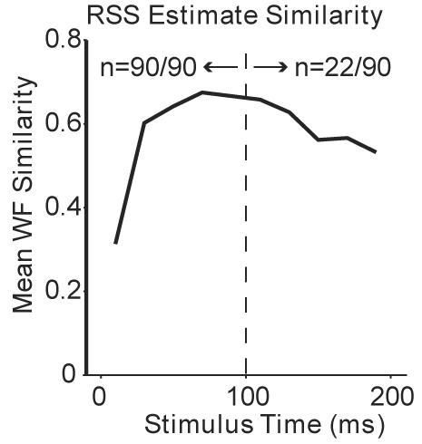
WF shape remains relatively constant throughout stimulus duration. Shown is mean WF similarity ≤ 100 ms (n = 90 neurons) and > 100 ms (n = 22 neurons).

Figure 3A shows the tuning of the neuron in Fig. 1 to tones and RSS, and Fig. 3B shows its OLS at different spectral contrast values. In the rate-level curves of Fig. 3C and the rate-contrast curves of Fig. 3D, this neuron can be seen to prefer high-contrast stimuli (22). Conversely, Fig. 3E shows a neuron with no response to tones at any frequency or sound level, although it did respond both to bandpass noise (BPN) of appropriate bandwidth and to RSS. When OLS at various contrasts (Fig. 3F) were delivered to the neuron, no sound level could be found at the highest contrast that elicited a vigorous response (Fig. 3G), yielding a nonmonotonic rate-contrast curve (Fig. 3H). Such a response pattern seems counterintuitive: High-contrast OLS contain more energy at the neuron's excitatory frequencies and less at its inhibitory frequencies than do low-contrast stimuli, yet the neuron prefers low to high contrast. This nonlinear behavior accounts for the neuron's preferential response to BPN (low local contrast) over tones (high contrast) without explicitly invoking arguments pertaining to neuronal bandwidth.

Fig. 3.

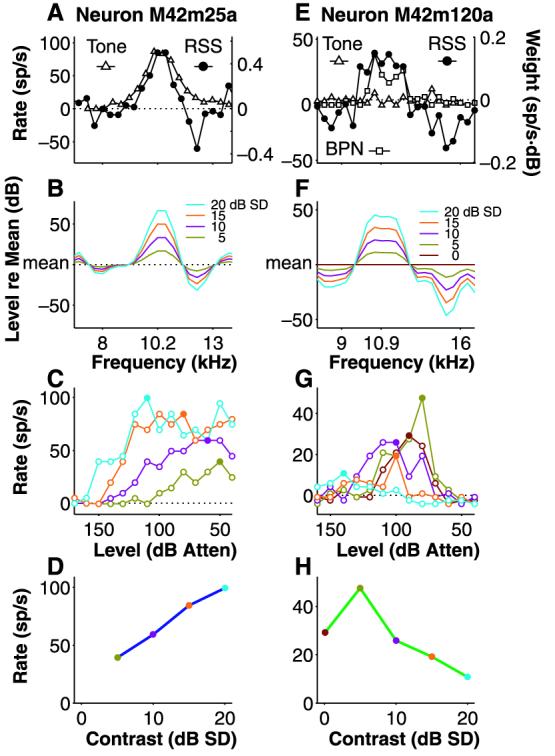
Two opposite responses to spectral contrast. (A) Tuning of the neuron in Fig. 1 to tones (△) as compared with RSS WF (●). (B) The WF was converted into OLS over several spectral contrast values (5 to 20 dB SD). Stimulus spectra were smoothed for illustration only. (C) Rate-level response curves for the four stimuli in (B). Lowest contrast elicited least response; highest contrast, greatest. Threshold shifts commonly occur as contrast is varied. (D) The peak rates from the rate-level curves in (C) (filled symbols) are plotted against stimulus contrast to produce a monotonic rate-contrast curve. (E) Tuning of another neuron to tones (△), 0.4-octave BPN (□), and RSS WF (●). (F) Smoothed spectra of OLS at contrast values of 0 to 20 dB SD. (G) Rate-level curves showing decreased responsiveness at the highest contrasts. (H) Rate-contrast curve revealing nonmono-tonic characteristics.

Rate-contrast curves are shown in Fig. 4A for high-contrast neurons and in Fig. 4B for low-contrast neurons. The population mean curve for each group can be seen in Fig. 4C, as well as histograms of contrast values at maximum response (rate-contrast peaks) in Fig. 4D. High-contrast neurons, on average, exhibit monotonic rate-contrast curves, whereas low-contrast neurons exhibit non-monotonic curves with lower rates overall. The mean rate-level curve for each group can be seen in Fig. 4E to be nonmonotonic for each type of neuron, although high-contrast neurons tend to have lower thresholds and spike at higher rates than do low-contrast neurons. Histograms reflecting the levels at the peaks of the rate-level curves (Fig. 4F) reveal no clear differences between the two types of neurons.

Fig. 4.

Population responses to spectral contrast. (A and B) Rate-contrast curves for 54 high- (blue) and 36 low- (green) contrast neurons. (C) Mean rate-contrast curves for high- and low-contrast neurons. Error bars show standard error of the mean (SEM). (D) Percentage of neurons whose rate-contrast peaks occurred at the given contrast values. (E) Mean ± SEM rate-level curves showing lower thresholds and higher rates for high- than for low-contrast neurons but similar shapes. (F) Percentage of neurons whose rate-level peaks occurred at the given sound levels. Magnitude of contrast preference (max absolute rate-contrast slope with sign preserved) are shown as a function of (G) CF and (H) orthogonal distance lateral to the lateral sulcus and (I) as a histogram.

A neuron is classified as high- or low-contrast by the sign of the greatest absolute slope of its rate-contrast curve. A plot of these slopes against CF (Fig. 4G) reveals that contrast preference has no apparent dependence on CF and consequently no apparent topographical distribution parallel to the lateral sulcus (23). On the other hand, a plot of the slopes against distance perpendicular to the lateral sulcus (Fig. 4H) reveals a potential tendency toward low-contrast neurons laterally (correlation coefficient of 0.20), which corresponds to the lateral belt area of AC. The distribution of contrast preferences appears to be unimodal and to peak around 0 (Fig. 4I), although as can be seen in Fig. 4, A and B, neurons with high maximum rates tend to have strong contrast preferences.

It has been suggested that the noise-preferring neurons of the lateral belt area exhibit bandwidth preferences (9), but such responses can be accounted for by contrast preference alone. At all CFs, AC neurons can be found that display either high- or low-contrast preference, implying that the full range of contrast preferences exists at all audible frequencies in marmosets (24). Because this range of CFs includes the frequencies of marmoset vocalization as well as head-related transfer function notches, contrast specificity may contribute to both sound recognition and localization. Neurons in the lateral belt area display a slightly greater propensity for low-contrast preference than do neurons in the A1 region, suggesting that contrast specificity could vary among cortical fields.

Contrast specificity appears to reflect a continuum of responses rather than two distinct classes; nevertheless, canonical responses of both types can be depicted (Fig. 5). High-contrast neurons respond poorly to or are inhibited by low-contrast stimuli and respond well to high-contrast stimuli. Low-contrast neurons respond poorly to or are inhibited by high-contrast stimuli, may respond moderately well to flat-spectrum stimuli (such as wideband noise), but respond best to stimuli of low contrast and appropriate spectra. High-contrast neurons may be modeled effectively as linear filters (25-28); low-contrast preference, on the other hand, reflects a nonlinear selectivity to wideband spectral profile. This finding holds strong implications for the neuronal coding of complex wideband stimuli such as animal vocalizations and human speech. Low-contrast neurons may be particularly useful for acoustic pattern recognition in background noise or when multiple competing signals are present (29).

Fig. 5.

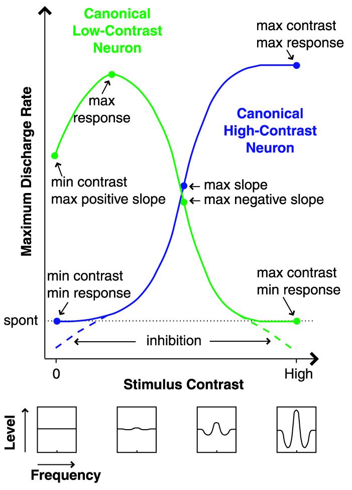
Canonical responses to spectral contrast. This coding scheme reflects complex multifrequency signal integration that cannot be predicted from frequency tuning alone. spont, spontaneous discharge rate.

References and Notes

- 1.Dan Y, Atick JJ, Reid RC. J. Neurosci. 1996;16:3351. doi: 10.1523/JNEUROSCI.16-10-03351.1996. [DOI] [PMC free article] [PubMed] [Google Scholar]
- 2.Olshausen BA, Field DJ. Nature. 1996;381:607. doi: 10.1038/381607a0. [DOI] [PubMed] [Google Scholar]
- 3.Schwartz O, Simoncelli EP. Nature Neurosci. 2001;4:819. doi: 10.1038/90526. [DOI] [PubMed] [Google Scholar]
- 4.Lewicki MS. Nature Neurosci. 2002;5:356. doi: 10.1038/nn831. [DOI] [PubMed] [Google Scholar]
- 5.Young ED. In: The Synaptic Organization of the Brain. Shepherd GM, editor. Oxford Univ. Press; New York: 1998. pp. 121–157. [Google Scholar]
- 6.Young ED. Proc. Natl. Acad. Sci. U.S.A. 1997;95:933. [Google Scholar]
- 7.Suga N. In: Auditory Function: Neurobiological Bases of Hearing. Edelman GM, Gall WE, Cowan WM, editors. Wiley & Sons; New York: 1988. pp. 679–720. [Google Scholar]
- 8.Suga N. In: The Cognitive Neurosciences. Gazzaniga MS, editor. Massachusetts Institute of Technology Press; Cambridge, MA: 1994. pp. 295–313. [Google Scholar]
- 9.Rauschecker JP, Tian B, Hauser M. Science. 1995;268:111. doi: 10.1126/science.7701330. [DOI] [PubMed] [Google Scholar]
- 10.Schreiner CE, Mendelson JR. J. Neurophysiol. 1990;64:1442. doi: 10.1152/jn.1990.64.5.1442. [DOI] [PubMed] [Google Scholar]
- 11.Schreiner CE, Mendelson JR, Sutter ML. J. Neurophysiol. 1992;68:1487. doi: 10.1152/jn.1992.68.5.1487. [DOI] [PubMed] [Google Scholar]
- 12.Peterson GE, Barney HL. J. Acoust. Soc. Am. 1952;24:175. [Google Scholar]
- 13.Wang X. Proc. Natl. Acad. Sci. U.S.A. 2003;97:11843. [Google Scholar]
- 14. RSS were similar to stimuli originally developed by E. D. Young for studying subcortical auditory neurons. Stimuli consisted of logarithmically spaced tones with amplitudes randomly distributed around a mean value. The tones were grouped into frequency bins such that all tones within a bin shared the same amplitude.
- 15. By collecting RSS sound-level deviations from the mean into a matrix Λ indexed by stimulus (rows) and frequency bin (columns), the driven rate (discharge rate–spontaneous rate) of a neuron can be approximated as a linear combination of frequency weights unique to the neuron: r = Λw + r0, where r is a vector of RSS-elicited driven rates, w is a vector of frequency weights, and r0 is a constant vector of rates in response to a wideband stimulus with all bins at the mean sound level. In practice, r is estimated directly from the stimulus presentations, and by designing Λ carefully (i.e., orthogonal, zero-mean columns), w can be estimated in a least-squares sense from west = α−1ΛTr, where α represents the single unique eigenvalue of the frequency autocorrelation matrix of Λ. This estimate represents a rate-weighted average wideband stimulus (the optimal linear stimulus) scaled by overall rate.
- 16.Ehret G, Merzenich MM. Science. 1985;227:1245. doi: 10.1126/science.3975613. [DOI] [PubMed] [Google Scholar]
- 17.Ehret G, Merzenich MM. Brain Res. 1988;472:139. doi: 10.1016/0165-0173(88)90018-5. [DOI] [PubMed] [Google Scholar]
- 18.Calhoun BM, Miller RL, Wong JC, Young ED. In: Psychophysical and Physiological Advances in Hearing. Palmer AR, Rees A, Summerfield AQ, Meddis R, editors. Whurr Publishers; London: 1998. pp. 170–177. [Google Scholar]
- 19.Yu JJ, Young ED. Proc. Natl. Acad. Sci. U.S.A. 2000;97:11780. doi: 10.1073/pnas.97.22.11780. [DOI] [PMC free article] [PubMed] [Google Scholar]
- 20. Extracellular recording methods have been described previously (29). Neurons were isolated from all cortical layers and were sampled on the superior temporal gyrus from the lateral sulcus medially to non-auditory areas laterally. This region comprises A1 and the lateral belt. OLS have spectral profiles matching a neuron's WF.
- 21. WF similarity curves compared WFs computed from spikes in each 20-ms interval of stimulus duration with a WF computed from spikes throughout the stimulus interval. Similarity measures between each pair of WF vectors were normalized inner products, which could take on values in the range [−1, 1] (perfect match was 1, chance value was 0). All 90 neurons were studied with stimuli at least 100 ms in duration; 22 neurons were studied with longer stimuli.
- 22. Rate-level curves were constructed by varying the mean level of the OLS at a fixed contrast and measuring the corresponding rate. Rate-contrast curves were constructed by taking the peak of the rate-level curve at each contrast value.
- 23.Aitkin LM, Merzenich MM, Irvine DR, Clarey JC, Nelson JE. J. Comp. Neurol. 1986;252:175. doi: 10.1002/cne.902520204. [DOI] [PubMed] [Google Scholar]
- 24.Seiden HR. Princeton University; Princeton, NJ: 1957. thesis. [Google Scholar]
- 25.Schreiner CE, Calhoun BM. Aud. Neurosci. 1994;1:39. [Google Scholar]
- 26.Kowalski N, Depireux DA, Shamma SA. J. Neurophysiol. 1996;76:3524. doi: 10.1152/jn.1996.76.5.3524. [DOI] [PubMed] [Google Scholar]
- 27.deCharms RC, Blake DT, Merzenich MM. Science. 1998;280:1439. doi: 10.1126/science.280.5368.1439. [DOI] [PubMed] [Google Scholar]
- 28.Schnupp JW, Mrsic-Flogel TD, King AJ. Nature. 2001;414:200. doi: 10.1038/35102568. [DOI] [PubMed] [Google Scholar]
- 29.Barbour DL, Wang X. J. Neurophysiol. 2002;88:2684. doi: 10.1152/jn.00253.2002. [DOI] [PubMed] [Google Scholar]
- 30. We thank E. D. Young for generously sharing the theory behind RSS, E. Bartlett for comments on a previous version of this manuscript, and A. Pistorio for assistance in animal training and graphic design. Supported by NIH grant DC–03180 and a Presidential Early Career Award for Scientists and Engineers (X.W.).