Quantifying Robustness and Dissipation Cost of Yeast Cell Cycle Network: The Funneled Energy Landscape Perspectives

Abstract

We study the origin of robustness of yeast cell cycle cellular network through uncovering its underlying energy landscape. This is realized from the information of the steady-state probabilities by solving a discrete set of kinetic master equations for the network. We discovered that the potential landscape of yeast cell cycle network is funneled toward the global minimum, G1 state. The ratio of the energy gap between G1 and average versus roughness of the landscape termed as robustness ratio (RR) becomes a quantitative measure of the robustness and stability for the network. The funneled landscape is quite robust against random perturbations from the inherent wiring or connections of the network. There exists a global phase transition between the more sensitive response or less self-degradation phase leading to underlying funneled global landscape with large RR, and insensitive response or more self-degradation phase leading to shallower underlying landscape of the network with small RR. Furthermore, we show that the more robust landscape also leads to less dissipation cost of the network. Least dissipation and robust landscape might be a realization of Darwinian principle of natural selection at cellular network level. It may provide an optimal criterion for network wiring connections and design.

INTRODUCTION

Energy landscape and cellular network

To understand the biological function and robustness of the cellular network, it is crucial to uncover the underlying global principle (1–3). The natures of the cellular network have been explored by many experimental techniques (4). It is found that the cellular networks are in general quite robust against genetic and environmental perturbations. There have been an increasing number of studies on the global topological structures of the networks recently (5–8). However, there are so far very few studies of why the network should be robust and perform the biological function from the physical point of view (9–22).

Theoretical models of the cellular networks have often been formulated with a set of deterministic chemical rate equations. These dynamical descriptions are inherently local. To probe the global properties, one often has to change the parameters. The parameter space is huge. The global robustness therefore is hard to see from this approach.

Here we will explore the nature of the network from another angle: formulate the problem in terms of the potential function or potential landscape. If the potential landscape of the cellular network is known, the global properties can be explored (13,15–18,20–24). This is in analogy with the fact that the global thermodynamic properties can be explored when knowing the inherent interaction potentials in the system. In the cell, statistical fluctuations coming from the finite number of molecules (typically on the order of 1–1000) provide the source of intrinsic internal noise and the fluctuations from highly dynamical and inhomogeneous environments of the interior of the cell provide the source of the external noise for the networks (25–30). Both the internal and external noise play important roles in determining the properties of the network.

In general, one should study the chemical reaction network equations in the noisy conditions to model the cellular environments more realistically. In other words, instead of following the deterministic evolution of the concentrations of proteins in the network by the normal chemical rate equations, one should describe the dynamics of protein concentrations probabilistically. We can realize this through the kinetic master equations. We can study the steady-state probability distributions of these chemical concentrations under noisy environments. The generalized potential function for steady state of the network is closely associated with the steady-state probability (13,15–18,20–22,31). Once the network problem is formulated in terms of the generalized potential function or the potential landscape, the issue of the global stability or robustness is much easier to address. In fact, an explicit illustration of energy landscape and robustness for MAP Kinase signal transduction network has been given recently (20–22).

It is the purpose of this article to study the global robustness problem directly from the properties of the potential landscape for the budding yeast cell cycle network. Furthermore, cellular network is an open nonequilibrium system due to the interactions with the environments. There is a dissipation cost associated with the network. It will also be interesting to see for our model system how the dissipation cost is related to the features of the landscape reflecting the stability and robustness.

Budding yeast cell cycle

To explore the nature of the underlying potential landscape of the cellular network, we will study the budding yeast cell cycle network. One of the most important functions of the cell is the reproduction and growth. It is therefore crucial to understand the cell cycle and its underlying process. The cell cycles during the development are usually divided in several phases: G1 phase, in which cell starts to grow under appropriate conditions; S phase, in which DNA synthesis and chromosome replication occurs; G2 phase, where the cell is in the stage of preparation for mitosis; and M phase, in which chromosome separation and cell division occurs. After passing through the M phase, the cell enters back to G1 phase and thus completes a cell cycle. In most of the eukaryotic cells, the elaborate control mechanisms over DNA synthesis and mitosis make sure the crucial events in the cell cycle are carried out properly and precisely. Physiologically, there are usually several check points (where cells are in the quiescent phase waiting for the signal and suitable conditions for further progress in the cell cycle) for controlling and coordination: G1 before the new round of division; G2 before the mitotic process begins; and M before segregation.

Recently, many of the underlying controlling mechanisms are revealed by the genetic techniques such as mutations or gene knockouts. It is found that control has been centered around cyclin-dependent protein kinases (CDKs), which trigger the major events of the eukaryotic cell cycle. For example, the activation of cyclin/CDK dimer drives the cells at both G1 and G2 checkpoints for further progress. During other phases, check points CDK/cyclin are activated. Although molecular interactions regulating the CDK activities are known, the mechanisms of the checkpoint controls are still uncertain (9–12).

The cell cycle process has been studied in details in the budding yeast Saccharomyces cerevisiae (4,9–12,14). There are many genes involved in controlling the cell cycle processes. However, the number of the crucial regulators is much less. A network-wiring diagram based on the crucial regulators can be constructed (9–12,14) as shown in Fig. 1.

FIGURE 1.

The yeast cell cycle network scheme: wiring diagram, the arrow sign (→) represents positive activating regulations (1); the inhibition sign (⊣) represents negative suppressing regulations (−1); and the loop sign (•••|) represents self-degradation.

Under the rich nutrient conditions, when the cell size grows large enough, a cyclin Cln3 will be turned on. Thus, the cell-cycle sequence starts when the cell commits to division through the activation of Cln3 (the START). The Cln3/Cdc28 will be activated. This in turn activates through phosphorylation a pair of transcription factor groups, SBF and MBF, which activate the genes of the cyclins Cln1 and Cln2 and Clb5 and Clb6, respectively. The subsequent activity of Clb5 drives the cell into the S phase where DNA replication begins. The entry into the M phase for segregation is controlled by the activation of Clb2 through the transcription factor MCM1/SFF activation. The exit of the M phase is controlled by the inhibition and degradation of Clb2 through the Sic1, Cdh1, and Cdc20. Clb2 phosphorylates Swi5 to prevent its entry into the nucleus. After the M phase, the cell comes back to the stationary G1 phase, waiting for the signal for another round of division. Thus, the cell-cycle process starts with the excitation from the stationary G1 state by the cell-size signal and evolves back to the stationary G1 state through a well-defined sequence of states.

Mathematical models of the cell cycle controls have been formulated with a set of ordinary first-order (in time) differential equations mimicking the underlined biochemical processes (9–12,14). The models have been applied to the budding yeast cycle and explained many qualitative physiological behaviors. The checkpoints can be viewed as the steady states or stationary fixed points. Since the intracellular and intercellular signals are transduced into the changes in the regulatory networks, the cell cycle becomes the dynamics in and out of the fixed points. Although detailed simulations give some insights toward the issues, due to the limitation of the parameter space search, it is difficult to perceive the global or universal properties of the cycle networks (for example, for different species). It is the purpose of the current study to address this issue.

We will study the global stability by exploring the underlying potential landscape for yeast cell cycle network.

MATERIALS AND METHODS

The average dynamics of the network can be usually described by a set of chemical rate equations for concentrations where both the concentrations and the links among them through binding rates with typically quite different timescales are treated in a continuous fashion. In the cycle, most of the biological functions seem to be from the on- and off-properties of the network components. Further more, the global properties of the network might depend less sensitively on the details of the model. Therefore, a simplified representation (14) can be proposed with each node i having only two states, S_i = 1 and S_i = 0, representing the active and the inactive state of the protein, or high concentration and low concentration of proteins, respectively. As illustrated in Fig. 1, we have 11 protein nodes in the network wiring diagram; altogether, we have 2¹¹ states, each state represented by S, with a distinct combination of the on and off of the 11 protein nodes of Cln3, MBF, SBF, Cln1-2, Cdh1, Swi5, Cdc20, Clb5-6, Sic1, Clb1-2, and Mcm1 represented by {S₁, S₂, S₃, …S₁₁} = S. The arrows (→) represent positive regulations or activations (1). Inhibition sign (—|) represent negative regulations or repressions (−1). The loop (—|) represents self-degradations to the nodes which are not regulated by others. We can then define some rules to follow the subsequent dynamics of the network. Therefore, the evolution of the network is deterministic.

As mentioned, in the cell the average dynamics of the cellular network might not give a good description of the system. This is due to the intrinsic fluctuations from the limited number of the proteins in the cell and extrinsic fluctuations from the environments in the interior of the cell. It is then more appropriate to approach the network dynamics based on statistical description. In other words, we should replace the deterministic or average description of the dynamics of states in cellular network to a probabilistic description of the evolution of the cellular network dynamics. Therefore, instead of following the on- and off-state switching in the network, we follow the probability of on and off for each state in the network.

To follow the evolution of the states in the cellular network, we need to first figure out the transition probability from one state S₁ at present time to another state S₂ at the next moment. This is difficult to solve and in general almost impossible. We therefore will make some simplifications so that we can handle the case without the loss of the generality by assuming that the transition probability T from one state to another can be split into the product of the transition probability for each individual flip (or no flip) of the on- or off-state from this moment to the next moment. The transition probability from one state at current state to another at next moment will be assumed not to depend on the earlier times (no memory). This leads to the Markovian process (32–34). The transition matrix T can thus be written as

(1)

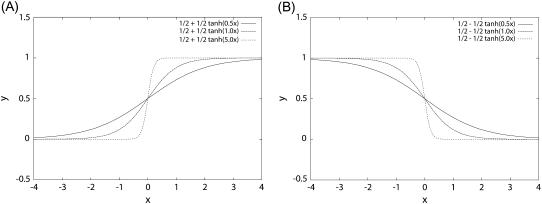
where t is the current time and t′ is the next moment. So the whole transition probability from current state to the next is split into the product of the transition probability of each individual flip (or no flip) of the node i. For each individual flip, the transition probability for a particular node can be modeled as a nonlinear switching function as shown in Fig. 2, A and B, from the input through the interactions to the output, which is often used in neural science (35):

(2)

When the input is positive (activation), the transition probability to the on-state is higher (close to 1). When the input is negative (repression), the transition probability to the on-state is lower (close to zero). Furthermore

(3)

when there is no input of activation or repression (), and c is a small number mimicking the effect of self-degradation. Here a_ij is the arrow or link representing the activating (+1) or suppressing (−1) interactions between i^th and j^th protein node in the network, which is explicitly shown in the wiring diagram of Fig. 1. The value μ is a parameter controlling the width of the switching function from the input to the output. The physical meaning is clear. If the inputs through the interactions among proteins to a specific protein node in the network are large enough, then the state will flip, otherwise the state will stay without the flip. The positive (negative) sign in the T expression gives probability of flipping from 0(1) to 1(0) state as well as from 1(0) to 1(0). If μ is small (large), the transition width is large (small), the transition is smooth (sharp or sensitive) from the original state to the output state. Therefore, we have an analytical expression of the transition probability.

FIGURE 2.

Nonlinear response function versus inputs: Fig. 2 A is for y = 1/2 + 1/2tanh(μx) when μ = 0.5, 1, 5 and Fig. 2 B is for y = 1/2 − 1/2tanh(μx) when μ = 0.5, 1, 5.

With the transition probability among different states specified, finally we can write down the master equation for each of the 2¹¹ states as

(4)

where T_ij (T_ji) represents the transition probability from state i(j) to state j(i) specified in details above. Here i and j are from 1 to 2¹¹ = 2048 states and

We solved the 2¹¹ = 2048 master equations numerically of the yeast cell cycle (by using iterative method) to follow the evolution of the probability distribution of each state, with the initial condition of equal small probability of all the cell states (P_i = 1/2048). Both the time-dependent evolution and the steady-state probability distribution for each state are obtained.

Let us focus on the steady-state probability distribution. For each state, there is a probability associated with it. One can write the probability distribution for a particular state as P_i = exp[ − U_i] () or U_i = − lnP_i. One can immediately see that U_i acquires the meaning of generalized potential energy (from Boltzmann distribution). This is the key point: although there is no potential energy function directly from the normal deterministic averaged chemical reaction rate equations for the network, a generalized potential energy function does exist and can be constructed from the probabilistic description of the network instead of the deterministic averaged one. This generalized potential energy function is inversely related to the steady-state probability. When the probability is large, the potential energy is lower and when probability is small, the potential energy is higher. The dynamics of the cell cycle thus can be visualized as passing through mountains and ridges of the energy landscape in state space of the cell cycle network to the final destiny. The advantage of introducing the concept of energy is that once we have the potential landscape, we can discuss the global stability of the protein cellular networks. Otherwise, it is almost impossible to address the global issues without going through the parameter space locally, which is often cosmologically big.

The network is an open system in nonequilibrium state. Even at steady state, the system is not necessarily in equilibrium. This is clear from the fact that although we can obtain the steady-state probability and can define an equilibrium-like quantity such as steady-state probability, the flux is not necessarily equal to zero (F_{ijsteady-state} = − T_ijP_{isteady-state} + T_jiP_{jsteady-state}). This is different from the equilibrium situation where the local flux is equal to zero (detailed balance condition). The flux defines a generalized force for the nonequilibrium steady state along with the associated generalized chemical potential (37). The nonequilibrium steady state dissipates energy. In the steady state, the heat loss rate is equivalent to entropy production rate, where entropy S₀ is defined as and entropy production rate (per unit time) S is given by

(5)

Entropy production rate is a characterization of the global properties of the network. We can study how the entropy production rate or dissipation cost of the network changes with the global structure and underlying landscape of the network, as well as how it varies with the changes of internal and external perturbations. We can explore the global natures of the network such as stability, robustness, and dissipation cost and their interrelationships.

In each of the simulations, we study the robustness of the network by exploring different values of switching and self-degradation parameters μ and c, as well as the mutations of the links or interactions in the network.

RESULTS AND DISCUSSION

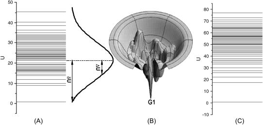
Since the potential energy is a multidimensional function in protein states, it is difficult to visualize U. Therefore, we directly look at the energy spectrum (Fig. 3) and explore the nature of the underlying potential landscape U.

FIGURE 3.

The global structures and properties of the underlying potential landscape of the yeast cell cycle network. (A) The spectrum and the histogram or the distribution of the potential energy U. (B) An illustration of the funneled landscape of the yeast cell cycle network. The global minimum of the energy is at G1 state. (C) The spectrum of the potential energy U for a random network.

Fig. 3 A shows the spectrum as well as the histogram of U. We can see that the distribution is approximately Gaussian. The lowest potential U is the global minimum of the potential landscape. It is important to notice this global minimum of U is found to be the same state as the steady state or fixed point (the stationary G1 state = (0;0;0;0;1;0;0;0;1;0;0)) of the deterministic averaged chemical reaction network equations for the yeast cell cycle. It is clear that the global minimum of the potential is significantly separated from the average of the potential spectrum or distribution.

To quantify this, we define the robustness ratio RR for the network as the ratio of the gap δU, the difference between this global minimum of G1 state U_{global-minimum} and the average of U, 〈U〉 versus the spread or the half-width of the distribution of U, ΔU, as shown in Fig. 3 A. The value δU is a measure of the bias or the slope toward the global minimum (G1 state) of the potential landscape. ΔU is a measure of the averaged roughness or the local trapping of the potential landscape. When RR is significantly >1, the gap is significantly larger than the roughness or local trapping of the underlying landscape, then the global minimum (G1 state) is well separated and distinct from the average of the network potential spectrum. Since P_i = exp{−U(x)}, the weight or population of the global minimum (G1 state) will be dominated by the one with large RR. The populations of the other possible states are much less significant. This leads to the global stability or robustness discriminating against others. The RR value for the yeast cell cycle network is RR = 3 (for μ = 5 and c = 0.001) as shown in Fig. 3 A, significantly larger than 1. This shows a funnel picture of energy going downhill toward G1 state in the evolution of network states, as illustrated in Fig. 3 B. Therefore, RR gives a quantitative measure of the property of the underlying landscape spectrum.

We found the typical values for random networks are close to 2 (RR cannot be <1). A typical random network with RR 2 is illustrated in Fig. 3 C for a random network. The ground state, however, is not necessarily the G1 state any more. The probability of G1 is smaller for the random network compared with the biological one and therefore less stable. Comparing the two potential energy spectra, we found the spread or the dispersion ΔU for the random network in Fig. 3 C is larger than the biological network in Fig. 3 A. Thus, the robustness ratio RR = δU/ΔU for random network is smaller than the biological one. Only the cellular network landscape with a large value of RR will be able to form a stable global minimum G1 state, be robust, perform biological functions, and survive the natural evolution.

We identified the preferential global pathway toward the global minimum G1 by following the most probable trajectory in each step of the kinetic moves from the kinetic master equations toward G1. The protein can be either 1 or 0 representing active or inactive. The 11 proteins are arranged in a vector form to represent the state of the system as (Cln3; MBF; SBF; Cln1,2; Cdh1; Swi5; Cdc20; Clb5, 6; Sic1; Clb1,2; Mcm1).

The most probable global path follows the states 1→13 sequentially toward G1 from the start signal, where:

• The start signal is in state sequence 1, as given by (1;0;0;0;1;0;0;0;1;0;0).

• Three excited G1 states are in sequences 2–4, given, respectively, by (0;1;1;0;1;0;0;0;1;0;0), (0;1;1;1;1;0;0;0;1;0;0), and (0;1;1;1;0;0;0;0;0;0;0).

• The S phase is in a state with sequence 5 given by (0;1;1;1;0;0;0;1;0;0;0).

• The G2 phase is in a state with sequence 6 given by (0;1;1;1;0;0;0;1;0;1;1).

• The M phase is in states with sequences 7–11, given, respectively, by (0;0;0;1;0;0;1;1;0;1;1), (0;0;0;0;0;1;1;0;0;1;1), (0;0;0;0;0;1;1;0;1;1;1), (0;0;0;0;0;1;1;0;1;0;1), and (0;0;0;0;1;1;1;0;1;0;0).

• The other excited G1 state is in sequence 12, given by (0;0;0;0;1;1;0;0;1;0;0).

• Finally, stationary G1 phase is in state sequence 13, given by (0;0;0;0;1;0;0;0;1;0;0).

The most probable path turns out to be the biological path going through G1→S→G2→M→G1.

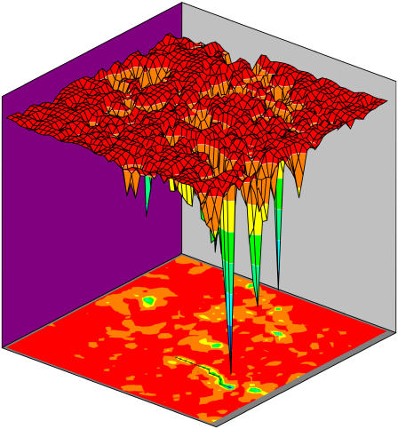
We arranged the state space into the two-dimensional grids with the constraints of minimal overlapping or crossings of the state connectivity for the purpose of clear visualization. Each point on the two-dimensional grid represents a state (one of 2048 states). The energy landscape on the two-dimensional grids is shown in Fig. 4. The lowest energy state corresponds to the stationary G1 state. The global biological path is represented by the narrow green band on the projected two-dimensional-state space plane with small arrows connecting each relevant state. It is sequentially from state 1–13 as mentioned in the above text (sequences 1→13). As we can see, the global biological path lies in the low energy valley of the landscape toward G1. In addition, we can also see some other off-pathway traps (states with low energies).

FIGURE 4.

The potential energy landscape of the yeast cell cycle network and biological path to stationary G1: The lowest energy state corresponds to stationary G1 state. The green band with arrows corresponds to the biological path (sequentially from state 1 to 13 described in the text).

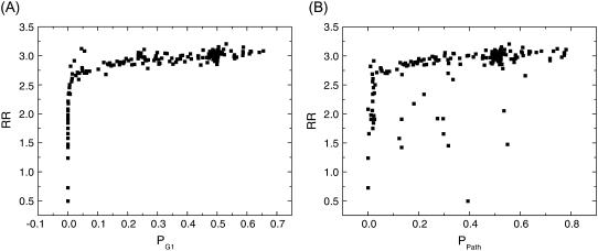
Fig. 5 A shows robustness ratio, RR of the cell cycle network versus the steady-state probability of the G1 (with μ = 5 and c = 0.001) against various perturbations. These perturbations are through deleting an interaction arrow, adding an activating or repressing arrow between the nodes that are not yet connected in the network wiring diagram in Fig. 1, or switching an activating arrow to a repressing arrow or vice versa, and deleting an individual node. There is a monotonic relationship between the G1 probability and robustness ratio RR. When RR is larger (smaller), the landscape is more (less) robust, the network is more (less) stable with G1 state dominating (less significant). Therefore, RR is indeed a robustness measure for the network.

FIGURE 5.

Robustness against mutation perturbations. (A) Robustness ratio versus steady-state probability of G1, P_G1 for different mutations of the links. (B) Robustness ratio RR versus steady-state probability of biological path, P_path for different mutations of the links.

Fig. 5 B shows the robustness ratio RR versus steady-state probability of the global biological path with important biological states including G1 (14). We see again that network with large RR characterizing the funneled landscape leads to higher steady-state probability and therefore more stable biological path. Random networks typically have smaller RR and smaller probability of G1 compared with the biological one. They are less stable. The biological functioning network is quite different from the random ones in terms of the underlying energy landscape and stability.

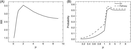
Fig. 6 A shows the robustness ratio of the underlying energy landscape versus different switching parameters μ (c = 0.001). We see that when μ is large (small) indicating a sharp (smooth) transition or response from input to output for a single flip of the protein states, the robustness ratio increases with μ increases. This means a sharper transition or response from input to output gives more a robust network compared with the smoother transition or response. The value μ can also be seen as a measure or characterization of the strengths of the noise from the intrinsic or extrinsic statistical fluctuations in the cellular environments (36). The μ could then be related to the inverse of the temperature (temperature here is a measure of the strength of the noise level). The energy U we defined in this article is in units of μ. Therefore, U is a dimensionless quantity. When μ is not changing, the two definitions of U (U = −μlogP and U = −logP) are only different by a constant. The RR is not influenced by the above two definitions of U since it involves the ratio of the U-values.

FIGURE 6.

Robustness against the sharpness of the response or the inverse noise level. (A) Robustness ratio versus sharpness of the response or inverse of noise level μ. (B) Steady-state probability of stationary G1, P_G1 and biological path, P_path versus μ.

When μ is large, the transition is sharp. This corresponds to all-or-none deterministic behavior for the response or transition (0 or 1). This is the situation when the underlying statistical fluctuations are small. When μ is small, the response or the transition is no longer all-or-none (1 or 0) but a smooth function in between 0 and 1. This is due to the fact the statistical fluctuations lead to the states more distributed and with less sharp response. Therefore, the associated probability of distributed states has more chances being between 0 and 1. In other words, less (more) statistical fluctuations or shaper response with larger μ (less sensitive response with smaller μ) leads to more (less) robust network characterized by large (small) RR. Then, there exist two phases for the network: a robust phase with RR is significantly larger than 2, where the network is stable and the underlying energy landscape is funneled toward G1; and a fragile phase with RR drops to ≤2, where the network is less stable and the underlying energy landscape is shallower toward G1.

Fig. 6 B shows probability of stationary G1 state as well as the probability of the global path toward G1 versus μ. We can see a global transition phase transition at μ ∼ 1, below which P_G1 and P_path significantly drops. From Fig. 6, A and B, we see when P_G1 and P_path is small, RR is also small, implying the system is less stable. Therefore, the network loses the stability below μ ∼ 1. Significantly above μ ∼ 1, the network becomes stable. We can interpret this as the phase transition from the weak noise limit where the underlying landscape and the associated global path are not influenced much by the noise level to the limit where underlying landscape and associated global path are disturbed significantly or disrupted by the strong noise. We can also interpret this as the transition from hypersensitive response leading to the robustness of the landscape and the associated global path, to the inert or insensitive response leading to the fragile landscape and associated global path to G1. We can see a sharper response or more sensitivity of the individual protein nodes to the rest of the protein network through interactions usually leads to more robustness of the network with stable G1 and biological path.

The low μ corresponds to strong noise limit or insensitive response for the node to the input. The landscape has low RR and is less stable or robust. The landscape is more flat and less biased toward G1. When μ increases, the noise level decreases, the response to the input is more sensitive for each node. This results in a more funneled topography toward G1 and a more robust landscape. The maximal funnel is found at ∼μ = 2. There is a sharp change of the shape of the landscape near μ = 2 from the μ < 2 side. When μ > 2, the RR value is slightly lower and quickly approaches to a constant as μ becomes larger, corresponding to smaller noise and a more sensitive response from a node to the input. The landscape becomes stabilized with a definite robustness ratio and probability of P_G1. The peak value of the RR, P_G1 as well as P_path implies that traps might exist in the landscape (deep energy states other than G1 and not on biological path). Large noise will destroy landscape, which leads to low RR, P_G1 as well as P_path. Zero noise leads to relatively stable network with relatively large RR, P_G1 as well as P_path. In the presence of traps, adding a small amount of noise helps the system to reach the global minimum without getting caught or trapped in the intermediate off-pathway trapping states. This increases the probability and enhances the stability of G1 and biological path. Therefore, the presence of the peak of RR, P_G1 as well as P_path is an indication of the existence of traps in the landscape. We found six major off-pathway traps responsible for the peak in RR, P_G1 as well as P_path (some are shown in Fig. 4).

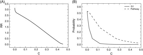
Fig. 7 A shows the robustness ratio of the underlying energy landscape versus different self-degradation parameters c (at μ = 5). We see that when c is large (small) indicating a large (small) self-degradation, the robustness ratio increases with c decreases. This means less degradation gives a more robust network. Fig. 7 B shows the probability of stationary G1 as well as biological path versus different self-degradation parameters c (at μ = 5). We see that when c is large (small) indicating a large (small) self-degradation, the probability of stationary G1 phase and biological path increases with decrease of c parameters. This means less degradation gives a more probable and stable stationary G1 phase and biological path, and therefore a more robust network.

FIGURE 7.

Robustness against self-degradation. (A) Robustness ratio RR versus degree of self-degradation, c. (B) Steady-state probability of stationary P_G1 and biological path P_path versus c.

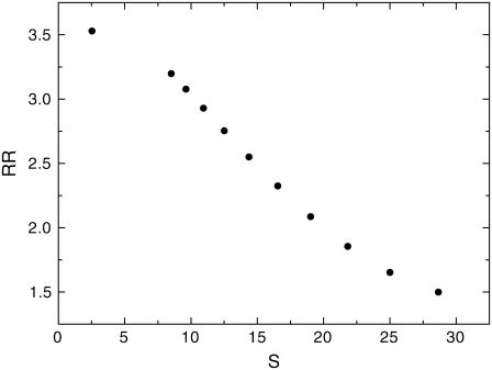
In Fig. 8, we plotted the entropy production (per unit time) or the dissipation cost of the network, S, versus RR for different μ. We can see the entropy production rate decreases as RR increases. This implies the more robust the network is, the less entropy production or heat loss the network has. This can be very important for the network design. The nature might evolve such that the network is robust against internal (intrinsic) and environmental perturbations, and perform specific biological functions with minimum dissipation cost. The fact that robustness is linked with the entropy production rate may reflect that fewer fluctuations and perturbations lead to more robust and stable networks as well as more energy saved, and therefore lower costs in mean time. This might provide us a design principle of optimizing the connections of the network with minimum dissipation cost for the network. In this study, it is also the equivalent of optimizing the robustness or stability of the network.

FIGURE 8.

Dissipation cost versus robustness of the network: entropy production rate S versus robustness ratio RR.

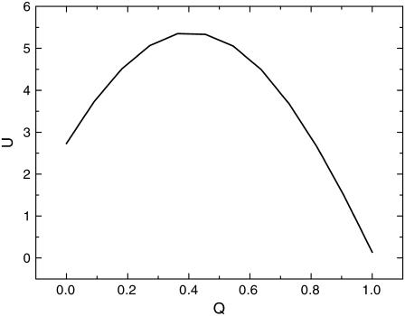
In Fig. 9, we define an order parameter Q for this model, based on how many nodes there are in the same state relative to the stationary G1 phase, normalized to 1. So Q = 1 when the network is in stationary G1 phase, and Q = 0 when the network is in a state, which is completely uncorrelated with the stationary G1 phase. We plotted the projection of energy U to the order parameter Q. We can see that there are two minimum or two basins of attraction. One is at Q = 1. It is the global minimum corresponding to the global stationary G1 phase. The other is near Q = 0, corresponding to the G2 phase. The existence of different basins of attraction is reasonable in the cell cycle network with several checkpoints. One of the major checkpoints in the experiments turns out to be G2. So checkpoints could be seen as on pathway “trapping.” The robustness network will be able to pull out itself from the on pathway “trapping” to precede the normal cell cycle function to G1.

FIGURE 9.

One-dimensional projection of the energy landscape: potential U versus fraction of protein nodes consistent with the stationary G1 phase, Q.

CONCLUSIONS

The energy landscape is a statistical-based approach, which is good in two ways: It is an approach capturing the global properties; and, on the other hand, the statistical approach can be very useful and informative when the data are rapidly accumulating. In this picture, there are many possible energy states of the network corresponding to different patterns of combinations of activation and inhibition of the protein states. Each checkpoint can be viewed as basins of attraction of globally low energy states. The G1 phase states have the lowest global energy since they are at the end of the cycle. We believe it might be possible to describe the cell cycle as the dynamic motion in the energy-landscape-state space from one basin to another. This kinetic search cannot be entirely random but directed since the random search takes cosmological time. The direction or gradient of the landscape is provided from the bias in terms of the energy gap toward the G1 phase. Therefore, the landscape picture is one is which there is a funnel toward the G1 state (the bottom of the funnel, which we can call native state). At the end of G1 phase, the network is pumped upon receiving the new start signal through further nutrition supply, without which the system will stay at G1 and network cannot continue the cycling process) to high energy excited states at the top of the funnel (cycling). Then the cell cycle follows as it cascades through the configurational state space (or energy landscape) in a directed way passing several checkpoints (basins of attraction) and finally reach the bottom of the funnel-G1 phase before being pumped again for another cycle (Fig. 4).

We can see from the above discussions that maximizing the ratio of the potential gap (or the slope) versus the roughness of the underlying potential landscape is the criterion for the global stability or robustness of the network. Only the cellular network landscape satisfying this criterion will be able to form a thermodynamically stable global steady state, be robust (Fig. 5–7), perform the biological functions with minimal dissipation cost (Fig. 8), and survive the natural evolution. Similar to a protein folding and binding problem (38,39), a funneled potential landscape of cellular network emerges. The landscape biases toward the global minimum G1 state and dominates the fluctuations or wiggles in the configurational space. From this picture, at the initial stage of the yeast cell cycle network process, there could be multiple parallel paths leading toward the global minimum G1 state. As the kinetic process progresses, the discrete paths might emerge and give dominant contributions (biological path) when the roughness of the underlying landscape becomes significant (Fig. 4).

The cellular network with too-rough an underlying potential landscape can neither guarantee the global robustness nor perform specific biological functions. They are more likely to phase out from evolution. The funneled landscape therefore is a realization of Darwinian principle of natural selection at the cellular network level. As we see, the funneled landscape provides an optimal criterion to select the suitable parameter subspace of cellular networks, guarantees the robustness, and performs specific biological functions with less dissipation cost. This will lead to an optimal way for the network connections and is potentially useful for the network design.

It is worth pointing out that the approach described here is general and can be applied to many cellular networks such as a signaling transduction network (2) and a metabolic network (40), where there might be only one funnel dominating, and a gene regulatory network where multiple (yet finite number of) funnels or basins of attraction emerge (13,16,22).

References

- 1.Davidson, E. H., J. P. Rast, P. Oliveri, A. Ransick, C. Calestani, C.-H. Yuh, T. Minokawa, G. Amore, V. Hinman, C. Arenas-Mena, O. Otim, C. T. Brown, C. Livi, P. Y. Lee, R. Revilla, A. G. Rust, Z. J. Pan, M. J. Schilstra, P. J. C. Clarke, M. I. Arnone, L. Rowen, R. A. Cameron, D. R. McClay, L. Hood, and H. Bolouri. 2002. A genomic regulatory network for development. Science. 295:1669–1673. [DOI] [PubMed] [Google Scholar]
- 2.Huang, C. Y., and J. E. Ferrell, Jr. 1996. Ultrasensitivity in the mitogen-activated protein kinase cascade. Proc. Natl. Acad. Sci. USA. 93:10078–10082. [DOI] [PMC free article] [PubMed] [Google Scholar]
- 3.Kholodenko, B. N. 2000. Negative feedback and ultrasensitivity can bring about oscillations in the mitogen-activated protein kinase cascades. Eur. J. Biochem. 267:1583–1593. [DOI] [PubMed] [Google Scholar]
- 4.Ideker, T., V. Thorsson, J. A. Ranish, R. Christmas, J. Buhler, J. K. Eng, R. Bumgarner, D. R. Goodlett, R. Aebersold, and L. Hood. 2001. Integrated genomic and proteomic analyses of a systematically perturbed metabolic network. Science. 292:929–933. [DOI] [PubMed] [Google Scholar]
- 5.Jeong, H., B. Tombor, R. Albert, Z. N. Oltvai, and A. L. Barabasi. 2000. The large-scale organization of metabolic networks. Nature. 407:651–654. [DOI] [PubMed] [Google Scholar]
- 6.Barabasi, A. L., and E. Bonabeau. 2003. Scale-free networks. Sci. Am. 288:60–69. [DOI] [PubMed] [Google Scholar]
- 7.Maslov, S., and K. Sneppen. 2002. Specificity and stability in topology of protein networks. Science. 296:910–913. [DOI] [PubMed] [Google Scholar]
- 8.Milo, R., S. Shen-Orr, S. Itzkovitz, N. Kashtan, D. Chklovskii, and U. Alon. 2002. Network motifs: simple building blocks of complex networks. Science. 298:824–827. [DOI] [PubMed] [Google Scholar]
- 9.Tyson, J. J., K. Chen, and B. Novak. 2001. Network dynamics and cell physiology. Nat. Rev. Mol. Cell Biol. 2:908–916. [DOI] [PubMed] [Google Scholar]
- 10.Novak, B., and J. J. Tyson. 1997. Modeling the control of DNA replication in fission yeast. Proc. Natl. Acad. Sci. USA. 94:9147–9152. [DOI] [PMC free article] [PubMed] [Google Scholar]
- 11.Tyson, J. J. 1991. Modeling the cell division cycle: cdc2 and cyclin interactions. Proc. Natl. Acad. Sci. USA. 88:7328–7332. [DOI] [PMC free article] [PubMed] [Google Scholar]
- 12.Chen, K. C., L. Calzone, A. Csikasz-Nagy, F. R. Cross, B. Novak, and J. J. Tyson. 2004. Integrative analysis of cell cycle control in budding yeast. Mol. Biol. Cell. 15:3841–3862. [DOI] [PMC free article] [PubMed] [Google Scholar]
- 13.Sasai, M., and P. G. Wolynes. 2003. Stochastic gene expression as a many body problem. Proc. Natl. Acad. Sci. USA. 100:2374–2379. [DOI] [PMC free article] [PubMed] [Google Scholar]
- 14.Li, F., T. Long, Y. Lu, Q. Ouyang, and C. Tang. 2004. The yeast cell cycle network is robustly designed. Proc. Natl. Acad. Sci. USA. 101:4781–4786. [DOI] [PMC free article] [PubMed] [Google Scholar]
- 15.Ao, P. 2004. Potential in stochastic differential equations: novel construction. J. Phys. A. Math. Gen. 37:L25–L30. [Google Scholar]
- 16.Zhu, X. M., L. Lan, L. Hood, and P. Ao. 2004. Calculating biological behaviors of epigenetic states in the phage lambda life cycle. Funct. Integr. Genomics. 4:188–195. [DOI] [PubMed] [Google Scholar]
- 17.Qian, H., and D. A. Bear. 2005. Thermodynamics of stoichiometric biochemical networks far from equilibrium. Biophys. Chem. 114:213–220. [DOI] [PubMed] [Google Scholar]
- 18.Qian, H., and T. C. Reluga. 2005. Nonequilibrium thermodynamics and nonlinear kinetics in a cellular signaling switch. Phys. Rev. Lett. 94:028101–028104. [DOI] [PubMed] [Google Scholar]
- 19.Hornos, J. E. M., D. Schultz, G. C. P. Innocentini, J. Wang, A. M. Walczak, J. N. Onuchic, and P. G. Wolynes. 2005. Self-regulating gene: an exact solution. Phys. Rev. E. 72:051907–1–051907–5. [DOI] [PubMed] [Google Scholar]
- 20.Wang, J., B. Huang, X. F. Xia, and Z. R. Sun. 2006. Funneled landscape leads to robustness of cellular network: MAP kinase signal transduction. Biophys. J. Lett. 91:L54–L57. [DOI] [PMC free article] [PubMed] [Google Scholar] [Retracted]
- 21.Wang, J., B. Huang, X. F. Xia, and Z. R. Sun. 2006. Funneled landscape leads to robustness of cell networks: yeast cell cycle. PLOS Comput. Biol. e147:1385. [DOI] [PMC free article] [PubMed] [Google Scholar]
- 22.Kim, K., and J. Wang. 2007. Potential landscape and robustness of a gene regulatory network: toggle switch. PLOS Comp. Biol. In press. [DOI] [PMC free article] [PubMed]
- 23.Austin, R. H., K. Beeson, L. Eisenstein, H. Frauenfelder, I. Gunsalus, and V. Marshall. 1975. Ligand binding to myoglobin. Biochemistry. 14:5355–5373. [DOI] [PubMed] [Google Scholar]
- 24.Frauenfelder, H., S. G. Sligar, and P. G. Wolynes. 1991. The energy landscapes and motions of proteins. Science. 254:1598–1603. [DOI] [PubMed] [Google Scholar]
- 25.McAdams, H. H., and A. Arkin. 1997. Stochastic mechanisms in gene expression. Proc. Natl. Acad. Sci. USA. 94:814–819. [DOI] [PMC free article] [PubMed] [Google Scholar]
- 26.Elowitz, M. B., and S. Leibler. 2000. A synthetic oscillatory network of transcriptional regulators. Nature. 403:335–338. [DOI] [PubMed] [Google Scholar]
- 27.Swain, P. S., M. B. Elowitz, and E. D. Siggia. 2002. Intrinsic and extrinsic contributions to stochasticity in gene expression. Proc. Natl. Acad. Sci. USA. 99:12795–12800. [DOI] [PMC free article] [PubMed] [Google Scholar]
- 28.Thattai, M., and A. van Oudenaarden. 2001. Intrinsic noise in gene regulatory networks. Proc. Natl. Acad. Sci. USA. 98:8614–8619. [DOI] [PMC free article] [PubMed] [Google Scholar]
- 29.Vilar, J. M. G., C. C. Guet, and S. Leibler. 2003. Modeling network dynamics: the lac operon, a case study. J. Cell Biol. 161:471–476. [DOI] [PMC free article] [PubMed] [Google Scholar]
- 30.Paulsson, J. 2004. Summing up the noise in gene networks. Nature. 427:415–418. [DOI] [PubMed] [Google Scholar]
- 31.Van Kampen, N. G. 1992. Stochastic Processes in Physics and Chemistry. Elsevier Science Publishers, Amsterdam, The Netherlands.
- 32.Freedman, D. 1983. Markov Chains. Springer-Verlag Publishers, Heidelberg, Germany.
- 33.Davis, M. H. A. 1993. Markov Models. Chapman and Hall Publishers, New York.
- 34.Wang, S., Y. Zhang, and Q. Ouyang. 2006. Stochastic model of coliphage lambda regulatory network. Phys. Rev. E. 73:041922–1–041922–5. [DOI] [PubMed] [Google Scholar]
- 35.Hopfield, J. J. 1982. Neural networks and physical systems with emergent collective computational abilities. Proc. Natl. Acad. Sci. USA. 79:2554–2558. [DOI] [PMC free article] [PubMed] [Google Scholar]
- 36.Zhang, Y., M. Qian, Q. Ouyang, M. Deng, F. Li, and C. Tang. 2006. Stochastic model of yeast cell cycle network. Physica D. 219:35–39. [Google Scholar]
- 37.de Groot, S. R., and P. Mazur. 1984. Non-Equilibrium Thermodynamics. Dover Publications, Mineola, New York.
- 38.Wolynes, P. G., J. N. Onuchic, and D. Thirumalai. 1995. Navigating the folding routes. Science. 267:1619–1622. [DOI] [PubMed] [Google Scholar]
- 39.Wang, J., and G. M. Verkhivker. 2003. Energy landscape theory, funnels, specificity and optimal criterion of biomolecular binding. Phys. Rev. Lett. 90:188101–188104. [DOI] [PubMed] [Google Scholar]
- 40.Torres, N. V. 1994. Modeling approach to control of carbohydrate metabolism during citric acid accumulation by Aspergillus niger. I. Model definition and stability of the steady state. Biotechnol. Bioeng. 44:104–110. [DOI] [PubMed] [Google Scholar]