Modeling the Demographic Effects of Endocrine Disruptors

Abstract

In this article we describe a series of strategic models of populations and individuals subject to challenge by endocrine disruptors. These models are not designed to be fitted to detailed data on specific species but rather are intended to provide general insights on the relative importance of different demographic mechanisms in the population context. Therefore, the models contain the minimum necessary biological detail, but in recompense they are highly accessible to mathematical analysis. We show that, over a range of models with contrasting biological detail, population viability is controlled by the number of female offspring that result from the average female’s lifetime reproductive activity. Thus, male fertility changes have little effect at the population level until they become severe enough to reduce this average female output. We argue that in many circumstances endocrine disruptors are likely to produce directly deleterious effects on female fecundity at levels far below those required to reduce male fertility to dangerously low levels. Finally, we formulate a simple model of individual energetics that we argue can form the basis of a strategic discussion of the likely sensitivity of female demographic parameters to chemically induced changes in physiological function.

There is a considerable body of observational and experimental evidence of individual-level effects produced by exposure to endocrine disruptors in the laboratory (e.g., Panter et al. 1998, Jobling et al. 1998) and the field (Jobling et al. 2002). However, observational studies of population-level effects and modeling studies designed to predict or evaluate such effects are still relatively rare.

Most modeling studies in the current literature have been carried out with a view to predicting population-level effects in a specific natural system from information on individual-level effects in the key species concerned. For example, Brown et al. (2003) studied the likely impact of exposure of fathead minnow and brook trout to nonylphenol and methoxychlor. Brown et al. (Brown AR, Riddle AM, Winfeld IJ, Fletcher JM, James JB, unpublished data) have also used the same approach to evaluate the effects of nonylphenol and ethinylestradiol on perch populations in Lake Windermere (Northern England).

Their specific biological focus ensures that models such as these contain intimidating quantities of biological detail. In both studies referred to above, a detailed demographic model of a nonexposed population was parameterized using field data. Laboratory observations of the changes in growth and fecundity induced by pollutant exposure were then used to infer new values of key demographic parameters for exposed populations.

The target of quantitative risk prediction generally predisposes investigators to primarily computational methods of investigation, even in cases where analytic results might be obtainable. Individual-based methods are also popular in such studies (e.g., Van Winkle et al. 1993), and these individual-based methods are almost always entirely inaccessible to analytic methods. In this article our purpose is rather different; therefore, we adopt a very different modeling philosophy. Our principal aim is to demonstrate that relatively simple models can provide a useful framework within which to consider the expression of altered individual characteristics at the population level. The objective of such consideration is to identify those individual changes that are likely to be critical in a population context, so that experimental effort can be appropriately focused.

Because the investigations we seek to facilitate will almost certainly be carried out ahead of the experimental studies they seek to inform, we expect that a premium will be placed on conclusions that are generic rather than being sensitively dependent on specific parameter combinations. In this context, the elementary mathematical methods can be used to gain a much more comprehensive body of evidence from the simple models we shall advocate than that which can be obtained from their more complex cousins.

As an example of these methods, we consider a simple delay-differential population modeling framework, and we examine three related process-based demographic models that encompass both male and female individuals. From this study we are able to distinguish unambiguously those circumstances in which changes in male reproductive performance will have significant population-level effects from those circumstances in which they will not.

In a similar spirit, we examine a simple energetic modeling framework within which changes in physiological rates can be related to likely alterations in individual demographic performance. We argue that a productive model for the investigation we advocate will almost certainly involve a combination of simple individual models and simple but demographically accurate population representations.

A Population Modeling Framework

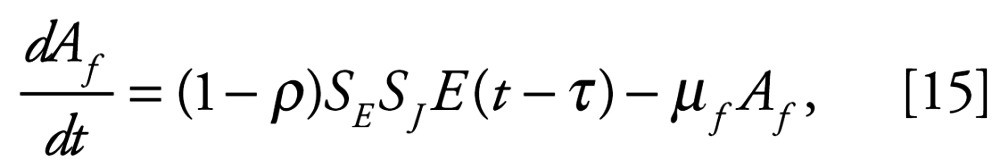
The irreducible minimum of biological detail that our model must encompass is the following: a) adults come in two sexes, one of which produces eggs while the other fertilizes them; b) a fertilized egg takes a finite time (τ) to develop into a reproductively functional adult; c) a proportion, S_J, of eggs will survive this development process: and d) a proportion, ρ, of these survivors become males, whereas the rest become females. The minimal description of the state of a population with these properties is the abundance of adult males and females, which we denote by A_m and A_f , respectively.

One of the more approachable formalisms to describe the dynamics of such a population is that employed by Brown et al. (2003) in modeling the demographic effects of endocrine disruptors in populations of trout, perch, and fathead minnow. Our variant of their description is formulated as a pair of equations that specify the rate of change of A_m and A_f . If we denote the rate of production of fertilized eggs at time t by E(t), and the per-capita mortality rate of male and female adults by μ_m and μ_f , respectively, then the rates of change of A_m and A_f are

and

Model 1: A Well-Mixed Population with No Density Dependence

In this first application of the modeling framework defined by Equations 1 and 2, we make the simplifying assumption that males and females have the same per capita mortality, which we denote by μ (μ_m = μ_f = μ). To complete our population model, we must specify the fertilized egg production rate E. If adult females produce eggs at a per-capita rate β, and the fraction of eggs fertilized at time t is F(t), then

Sperm are less expensive than eggs, so a single male is likely to be capable of fertilizing the reproductive output of many females. If there are no males, then no eggs will be fertilized, while many males will fertilize all released eggs. To model the transition between these limiting cases, we regard the population as well-mixed, so the fraction of eggs fertilized depends on the ratio of males to females, which we denote by

A convenient function relating R and F changes smoothly from 0 to 1 as R increases, and implies that 50% of eggs are fertilized when R = R_h; thus

We note that this formulation implies that essentially all eggs will be fertilized when the male-to-female ratio is large compared with the characteristic value R_h. Also, the proportion fertilized will drop almost linearly with R for values of R that are small compared with R_h. Suppose, for example, that R_h = 0.01. In this case, half the eggs will be fertilized if R = 0.01 (1 male to every 100 females), 90% of eggs will be fertilized if R = 0.1 (1 male to every 10 females), and 98% of eggs will be fertilized if the sex ratio is 1:1.

To understand how the completed model behaves, we differentiate Equation 4, substitute from Equations 1 and 2, and, hence, show that the rate of change R is

Equation 6 demonstrates that after a short transient, the adult male-to-male ratio settles to a steady-state value (which we denote by R^*), given by

and thus is equal to that of the fertilized eggs. This scenario is illustrated by the solid line in Figure 1A.

Figure 1.

A population with no density dependence. (A) The time history of adult female density and adult male-to-female ratio for a population with a 1:1 sex ratio (ρ = 0.5), half-saturation male-to-female ratio R_h = 0.2, juvenile survival S_j = 0.1, and normalized fecundity βτ= 10, initialized with 0.1 females and 0.005 males per unit area. (B) Normalized long-run growth rate, λτ, as a function of BF^*τ with μτ as a parameter. The dotted line shows the boundary between growing and decaying populations (λ= 0).

Once R reaches the steady state (R^*), the rate of change of the adult female population will be given by

where

Because B, F^*, and μ are constants, Equations 7 and 8 tell us that once F has reached F^*, the only possible behaviors this model can exhibit are exponential population growth or decay. Exponential growth is illustrated by the dashed line in Figure 1A.

To calculate the “long-run growth rate” λ, we seek a solution of Equation 8 of the form

and see that such a solution is possible only if λ is a solution of

Although Equation 11 has no closed-form solution, it is still useful. If we multiply both sides by τ, we see that the relation of λ to 1/τ is determined by the two parameter groups BF^*τ and μτ. Equation 11 is also easy to solve numerically, and in Figure 1B we show curves relating λτ to BF^*τ for different values of μτ. A key observation from these curves, which can be confirmed directly from Equation 11, is that a viable population (λ> 0) requires

Model 2: A Well-Mixed Population with Density Dependence

In the last section we saw that a model without appropriate controlling density dependence can predict only exponential growth or decline in the population. To construct a variant of our two-sex population model with a more realistic behavioral repertoire, we assume that survival between egg release and juvenile maturation comprises the following two components: survival from release to hatch, which we denote by S_E, and survival from hatch to maturity, which we denote by S_J. We continue to assume that S_J is a constant, but we imagine that the egg deposition process gets more hazardous as more females become involved. To model this scenario, we assume that egg survival is a decreasing function of adult female abundance (A_f), which we model by writing

thus implying that all fertilized eggs survive to hatch when A_f is very small, 50% survive when A_f = A_h , and none survive when A_f is very large indeed.

The rest of this model variant is essentially the same as before, except that we take the opportunity to relax our previous assumption that adult males and females have the same per-capita mortality rate, by writing

and

where μ_m and μ_f represent the per-capita mortality rates for adult males and females, and the rate of production of fertilized eggs, E, is as before, namely

Unlike the formulation in the previous section, this model has a stationary state in which the ratio of adult male and female populations is given by an expression similar to Equation 7 but reflecting the fact that males and females have differing mortality rates, so that

The steady-state population of adult females is given by

Inspection of Equation 18 shows that for the steady-state population to be positive (i.e., for a biologically meaningful steady state to exist) we require that

In Figure 2A we illustrate the temporal development of a population with density-dependent egg hatching, parameters that satisfy Inequality 19, and an initial male-to-female ratio of 5%. We see that R rapidly attains its stationary value (R^* = 1). While adult abundance is small it exhibits (near) exponential growth. As A_f becomes comparable with A_h, the rate of population growth slows dramatically and the female abundance eventually reaches an asymptote at the value given by Equation 18.

Figure 2.

A population with density-dependent egg hatching. (A) The time history of adult female density and adult male-to-female ratio for a population with ρ = 0.5, R_h = 0.2, μ_fτ = μmτ, S_j = 0.1, βτ = 10, and R_h = 5, intitialized with 0.1 females and 0.005 males per unit area. (B) Normalized steady-state adult female abundance, as a function of BF^* with μ as a parameter.

In Figure 2B we illustrate the dependence of the steady-state adult female abundance on the controlling parameter groups BF^* and μ. For values of BF^* < μ, a viable steady state cannot be established. For BF^* > μ the steady-state adult female abundance increases with BF^* at a rate that depends on μ⁻¹.

Model 3: Temporarily Monogamous Pair Formation

In the last two sections we assumed that the male and female populations are well-mixed, so that any adult male has an equal chance of fertilizing any released eggs. This scenario is clearly inappropriate for many species, so we now investigate an assumption at the opposite end of the spectrum of possibilities, namely, that fish form breeding pairs.

To keep the mathematics simple, and to extend the range of possibilities that the model encompasses, we shall assume that at any instant, the eggs being released by a single female will be fertilized by a single male. At any given instant each male can pair with only one female, so if there is a shortage of males, some females will release unfertilized eggs. Conversely, if there is an excess of males, all females will be paired.

Provided that a single male can fertilize all the eggs released by a single female, and eggs released and not immediately fertilized are permanently infertile, then the proportion of eggs fertilized when the adult male-to-female ratio is R, is

The rest of our model remains unchanged, so the basic dynamics are specified by Equations 14 and 15, and the controlling density dependence is supplied by the adult female dependent hatch probability described by Equation 13. In addition, the fertilized egg production rate is given by Equation 16, and the fertilization fraction is described by Equation 20.

Because it has controlling density dependence, this model will exhibit a stationary state. The analysis leading to Equation 17 carries over unchanged to this model, so we know that at the steady state the adult male-to-female ratio will be as follows:

and the fertilization fraction will be F^* = F(R^*), where F(R) is now specified by Equation 20.

The remaining analysis follows exactly on from that of the last section, yielding the result that

Examination of Equations 20, 21, and 22 shows that if there is an excess of males (R^* > 1), then all released eggs will be fertilized and the steady state depends only on the balance of female fecundity and mortality. If there is an excess of females, their steady-state abundance depends also on the steady-state fertilization fraction, which is just equal to the stationary male-to-female ratio R^*.

Effects of Endocrine Disruptors

The last three sections tell a remarkably consistent story. A model with no limiting density dependence exhibits only exponential growth or decay, whereas one with an appropriately limiting density dependence will eventually approach a steady state. For model 1, which has no limiting density dependence, the ratio of the long-run growth rate λ to the development delay τ is determined by the two parameter groups BF^*τ and μτ. For models 2 and 3, the ratio of the steady-state female abundance to the density dependence parameter A_h is determined by the single parameter group BF^*/μ_f, which represents the number of adult female offspring produced by a single adult female. Our task in this section is to determine how exposure to endocrine disruptors might be expected to change these controlling parameter groups.

Changes in male fecundity and life span

One of the most remarkable effects of exposure to endocrine disruptors is the feminization of male fish (Jobling et al. 1996, 1998). Given a variety of exposure levels within the population described by our model, this phenomenon seems most likely to manifest itself as a reduction in the population average male fecundity, although it is also possible that associated increases in metabolic costs could produce a shortening of adult male life span.

Equations 9, 18, and 22 tell us that the steady-state female abundance predicted by both models with realistic density dependence (models 2 and 3) is influenced only by properties of the adult male subpopulation through the equilibrium proportion of eggs that are fertilized (F^*). Equations 9 and 11 tell us that the same thing applies to the long-run growth rate predicted by model 1.

In models 1 and 2, the equilibrium proportion of eggs fertilized is given by

The effect of a reduction in average male fecundity will be an increase in the adult sex ratio at which 50% fertilization occurs (R_h). A decrease in male life span will be manifested as an increase in the adult male per-capita mortality μ_m, which will result in a decrease in the equilibrium adult sex ratio R^* (Equation 21).

Inspection of Equation 23 shows us that the effect of these changes will be very dependent on the relative values of R^* and R_h. Provided that R^* >> R_h, then F^* will remain close to unity regardless of the actual values of these two quantities. Conversely, if R^* << R_h, then F^* will vary in direct proportion to R^* and in inverse proportion to R_h. We illustrate these two regimes, and the transition between them in Figure 3.

Figure 3.

Steady-state variation with male parameters under model 2. (A) Normalized steady-state abundance of adult females as a function of half-saturation sex ratio (R_h) for a population with R* = 1, and B/μ_f = 4. (B) Normalized steady-state adult female abundance, as a function of μ_m/μ_f for a population with B/μ_f = 4 and R_h = 0.1.

These findings confirm the following conclusion, which is perhaps obvious in retrospect: If there is an excess of males beyond that required to fertilize the entire egg output of the female population, then changes in their number and/or average fecundity will have little effect until a change becomes severe enough to reduce the proportion of fertilized eggs significantly below 1. Because most normal populations will have an equilibrium sex ratio of around 1 and a half-saturation sex ratio between 0.01 and 0.1, R_h or μ_m would need to change by almost an order of magnitude before a significant population-level effect would be observed.

The generality of this conclusion is reinforced by model 3. This model variant assumes that male–female interaction involves individual pair formation, which in turn changes the formula for the fraction of eggs that are fertilized to Equation 20. Within the limiting assumptions of this model (i.e., that a single male is capable of fertilizing the entire reproductive output of his pair), changing male fecundity has no effect on the fraction of eggs fertilized and, hence, on the steady-state population abundance. Inspection of Equation 20 also shows that increasing adult male mortality, and, hence, decreasing the steady–state male/female ratio, does not affect steady-state abundance while R^* remains > 1, after which F^* decreases in proportion to R^*.

Aside from fertilization effects, the properties of all three models we have examined depend only on parameters that characterize the demographic performance of females. Moreover, the effects of changes in these parameters are neither magnified nor ameliorated by the model dynamics. The severity of the resultant demographic effects is therefore dependent on the relative size of the parameter changes induced by the chemical challenge concerned.

A Framework for Modeling Individuals

To provide a systematic way of thinking about the linkage between chemical challenge and changes in demographic performance, we need a model of individual growth, survival, and reproduction. To illustrate the possibilities, we look briefly at a model of female growth and reproduction closely related to a model proposed by Kooijman (1993, 2000).

The model characterizes an individual female by her carbon weight W and asserts that if she assimilates carbon at a rate A, expends a fraction κ of that carbon assimilated on reproduction, and has a basal metabolic expenditure rate M, then her weight must change at a rate given by

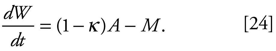Although more detailed variants of this model sometimes have the fractional expenditure on reproduction varying with individual state, we shall only consider its simplest incarnation, in which κ is constant.

We now assume that the maintenance rate M is proportional to the animal’s carbon weight, while the assimilation rate scales with W ^γ, so we write

where the constant ζ represents the weight-specific basal maintenance rate and φ represents the (environment dependent) assimilation scale.

In a constant environment (requiring, at a minimum, constant food availability and constant temperature), the assimilation rate scale φ is independent of time. In this case, provided that γ < 1 (it is normally between 0.6 and 0.8), this model predicts that the individual eventually reaches an asymptotic size (W_∞) that depends on the assimilation rate scale φ (Figure 4A).

Figure 4.

Simple individual growth model. (A) Carbon weight against time for an individual with ζ = 0.09, κ = 0.1 growing in a constant environment, implies a value of φ as marked. (B) Asymptotic fecundity against assimilation scale (φ) with ζ as a parameter for an individual with κ= 0.1.

Examination of Equations 24 and 25 shows that in an environment that makes the assimilation rate scale φ constant, the maintenance cost rate M rises linearly with W, while (so long as γ < 1) the assimilation rate rises with W more slowly. Growth eventually stops when the proportion of assimilation allocated to growth and maintainance, (1 − κ)A, is equal to the rate of expenditure on maintenance, M. This state occurs when W = W_∞, as given by

It is also instructive to calculate the fecundity of a female who has reached her asymptotic weight, which we denote by β_∞. If the carbon cost of an egg is e, then it is quite straightforward to see that β_∞= (κφ/ɛ)(W_∞)^γ. Reference to Equation 26 then shows that

As Figure 4B shows, weight and fecundity at age are sensitively dependent on both the assimilation scale φ and the specific maintenance cost rate ζ.

Individual Effects of Endocrine Disruptors

Except for the more specific and dramatic effects on male sexual function and fertility, endocrine disruptors that are systematically present in modest concentrations seem likely to present a range of effects that have much in common with many other chemical pollutants. Although specific pollutants produce their individual effects through myriad physiological pathways, the most common manifestations of their action at one level of detail below the individual’s demographic performance are increased specific basal metabolic cost (ζ in our model) and decreased assimilation in a given environment (decreased φ in our model).

Before examining the dependence of either growth rate or asymptotic size and fecundity on such changes, it is worth considering the relationship between environment and assimilation scale. The normal form of this dependence is something like

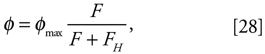where F represents food availability, F_H is the half-saturation food availability (which is related to search volume), and φ_max is the maximum assimilation rate scale (which is related to ingestate handling time).

The effects of an environmental chemical challenge on assimilation can thus manifest themselves either as changes in external activity (search volume) or as changes in internal physiology (handling time). Although changes in φ_max will result in proportional changes in φ, changes in external activity (and, hence, in F_H) will produce significant changes in φ only when food is not in abundance (i.e., when F is not large compared with F_H).

Broadly speaking, chemical challenges seem likely to increase ζ and decrease φ in any given environment. For a species whose individual allometry is such that γ = 0.75, we see from Equation 26 that asymptotic size will change with the ratio (φ/ζ) to the power of 4 and from Equation 27 that asymptotic fecundity will change with 1/ζ to the power of 3 and with φ to the power of 4.

We thus conclude that increases in ζ and decreases in φ_max are unequivocally very bad news indeed, but that reductions in F_H are serious only if food is limiting, or if the decrease is sufficiently large to make it so.

Discussion

In this article we have formulated and analyzed a series of strategic models of populations and individuals subject to challenge by endocrine disruptors. The models are concerned principally with egg-bearing species and neglect special biological features such as parental care. The payoff from this reductionist approach is the simplicity of the resulting models, which has made it possible to obtain useful analytic results by the application of very elementary mathematical methods. The advantage of such methods, where they can be deployed, is that general findings can be obtained much more quickly and definitively than is possible with computational approaches.

Our first investigation examined the demographic importance of alterations to male fertility. Because we sought general results, we took special care to establish not only the generality of our results for a particular model but also their robustness to changes in model structure, representing either uncertainty about basic biological process or variability in process between systems of interest.

Even where the model structure lacks a controlling dependence on density (so that the resulting model can predict only exponential population growth or decay), we were able to show a remarkable consistency of outcome. In all the structural variants we examined, the predicted outcome is controlled by a quantity that can be interpreted as the number of mature female offspring that result from the average female’s lifetime reproductive activity.

This suggests, and our more detailed investigations confirm, that changes in male fertility have little effect at the population level unless the reduction is so general and severe that the chance of released eggs being fertilized is significantly reduced. An adult sex ratio of anything approaching 1:1 guarantees that this reduction in fertilization will happen only when almost all the male population is suffering serious fertility reduction. Hence, we argue that endocrine disruptor exposure will certainly produce deleterious changes in female demographic characteristics at levels much lower than those required to produce population-level effects by altering male fertility.

Our investigation emphasized the importance of identifying those parameters to which population level effects are insensitive, but it also showed that changes in many individual demographic parameters produced population-level changes more or less in proportion to change in the parameter or parameter group concerned.

Even where it is practical to measure individual summary parameters such as fecundity and mortality accurately under realistic exposure conditions, such measurements inevitably occupy a time-span comparable with the lifetime of an individual, which may be many years. By contrast, exposure-induced changes in low-level physiological parameters such as respiration or ingestion rates can be measured on a time scale of days or hours.

Our final demonstration of the utility of simple models therefore examined a strategic model that describes how an individual allocates resources among the three fundamental demographic tasks: growth, maintenance, and reproduction. We showed that the techniques that yield good biological gain for low mathematical pain in the context of population dynamic models also work when applied to models that describe individual energy budgets. Thus, we have provided a viable route for investigating the sensitivity of an individual’s demographic summary parameters to changes in low-level physiological rates.

References

Footnotes
This article is part of the monograph “The Ecological Relevance of Chemically Induced Endocrine Disruption in Wildlife.”
- Brown AR, Riddle AM, Cunningham NL, Kedwards TJ, Shillabeer N, Hutchinson TH. Predicting the effects of endocrine-disrupting chemicals on fish populations. Hum Ecol Risk Assess. 2003;9(3):761–788. [Google Scholar]
- Jobling S, Beresford N, Nolan M, Rodgers-Gray R, Tyler CR, Sumpter JP. Altered sexual maturation and gamete production in wild roach (Rutilus rutilus) living in rivers that receive treated sewage effluents. Biol Reprod. 2002;66:272–281. doi: 10.1095/biolreprod66.2.272. [DOI] [PubMed] [Google Scholar]
- Jobling S, Nolan M, Tyler CR, Brighty G, Sumpter J. Widespread sexual disruption in wild fish. Environ Sci Tech. 1998;32:2498–2506. doi: 10.1289/ehp.8050. [DOI] [PMC free article] [PubMed] [Google Scholar]
- Jobling S, Sheahan D, Osborne J, Mattheisen P, Sumpter J. Inhibition of testicular growth in rainbow trout (Oncorhynchus mykiss) exposed to estrogenic alkylphenolic chemicals. EnvironToxicol Chem. 1996;15:194–202. [Google Scholar]
- Kooijman SALM. 1993. Dynamic Energy Budgets in Biological Systems. Cambridge, UK:Cambridge University Press.
- Kooijman SALM. 2000. Dynamic Energy and Mass Budgets in Biological Systems. Cambridge, UK:Cambridge University Press.
- Panter GH, Thomson RS, Sumpter JP. Adverse reproductive effects in male fathead minnows (Pimephales promelas) exposed to environmentally relevant concentrations of the natural oestrogens oestradiol and oestrone. Aqua Toxicol. 1998;42:243–253. [Google Scholar]
- Van Winkle W, Rose KA, Chambers RC. Individual-based approach to fish population dynamics—a review. Trans Am Fish Soc. 1993;380:397–403. [Google Scholar]