Improving comparability between microarray probe signals by thermodynamic intensity correction

Abstract

Signals from different oligonucleotide probes against the same target show great variation in intensities. However, detection of differences along a sequence e.g. to reveal intron/exon architecture, transcription boundary as well as simple absent/present calls depends on comparisons between different probes. It is therefore of great interest to correct for the variation between probes. Much of this variation is sequence dependent. We demonstrate that a thermodynamic model for hybridization of either DNA or RNA to a DNA microarray, which takes the sequence-dependent probe affinities into account significantly reduces the signal fluctuation between probes targeting the same gene transcript. For a test set of tightly tiled yeast genes, the model reduces the variance by up to a factor ∼1/3. As a consequence of this reduction, the model is shown to yield a more accurate determination of transcription start sites for a subset of yeast genes. In another application, we identify present/absent calls for probes hybridized to the sequenced Escherichia coli strain O157:H7 EDL933. The model improves the correct calls from 85 to 95% relative to raw intensity measures. The model thus makes applications which depend on comparisons between probes aimed at different sections of the same target more reliable.

INTRODUCTION

Signals from oligonucleotide microarrays have proven highly reproducible and the great majority of the stochastic variation seen typically originates from differences in the samples measured. The high reproducibility of the signal, however, breaks down when signals from different probes, targeted against the same target, are compared (1,2). Hence, probes measuring the same gene transcript, in the same sample, present on the same oligonucleotide array, typically result in a wide range of signal intensities. The microarray community have in large avoided this problem by restricting comparisons to be between identical probes. Even where multiple probes are targeted against a given transcript, the comparisons are done probe wise (3) or they are based on so-called expression index calculations (1,4) that carefully avoid comparisons across different probes. Comparisons between different probes, however, are of great interest because they allow detection of differences along a sequence. Microarray detection of intron/exon architecture, transcription boundary, the methylation state of genomic regions, etc. depends on such comparisons. Ultimately, probe comparisons will allow absent/present calls. Substantial amounts of data using tiling arrays are available (5–7) as well as data on exon/intron detection (8). At present, analyses hereof have relied on statistical or rule-based approaches, exploiting the continuation of the signal levels along a sequence or elevated signal within a window (5,6). The relative high signal variation between probes restricts such methods from detecting short stretches of shuttle differences. Importantly, much of the probe variation is sequence dependent (9). Hence, correcting for the sequence-dependent variation among probes should compensate for the intensity fluctuations of probes targeting the same gene.

Here we present a thermodynamic model for the microarray hybridization, taking the sequence-dependent hybridization affinities into account. We use the model to analyze two different microarray experiments: one based on DNA–RNA hybridization and one based on DNA–DNA hybridization. The main purpose of the present article is to demonstrate how such a model can be used to improve the analysis of experiments which rely on comparisons between individual probes aimed at different sections of the same target. This is because the model takes into account the different binding affinities of the probes thereby compensating partially for the signal intensity fluctuations of probes with the same target. The model thus has the important advantage that it allows a more quantitative comparisons between signals from different probes. We describe two applications of this. First, we use the model to determine the position of transcriptions start sites (TSS) with greater accuracy than is possible using the raw signals. We then use the model to identify the presence/absence of DNA segments in a cross-strain DNA hybridization between two sequenced Escherichia coli strains. Again, the model yields significantly more reliable results than when using the raw intensities.

MATERIALS AND METHODS

Array design

The genome sequence for Sacchoromyces cerevisiae was downloaded from the SGD FTP site (ftp://genome-ftp.stanford.edu/pub/yeast/), on the 18th of September 2004, and all CDSs were extracted (DNA and Intron/Exon annotation), using the FeatureExtract software (10). Using this sequence information as a basis, the following probe-sets were designed: Up to 20 probes per gene for S. cerevisiae genes (n = 5866) were selected using OligoWiz 2 (11,12). In addition to the exon probes, probes with a minimum distance of 25 bp were placed targeting the regions 300 bp upsteam and 100 bp downsteam of each gene (using OligoWiz 2).

About 5000 random probes of length 25 bp where generated, using 25% probability of each of the four nucleotides: A, T, G and C.

About 28 genes (12 of these in duplicate, yielding 40 in total) covering the range from low to high expression, according to de Lichtenberg et al. (13) were densely tiled with probes (see table below). 23, 25 and 27 bp probes were designed, with 10 bp between the midpoints of the probes. This means all three length-variants of the probes are centered on the same position. In total 18 759 tiling probes were designed for each of the three probe lengths, 23, 25 and 27 bp. The data can be found at http://www.cbs.dtu.dk/suppl/probes/.

Systematic name	Standard name	In duplicate	Gene length	No. of probes
YAR007C	RFA1	X	1866	185
YAR071W	PHO11	X	1404	138
YBL002W	HTB2	X	396	38
YBR093C	PHO5	X	1404	138
YBR243C	ALG7	X	1347	266
YCL014W	BUD3		4911	489
YDL003W	MCD1		1701	168
YDL224C	WHI4		1950	193
YER001W	MNN1	X	2289	227
YGR044C	RME1		903	88
YGR108W	CLB1	X	1416	140
YHR086W	NAM8		1572	155
YHR175W	CTR2		570	55
YIL132C	CSM2		642	62
YIR018W	YAP5		738	72
YJL092W	HPR5	X	3525	351
YKR042W	UTH1		1353	133
YLR353W	BUD8		1812	179
YMR042W	ARG80	X	534	51
YMR215W	GAS3	X	1575	156
YMR305C	SCW10		1170	115
YNL176C			1911	189
YOR070C	GYP1		1914	189
YOR144C	ELG1		2376	236
YPL128C	TBF1	X	1689	167
YPL163C	SVS1	X	783	76
YPL208W	RKM1		1752	173
YPL256C	CLN2		1638	162

Experimental procedures

The RNA used in the experimental part of this publication, was extracted from a S. cerevisiae CDC15-2 strain 30 min after release from a temperature induced arrest of the cell cycle in late mitotic phase. See (13) for strain and growth condition details. Total RNA was extracted using the FastRNA pro red kit from Qbiogene, according to the manufacturers description—for the lysis step the samples were processed for 40 s at speed 6.0 in the FastPrep apparatus. Quality and quantity of total RNA was assessed using spectrophotometer readings at 260 and 280 nm and using an Agilent Bioanalyzer. aRNA was synthesized using the Message Amp II Biotin Enhanced kit (Ambion), using oligo-dT primers, and aRNA fragmentation was done by heating the aRNA to 94°C for 35 min in a MgCl₂ buffer. Hybridization was performed according to the standard Affymetrix protocol. Raw probe intensity values for our custom-designed NimbleExpress chip were obtained using the makecdfenv and affy packages from Bioconductor (14).

Intensities were taken from whole chromosomal DNA hybridizations of E. coli strain O157:H7 EDL933 (15,16) and K-12 W3110 (17) to custom-designed NimbleExpress arrays covering seven E. coli genomes including EDL933 and W3110 (18). In short, independent biological triplicates of each strain were grown overnight in Luria–Bertani (LB) broth with continuous agitation (19), and DNA was isolated using the Qiagen Genomic Tip 500/G (Qiagen, Hilden, Germany) and the Genomic DNA Buffer set (Qiagen). Seven microgram of genomic DNA was fragmented with 0.7 Units of DNAse 1 (Amersham Biosciences, Piscateway, NJ) for 10–12 min at 37°C in 1× One-Phor All Plus buffer (Amersham Biosciences) to obtain fragments of 50–200 bp. Fragmented DNA was labeled according to the manufacturers instructions for labeling fragmented cDNA derived from mRNA for prokaryotic arrays (Affymetrix Inc., Santa Clara, CA). The labeled DNA was hybridized to custom made NimbleExpress arrays (Affymetrix Inc.) for 15–17 h at 45°C. Standard protocols from Affymetrix for hybridization, washing and staining were followed using a hybridization oven, a Fluidics Station 450 and a GeneChip® Scanner 3000 (Affymetrix Inc.). Custom-designed probes were mapped to the EDL933 and W3110 genomes for which probes were included on the array. Hereby, we could determine to which extend W3110 probes theoretically should hybridize to the EDL933 samples and vice versa.

Physicochemical model

The results presented in this article are based on a physical model for the binding of fluorescently labeled RNA/DNA strands to the oligonucleotides on the DNA chip. The model is similar to the ones presented in Ref. (9,20–22). It is based on equilibrium thermodynamics and assumes that the observed intensity variations between probes for the same gene are due to differences in the binding energies between the probes and the RNA/DNA strands. The model applies to both RNA and DNA strands in solution but we will for brevity refer to the case of RNA strands in the rest of this section. For DNA strands, the model is completely analogous. For simplicity, the model neglects effects such as secondary structures and cross-hybridization and assumes that a given probe is either completely bound to one RNA strand or unbound (free). The basic process for the probe-RNA hybridization is

1

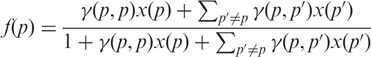
The binding of RNA strands to a given probe can be split into two types: Specific binding for which the probe is bound to its complimentary (target) RNA strand, and non-specific binding for which the probe is bound to an RNA strand which is not its complimentary. Let x(p) be the concentration of RNA strands of type p. If f(p) ∈ [0,1] denotes the fraction of probes with target RNA of type p which are bound to a RNA strand, equilibrium thermodynamics predicts (23)

2

where γ (p,p′) is the equilibrium constant for the binding of RNA strands of type p′ to a probe for target RNA p. In Equation (2), we separate the specific binding process explicitly from the non-specific ones: The term γ (p,p)x(p) describes the specific binding whereas the term ∑_{p′ ≠ p} γ (p,p′)x(p′) describes the non-specific binding. For a well-designed probe, the specific binding is expected to be dominant and γ (p,p) ≫ γ (p,p′) with p′ ≠ p. The equilibrium constants are given by (23)

3

where Δ G(p,p′) is the Gibbs free energy difference for the binding process for RNA strands of type p′ to probes for target RNA p with T the temperature. The free energies must be expected to depend strongly on the base sequence of the probe/target RNA.

The observed intensity I(p) for a given probe is proportional to the fraction of probes f(p) bound to a RNA strand, i.e. I(p) = κ f(P). We can rewrite Equation (2) as

4

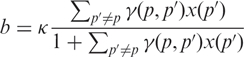
Here, the term b(p) yields the intensity coming from non-specific binding. It is given by

5

as can be obtained from Equation (2) by putting the target RNA concentration to zero, x(p) = 0. Likewise, the first term in Equation (4) yields the intensity coming from specific binding with the parameters a(p) and c(p) given in terms of the equilibrium constants in Equation (2). The intensity saturates at I = c + b when x → ∞. This limit corresponds to all the probes bound to their target RNA for very high target concentration.

A major goal for a model for the hybridization process on DNA chips is to yield information on the concentration of the RNA strands in the solution. This is given by the inverse of Equation (4):

6

Model for probe intensity parameters

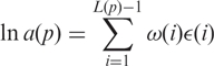
To proceed, we need a model for how the parameters a(p), b(p) and c(p) depend on the probe sequence. We will use a position dependent nearest neighbor model to describe the dependence of the hybridization energies on the probe sequence writing

7

and likewise for b(p) and c(p). Here, i denotes the base-pair position along the probe of length L bases, ω(i) is the position-dependent weight function, and ε (i) = ε_AA, ε_AT,…, ε_GG depending on whether the base pair at position i and i + 1 is AA, AT,…, GG. The model thus assumes that the binding energy for the hybridization is a sum of the binding energies ε_XX between base pairs along the probe. We have introduced a function ω(i) to describe a position dependence of the binding energy between base pairs. This position dependence can be due to steric effects coming from the presence of the chip surface. There are three sets of independent fitting parameters ε_XX and ω(i) corresponding to the three parameters a(p), b(p) and c(p). In the following, we refer to this position-dependent model as the ‘PD’ model.

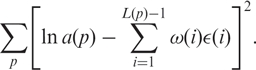
The fitting procedure is based on the least squares method. For instance, to find the ε_XX and ω(i) parameters for a(p) we minimize

8

The fitting procedure for the parameters b(p) and c(p) is identical. The parameters a(p), b(p) and c(p) are found by a least squares fitting of the observed intensities to the Langmuir form (4). More details of the fitting procedure can be found in the supplementary notes.

In the supplementary notes, the accuracy of the model is established by benchmarking it using the Affymetrix Spike-In U95 data set (24) and comparing it to other models in the literature (22,25–27).

RESULTS

Fluctuation reduction between probes of the same target

The main goal of the present article is to enable a more reliable comparison between intensity data coming from probes targeting different sections of the same target. In this section, we therefore analyze the models ability to correct for fluctuations between probes targeted against the same gene transcript. An oligonucleotide microarray holding probes densely tiling 28 yeast genes, were hybridized (for details see Materials and methods, Array design section). Here, we analyze the data from the resulting 18 759 tiling probes targeting 28 genes with unknown concentration in the yeast data set. We write for probes which target a RNA sequence from a gene . The intensities I(p) vary strongly within this probe set even though they probe the same gene. Since we in the yeast experiment do not have (as opposed to the Spike-In data) intensity data for the same probes at different known target concentrations, we cannot use the full non-linear Langmuir form Equation (4). We therefore linearize Equation (4) obtaining

9

This linearization corresponds to assuming a non-saturating concentration x(p) of the RNA fragments in the yeast experiment. The probe dependence of the background intensity b(p) is known from the random probe analysis (see supplementary notes). For probes , the concentration x(p) is constant and the right-hand side of Equation (9) only depends on the probe sequence through c(p)/a(p). In analogy with the Spike-In analysis (see supplementary notes), we therefore fit (least squares) the observed intensity from probes to the PD model using Equation (7) with ln a(p) replaced by ln [c(p)x(p)/a(p)]. To minimize the uncertainty for the fitting parameters, we pick the gene targeted by the most probes (489 probes). The result of the fit is shown in Figure 1a. Here, we have plotted the observed intensities and the prediction of the fit for probes . For clarity, we plot only the first 100 of the 489 probes in the plot. As we see from Figure 1a, the model describes the main features of the hybridization of the probes.

Figure 1.

(a) The observed raw intensities from probes targeting the tiling gene used for fitting (black ×) and the predictions of the PD fit (red □) as a function of probe position along the gene. (b) The observed raw intensities from probes targeting a tiling gene not used for fitting and the predictions of the PD fit.

With the fitting parameters determining the probe sequence dependence of ln [c(p)x(p)/ a(p)] for probes [with constant x(p)] obtained, one can use Equation (9) to predict the concentration of other genes relative to . We rewrite Equation (9) for a probe p′ probing RNA strands from gene () with unknown concentration x(p′) as

10

Given the base sequence for probe p′, ln [c(p′)x(p)/a(p′)] predicts a value for the observed intensity assuming the product of target gene has the same concentration as the product of the gene used for the fitting of Equation (9), i.e. x(p′) = x(p). The difference between the prediction of the fit and the observed intensity should be constant for all probes targeting a given gene product and yields from Equation (10) the relative concentration of gene product compared to . To illustrate this, we plot in Figure 1b the observed intensity from probes targeting a gene transcript and the model prediction for the intensity given the probe sequence. Again, we only show the first ∼ 100 probes. We see that the model prediction for the intensity is consistently lower than the observed intensity. From Equation (10), this corresponds to a higher concentration of gene product as compared to gene product . Furthermore, the difference between the observed intensity and the prediction is approximately constant in agreement with Equation (10). By performing a probe average of this difference for probes , we obtain from Equation (10) an estimate of the concentration of gene product relative to . We denote this by . For the specific gene plotted in Figure 1b, we obtain , i.e. the concentration of gene is 7.6 times higher than . Using this approach, one can obtain the concentration of all the gene products not used for fitting relative to the gene product used for fitting.

As stated above, a major purpose of our theory is to explain the large variations in the raw intensity between probes targeting the same gene. To illustrate this variation, we present in Figure 2 a box plot of the intensities for probes targeting a given gene not used for determining the fitting parameters. A box plot of the corresponding predicted concentration obtained from the PD model is also shown. We see that variation of the concentration predictions is significantly lower than for the raw intensities. For the specific gene in Figure 2, we have Var[log (x)]/Var[log (I)] = 0.34; the variation of the signal from the probes targeting the same gene is reduced by a factor ∼ 3. Averaging the variation over all the genes, we obtain

11

The model thus is able to compensate partially for the variation of the observed intensity thereby reducing the uncertainty in the predicted concentration of the gene. For a perfectly working model there would be no variation in the predicted concentration. There is of course still a residual variation for the predicted concentration which is to be expected as our rather simple model cannot describe all the complicating effects in the hybridization process and in the experimental procedure.

Figure 2.

Box plot of the observed intensities from probes targeting a given gene and of the corresponding concentrations obtained from the PD model.

A way to improve the performance of the model could be to add random probes with the same base-pair content as the probes targeting the yeast genomes. Providing one can neglect the position dependence of the binding process, such probes would give more information on the background (non-specific) binding contribution to the signal which could be used by our model.

Application: determining TSS from probe signals

One of the main motivations for this work is to facilitate a present/absent call as well as to decide the boundary of transcripts along a genomic sequence through hybridization of probes targeted along a genome sequence.

Since the RNA is not expressed from regions upstream of the transcription start sites (TSS), there is no specific binding to probes targeting these regions. Consequently, we expect the intensity of such probes to be smaller than those targeting the transcribed regions. However, this tendency is often distorted by the large variations in the observed intensity due to affinity differences between probes. As demonstrated above, the physicochemical model presented in this article can partially compensate for these variations.

The approach is as follows. We use Equation (10) to extract RNA concentrations relative to the tiled gene for which the model was fitted. We then fit both the observed intensity and the corresponding predicted concentrations [using Equation (10)] from probes around an expected TSS to the functional form

12

with x₀, Δ x, r₀ and Δ r fitting parameters. Here x_r denotes the concentration of transcript starting at base position r along the gene. The parameter x₀ gives an offset, Δ x gives the change in the concentration across the gene start/end position, r₀ is the fitted value for the position of the gene start/end position and Δ r is the width of the position (the uncertainty). We expect Δ r to be of the order of the probe lengths, as we cannot determine the gene start/end position with greater accuracy than the base length of the probes used. We analyzed intensities from probes of length 27 bases. Note that we need the parameter x₀ since the genes in general have a different concentration than the tiling gene used for the fitting giving rise to an offset as explained above. The observed intensities are fitted to the same functional form (12).

To illustrate the performance of the model, we show in Figures 3 and 4 two examples of such a fit to a TSS. In both cases, the translation start is at base position 0. For both TSSs, the fluctuations of the observed intensities (Figures 3a and 4a) are rather large making a precise determination of the gene start position difficult. The fit based on Equation (12) for the raw intensities yields χ²/(N−4) = 1.3 for TSS1 and χ²/(N−4) = 1.8 for TSS2 where N is the number of intensities used in the fit and we subtract 4 since there are four fitting parameters. Figures 3b and 4b show the corresponding fits on the predicted concentration profiles obtained from Equation (10). For the TSS1 shown in Figure 3b, the model works very well in reducing the fluctuations of the signal. There is a clearer change in the predicted concentrations for probes around the gene start position and the fit based on Equation (12) is much better with χ²/(N−4) = 0.033. For the TSS2 shown in Figure 4b, the model also reduces the fluctuations albeit less effectively. The reduction in the fluctuations results in a better fit to Equation (12) with a reduced χ²/(N−4) = 1.0 as compared to when the raw intensities are used.

Figure 3.

TSS1: (a) The observed intensities as a function of probe position along the gene. (b) The corresponding predicted to concentration from Equation (10). The lines are fits based on Equation (12). Zero marks the translation start (SGD-REF).

Figure 4.

TSS2: Same as for Figure 3.

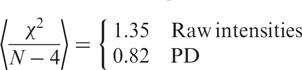
In total, 529 TSS where analyzed. Including probes positioned ± 300 base positions around the gene translational-start positions, we obtain an average χ

13

when fitting the intensities and the thermodynamic models to Equation (12). From Equation (13), we conclude that the PD model allows for a more reliable determination of the location of the TSS.

Absent/present call on DNA–DNA hybridization

We now analyze the microarray data from genomic DNA hybridizations of E. coli O157:H7 EDL933 to a custom-designed microarray covering seven E. coli genomes including the K-12 W3110 strain. By mapping to the known sequence of W3110, we identified probes that should hybridize to the EDL933 sample, in theory. These probes experience specific binding to their target DNA strands and we denote them as present-probes. The rest of the probes in general have a lower intensity since they do not experience specific binding; we denote them absent-probes. This is illustrated in Figure 5a. However, as we see from the figure, the intensity of the present- and absent-probes exhibit large fluctuations and their intensity distributions partly overlap. This complicates the identification of present-/absent-probes based on the raw intensities from the microarray experiment. By defining probes with an intensity above a certain threshold as on and probes below as absent, we will incorrectly identify a number of absent-probes as present (false positive) and vice versa.

Figure 5.

(a) The total raw intensity distribution and the distribution of present-/absent-probes. (b) The corresponding corrected intensities (plus an offset to adjust to the same mean value as for the intensities).

The present model compensates partially for these fluctuations yielding more narrow distributions for the present-/absent-probes with less overlap. This is illustrated in Figure 5b. Here, we have taken a subset of the absent-probes whose signal exclusively comes from non-specific binding and fitted (least squares) the observed signal ln I(p) = ln b(p) to the model (7) with a(p) replaced by b(p). We then compensate the signal from the rest of the probes by subtracting the predicted background signal from the probe, i.e. the corrected intensity is ln I(p) − ln b(p) with ln b(p) given by Equation (7). In this way, we partially compensate for the fluctuations in the data coming from the non-specific binding thereby allowing a more accurate identification of present-/absent-probes. Note that we do not train the model on a subset of the present-probes also. This is because we want to test the ability of the model to predict with no prior knowledge whether a probe is present or absent. Our procedure corresponds to assuming that the one can train the model on a set of probes which are known not to target any present targets. The model is then applied to a set of probes where it is unknown whether they are present or absent.

In Figure 6, we plot the receiver operating characteristic (ROC) curves (fraction true positive versus fraction false positive, at varying thresholds) for both the raw and the corrected probe signals. We see that the area under the ROC curve is significantly larger for corrected probe intensities resulting in 95% versus 85% correctly classified probes at the optimal threshold for the corrected and raw signals, respectively. Thus, we conclude that the model indeed allows a more reliable identification of present-/absent-probes.

Figure 6.

ROC curves based on the raw intensities and the PD model for the concentrations.

DISCUSSION

DNA microarray hybridization signals are distorted by various factors. A significant part of the distortion can be attributed to the base sequence dependence of the probe affinity. We presented a physicochemical theory for the hybridization process on microarrays using a position dependent nearest neighbor model for the binding energies. In this way, we take stacking energies and positional effects within the probes into account when analyzing the hybridization signal.

The main purpose of the article is to demonstrate that such a model allows the signals from different probes with the same target to be compared more accurately, as the conversion renders the signal less dependent on the probe affinity. We demonstrated that the model reduces the signal variance up to 64\ % for probes with the same target. It thus enables a more quantitative comparison of signals from different probes. Two applications of this were presented.

First, we demonstrated that our model provides a more accurate estimate of the position of TSS as compared to using raw intensities. The probe data were fitted to a hyperbolic tangent to model the TSS. Not surprisingly, the reduction in the signal variation by our model improves the fit significantly. This result does not depend on the specific functional form (hyperbolic tangent) used for the fit; others may want to model the TSS, other part of the gene structures or absence of transcription all together, by other means. We expect that most methods should benefit from using signals corrected for probe affinity effects by thermodynamic intensity correction similar to the one presented here.

Second, as a benchmark for ability of the model to separate signal from no signal, commonly referred to as absent/present call, we turned to a data set where the result is known a priory. Genomic DNA from the E. coli strain EDL933 for which the genomic sequence have previously been determined, was hybridized to a microarray containing probes for another E. coli strain, namely W3110. The correct call (absent/present) could be determined for 85\% of the probes when the raw signals were used, whereas 95\% correct calls could be made when using probe affinity corrected signals. This demonstrated a very useful application of our model. Also, it shows that the model works for DNA–DNA hybridization as well as RNA–DNA hybridization.

A software implementation of the model presented in this article together with a description on how to use it is available at http://www.cbs.dtu.dk/suppl/probes/. In the future, one could improve the performance of the model even further by taking into account additional aspects of the hybridization such as probe and/or target folding and sandwich hybridization.

SUPPLEMENTARY DATA

Supplementary Data is available at NAR online.

REFERENCES

- 1.Li C, Wong WH. Model-based analysis of oligonucleotide arrays: expression index computation and outlier detection. Proc. Natl. Acad. Sci. USA. 2001;98:31–36. doi: 10.1073/pnas.011404098. [DOI] [PMC free article] [PubMed] [Google Scholar]
- 2.Irizarry RA, Hobbs B, Collin F, Beazer-Barclay YD, Antonellis KJ, Scherf U, Speed TP. Exploration, normalization, and summaries of high density oligonucleotide array probe level data. Biostatistics. 2003;4:249–264. doi: 10.1093/biostatistics/4.2.249. [DOI] [PubMed] [Google Scholar]
- 3.Lemon WJ, Liyanarachchi S, You M. A high performance test of differential gene expression for oligonucleotide arrays. Genome Biol. 2003;4:R67. doi: 10.1186/gb-2003-4-10-r67. [DOI] [PMC free article] [PubMed] [Google Scholar]
- 4.Irizarry RA, Bolstad BM, Collin F, Cope LM, Hobbs B, Speed TP. Summaries of Affymetrix GeneChip probe level data. Nucleic Acids Res. 2003;31:e15. doi: 10.1093/nar/gng015. [DOI] [PMC free article] [PubMed] [Google Scholar]
- 5.Shoemaker DD, Schadt EE, Armour CD, He YD, Garrett-Engele P, McDonagh PD, Loerch PM, Leonardson A, Lum PY, et al. Experimental annotation of the human genome using microarray technology. Nature. 2001;409:922–927. doi: 10.1038/35057141. [DOI] [PubMed] [Google Scholar]
- 6.Stolc V, Samanta MP, Tongprasit W, Sethi H, Liang S, Nelson DC, Hegeman A, Nelson C, Rancour D, et al. Identification of transcribed sequences in Arabidopsis thaliana by using high-resolution genome tiling arrays. Proc. Natl. Acad. Sci. USA. 2005;102:4453–4458. doi: 10.1073/pnas.0408203102. [DOI] [PMC free article] [PubMed] [Google Scholar]
- 7.Cheng J, Kapranov P, Drenkow J, Dike S, Brubaker S, Patel S, Long J, Stern D, Tammana H, et al. Transcriptional maps of 10 human chromosomes at 5 nucleotide resolution. Science. 2005;308:1149–1154. doi: 10.1126/science.1108625. [DOI] [PubMed] [Google Scholar]
- 8.Clark TA, Sugnet CW, Ares M., Jr Genomewide analysis of mRNA processing in yeast using splicing-specific microarrays. Science. 2002;296:907–910. doi: 10.1126/science.1069415. [DOI] [PubMed] [Google Scholar]
- 9.Binder H, Kirsten T, Loeffler M, Stadler PF. Sensitivity of microarray oligonucleotide probes: variability and effect of base composition. J. Phys. Chem. B. 2004;108:18003. Binder,H., Kirsten,T., Hofacker,I.L., Stadler,P.F. Loeffler,M. (2004) Interactions in oligonucleotide hybrid duplexes on microarrays. J. Phys. Chem. B, 108, 18015. [Google Scholar]
- 10.Wernersson R. FeatureExtract–extraction of sequence annotation made easy. Nucleic Acids Res. 2005;33:W567–W569. doi: 10.1093/nar/gki388. [DOI] [PMC free article] [PubMed] [Google Scholar]
- 11.Wernersson R, Nielsen HB. OligoWiz 2.0–integrating sequence feature annotation into the design of microarray probes. Nucleic Acids Res. 2005;33:W611–W615. doi: 10.1093/nar/gki399. [DOI] [PMC free article] [PubMed] [Google Scholar]
- 12.Nielsen HB, Wernersson R, Knudsen S. Design of oligonucleotides for microarrays and perspectives for design of multi-transcriptome arrays. Nucleic Acids Res. 2003;31:3491–3496. doi: 10.1093/nar/gkg622. [DOI] [PMC free article] [PubMed] [Google Scholar]
- 13.de Lichtenberg U, Wernersson R, Jensen TS, Nielsen HB, Fausboll A, Schmidt P, Hansen FB, Knudsen S, Brunak S. New weakly expressed cell cycle-regulated genes in yeast. Yeast. 2005;22:1191–1201. doi: 10.1002/yea.1302. [DOI] [PubMed] [Google Scholar]
- 14.Gautier L, Cope L, Bolstad BM, Irizarry RA. Affy–analysis of Affymetrix GeneChip data at the probe level. Bioinformatics. 2004;20:307–315. doi: 10.1093/bioinformatics/btg405. [DOI] [PubMed] [Google Scholar]
- 15.O'Brien AD, Newland JW, Miller SF, Holmes RK, Smith HW, Formal SB. Shiga-like toxin-converting phages from Escherichia coli strains that cause hemorrhagic colitis or infantile diarrhea. Science. 1984;226:694–696. doi: 10.1126/science.6387911. [DOI] [PubMed] [Google Scholar]
- 16.Perna NT, Plunkett G, III, Burland V, Mau B, Glasner JD, Rose DJ, Mayhew GF, Evans PS, Gregor J, et al. Genome sequence of enterohaemorrhagic Escherichia oli O157:H7. Nature. 2001;409:529–533. doi: 10.1038/35054089. [DOI] [PubMed] [Google Scholar]
- 17.Hayashi K, Morooka N, Yamamoto Y, Fujita K, Isono K, Choi S, Ohtsubo E, Baba T, Wanner BL, et al. Highly accurate genome sequences of Escherichia coli K-12 strains MG1655 and W3110. Mol. Syst. Biol. 2006;2 doi: 10.1038/msb4100049. 2006.0007. [DOI] [PMC free article] [PubMed] [Google Scholar]
- 18.Willenbrock H, Petersen A, Sekse C, Kiil K, Wasteson Y, Ussery DW. Design of a 7 Escherichia coli Genomes Microarray for Comparative Genomic Profiling. J. Bacterio. 2006;188:7713–7721. doi: 10.1128/JB.01043-06. The data is available from the Gene Expression Omnibus database (GEO: http://www.ncbi.nlm.nih.gov/geo/) with the series accession number GSE4690. [DOI] [PMC free article] [PubMed] [Google Scholar]
- 19.Sambrook J, Fritsch EF, Maniatis T. Molecular Cloning: A Laboratory Manual. 2nd ed. Cold Spring Harbor, NY: Cold Spring Harbor Laboratory Press; 1989. [Google Scholar]
- 20.Held GA, Grinstein G, Tu Y. Modeling of DNA microarray data by using physical properties of hybridization. PNAS. 2003;100:7575. doi: 10.1073/pnas.0832500100. [DOI] [PMC free article] [PubMed] [Google Scholar]
- 21.Held GA, Grinstein G, Tu Y. Relationship between gene expression and observed intensities in DNA microarrays – a modeling study. Nucleic Acids Res. 2006;34:e70. doi: 10.1093/nar/gkl122. [DOI] [PMC free article] [PubMed] [Google Scholar]
- 22.Hekstra D, Taussig AR, Magnasco M, Naef F. Absolute mRNA concentrations from sequence-specific calibration of oligonucleotide arrays. Nucleic Acids Res. 2003;31:1962. doi: 10.1093/nar/gkg283. [DOI] [PMC free article] [PubMed] [Google Scholar]
- 23.Silbey RJ, Alberty RA. Physical Chemistry. West Sussex, UK: John Wiley; 2000. [Google Scholar]
- 24. Available from http://www.netaffx.com.
- 25.Zhang L, Miles MF, Aldape FD. A model of molecular interactions on short oligonucleotide microarrays. Nature Biotechnol. 2003;21:818. doi: 10.1038/nbt836. [DOI] [PubMed] [Google Scholar]
- 26.Wu Z, Irizarry RA, Gentleman R, Martinez-Murillo F, Spencer F. A model based background adjustment for oligonucleotide expression arrays in the journal of the american statistical association. 2004;99:909. [Google Scholar]
- 27.Wu Z, Irizarry RA. Nat. Biotechnol. 2004;22:656. doi: 10.1038/nbt0604-656b. [DOI] [PubMed] [Google Scholar]
- 28.Choe1 SE, Boutros M, Michelson AM, Church GM, Halfon MS. Preferred analysis methods for Affymetrix GeneChips revealed by a wholly defined control dataset. Genome Biol. 2005;6:R16. doi: 10.1186/gb-2005-6-2-r16. [DOI] [PMC free article] [PubMed] [Google Scholar]