From Single-Cell Genetic Architecture to Cell Population Dynamics: Quantitatively Decomposing the Effects of Different Population Heterogeneity Sources for a Genetic Network with Positive Feedback Architecture

Abstract

Phenotypic cell-to-cell variability or cell population heterogeneity originates from two fundamentally different sources: unequal partitioning of cellular material at cell division and stochastic fluctuations associated with intracellular reactions. We developed a mathematical and computational framework that can quantitatively isolate both heterogeneity sources and applied it to a genetic network with positive feedback architecture. The framework consists of three vastly different mathematical formulations: a), a continuum model, which completely neglects population heterogeneity; b), a deterministic cell population balance model, which accounts for population heterogeneity originating only from unequal partitioning at cell division; and c), a fully stochastic model accommodating both sources of population heterogeneity. The framework enables the quantitative decomposition of the effects of the different population heterogeneity sources on system behavior. Our results indicate the importance of cell population heterogeneity in accurately predicting even average population properties. Moreover, we find that unequal partitioning at cell division and sharp division rates shrink the region of the parameter space where the population exhibits bistable behavior, a characteristic feature of networks with positive feedback architecture. In addition, intrinsic noise at the single-cell level due to slow operator fluctuations and small numbers of molecules further contributes toward the shrinkage of the bistability regime at the cell population level. Finally, the effect of intrinsic noise at the cell population level was found to be markedly different than at the single-cell level, emphasizing the importance of simulating entire cell populations and not just individual cells to understand the complex interplay between single-cell genetic architecture and behavior at the cell population level.

INTRODUCTION

Biological complexity originates from various sources. First, the DNA of organisms is comprised of a large number of genes, which, depending on the intracellular state, might be on or off or have intermediate expression levels. This, in turn, gives rise to a huge number of possible gene expression states. In addition, cells contain a large variety of chemical components, including ribonucleic acids, lipids, amino-acids, proteins, and metabolites of many different chemical compositions. These cellular components participate in many different processes, such as signal transduction, DNA transcription, DNA replication, translation of mRNA into proteins, transport between different cellular compartments or between the cell and the extracellular space, as well as transformation of chemical compounds into metabolic products. Furthermore, products of one set of processes typically affect (inhibit or enhance) the rates of another set of processes, leading to highly coupled nonlinear interactions. Finally, intracellular processes occur at multiple, vastly different timescales. For example, cell proliferation may occur at the timescale of minutes or hours or days depending on the strain or cell type, the media, and the environmental conditions, whereas regulatory molecules typically exert their influence in the timescale of seconds.

All of the aforementioned sources of complexity are related to processes at the single-cell level. However, the objective of most biotechnological applications is to maximize the productivity of products formed by a population of cells. Moreover, treatment of entire cell populations is the main focus of most approaches dealing with pathological conditions and medical applications in general. In addition, the majority of the powerful experimental techniques that are available today (e.g., DNA arrays, two-dimensional gels, liquid chromatography-mass spectroscopy, etc.), collect measurements from entire cell populations, instead of individual cells. These considerations lead us to define the cell population, rather than the individual cell, as the biological system. Such a definition, however, necessitates the consideration of an extra source of complexity related to the fact that cell populations are heterogeneous systems in the sense that cellular properties are unevenly distributed among the cells of the population. Thus, at any given point in time, cells of an isogenic cell population contain different amounts of DNA, mRNA, proteins, metabolites, etc. In short, cell population heterogeneity can be defined as phenotypic variability among the cells of an isogenic cell population.

This biological phenomenon is certainly not new. As early as 1945, Delbrück showed significant variations in phage burst sizes (1). Moreover, cell population heterogeneity has been observed in cell division times (2), the lysogenic states of phage-infected cells (3,4), the tumbling and smooth-swimming states of flagellated bacteria (5), flagellar phases (6), induction or repression states of bacterial differentiation (7), and sporulating cultures of Bacillus subtilis containing fusions between sporulation genes and lacZ (8). Furthermore, cell population heterogeneity in β-galactosidase activities of cell populations expressing the lac operon genes has been demonstrated in various systems (9,10). Recently, Elowitz and co-workers constructed various genetic networks, which were incorporated into the chromosome of Escherichia coli cells (11). They employed two reporter fluorescent proteins to study the behavior of the corresponding cell populations using fluorescence microscopy. The results from this elegant set of experiments showed that the E. coli cell populations were vastly heterogeneous under a variety of conditions.

Heterogeneity of an isogenic cell population in a uniform extracellular environment originates from two fundamentally different sources. First, the amounts of most intracellular components of mother cells partition unequally between daughter cells (12). Variability in daughter cell content and especially in the number of regulatory molecules leads to different phenotypes. Due to the operation of the cell cycle, this phenomenon repeats itself, thus leading to further variability. The type of heterogeneity originating from this source will be called “extrinsic”. Second, regulatory molecules, which largely determine the cellular phenotype, typically exist in small concentrations (13). Thus, random fluctuations characterize the reaction rates these molecules regulate. Hence, at a given point in time, even cells with equal numbers of regulatory molecules may behave differently. The type of heterogeneity originating from such stochastic intracellular events will be called “intrinsic”. Note that any stochastically acting cellular component will constitute a source of extrinsic heterogeneity since it will lead to different cellular states at the next point in time. Thus, the two types of heterogeneity are coupled. We note that the aforementioned definitions of intrinsic and extrinsic heterogeneity have differences from other definitions used in the literature. According to the bulk of the relevant studies, intrinsic noise originates from the discrete nature and random birth/death rate of the molecules (e.g., mRNA, protein) produced by a particular gene circuit. Extrinsic heterogeneity (14) originates from all other sources and includes the intrinsic noise of RNAP, ribosomes, transcription factors, and other sources in addition to the noise of unequal partitioning at cell division. We emphasize that in this study, extrinsic heterogeneity is defined to be related only to unequal partitioning of cellular material upon randomly occurring cell division events.

The inherently stochastic nature of gene expression and its regulation has been incorporated in many stochastic kinetic models, which provided realistic insights into the behavior of various genetic networks (e.g., (15)). However, the contribution of extrinsic heterogeneity originating from unequal partitioning at cell division to the overall heterogeneous phenotype of cell populations has not yet been quantified. In this work, we will focus on a genetic network with positive feedback architecture. There are several regulatory networks with this distinct feature, the most representative of which is the well-known lac operon circuit (16,17). In this network, lacI repressor molecules inhibiting expression of the three lac operon genes are constitutively expressed. In the absence of lactose, the lac operon genes are turned off due to the binding of lacI repressor molecules to the operator site. However, when lactose is present extracellularly, it is transported through the cell membrane via regular diffusion, where it binds to repressor molecules. This, in turn, leads to an increase in the number of free operator sites, which can now express the lac operon genes. The resulting expression of lac permease (one of the three lac operon genes) enhances transport of extracellular lactose, which leads to further expression. Therefore, the lac operon network functions as an autocatalytic positive feedback loop. Although single-cell models have offered significant insights into the function of the lac operon and similar positive feedback genetic networks (15,18–20), here we are interested in understanding the fundamental features of the relationship between phenomena at the single-cell level and the distribution of phenotypes at the cell population level. For this purpose, modeling of dynamics of the entire cell population is required.

To this end, the extrinsic, heterogeneous nature of cell growth processes can be naturally captured in a special class of models known as cell population balance (CPB) models, first formulated by Fredrickson and co-workers (21–23). These models predict the entire cell-property distribution and describe the state-dependent, single-cell reaction and cell division rates, as well as unequal partitioning at cell division. Thus, they explicitly account for the fundamental source of extrinsic heterogeneity. However, cell population balance models are deterministic, continuous integro-partial differential equations. Therefore, they neglect the discrete character of cell population systems and do not account for stochastic division effects, which can be particularly important at low cell densities. They can be viewed as an average approximation of a master density equation, which, in general, is impossible to solve.

The stochastic behavior of entire cell populations was first simulated by Shah and Ramkrishna (24), who developed a Monte Carlo algorithm to describe cell mass distribution dynamics. Due to the linear kinetics for the mass of each individual cell, an analytical expression for the time between division events could be obtained. Intracellular processes, however, such as those describing the function of gene regulatory networks are highly nonlinear. Such systems cannot be simulated with this algorithm. This algorithm was later extended by Hatzis et al. (25) and applied to a much more complex system describing the multi-staged growth of phagotrophic protozoa. Despite their predictive power and ability to simulate the system starting from a single cell, these algorithms suffered from increased central processing unit (CPU) time requirements due to the increase of the size of the cell population as a function of time. Thus, the simulation of the cell population until reaching the well-known, time-invariant state of balanced growth was not feasible. Information about this state is particularly important for extracting valuable information about the content-dependent single-cell behavior from experimentally determined distributions, through the use of inverse population balance modeling techniques (26,27).

The problem of increasing sample size can be bypassed by using the constant-number Monte Carlo approach, where the sample size is kept constant throughout the simulation and does not follow the dynamics of cell density. This type of algorithm has been developed and successfully applied to a variety of nonbiological particulate processes (28–30). However, in the case of cell population dynamics, it is of great interest to simulate the process even at very early stages where the cell number might be much lower than a constant sample size of a magnitude appropriate to yield accurate realizations of cell population dynamics. We recently developed a Variable Number Monte Carlo (VNMC) algorithm, which successfully addressed the aforementioned problems (31). The algorithm accounts for stochastic division effects that were shown to be important at low cell densities, and can simulate cell population dynamics starting from a single-cell until balanced growth is reached. However, it employed only deterministic descriptions of single-cell behavior. Hence, it cannot account for intrinsic sources of population heterogeneity and consequently offers only a limited view of cell population dynamics.

In this work, we develop a framework for quantitatively decomposing the effects of both intrinsic and extrinsic sources of population heterogeneity. We first present a simple single-cell model for a network with positive feedback architecture. Comparison of the predictions between its deterministic and stochastic versions enables us to assess the impact of intrinsic noise on single-cell behavior. We then incorporate the deterministic version of the single-cell model into the Deterministic Cell Population Balance (DCPB) formulation and study the interplay between extrinsic heterogeneity and positive feedback architecture at the cell population level. Finally, we present a fully Stochastic Variable Number Monte Carlo (SVNMC) model, which can account for both intrinsic and extrinsic population heterogeneity sources. To obtain quantitative insight into the asymptotic and transient behavior of cell populations equipped with genetic networks with positive feedback architecture, the predictions of the SVNMC model are compared with those of two other models: a), the corresponding DCPB model, and b), the corresponding continuum model, which neglects population heterogeneity altogether.

Single-cell modeling

Consider a genetic network where a single gene enhances its further expression. The operator responsible for expression of the gene of interest exists in either the occupied or the unoccupied state. The operator becomes occupied when a dimer of the gene product (a monomer) binds to a free operator. The rate of gene expression in the unoccupied state (k_o) is significantly lower than that in the occupied state (k₁). As a result, gene expression enhances further expression of the same gene, which is the signature of networks with positive feedback architecture. Such a genetic network can be described by the following reaction set (32):

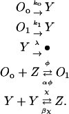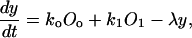
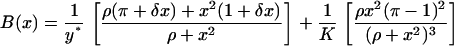
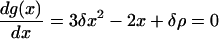
Let O_o, O₁ denote the fraction of free and occupied operator sites, and let y and z be the number of monomer and dimer molecules, respectively. Assuming that the production rates are proportional to the fractions of unoccupied and occupied operator sites and that degradation is a linear function of intracellular content, the single-cell monomer dynamics are described by the equation

(1)

where λ is the degradation rate constant. Due to the conservation of operator sites, we have

(2)

It is further assumed that the occupied and unoccupied states are in equilibrium with each other:

(3)

and that the same holds for the dimerization reaction:

(4)

where α and β are the equilibrium constants of the operator transition and dimerization reactions, respectively. Substituting Eqs. 2–4 into Eq. 1 yields

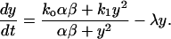(5)

The number of parameters in Eq. 5 can be reduced by nondimensionalizing the intracellular content y and time t as follows:

(6)

(7)

Setting:

(8)

(9)

(10)

(11)

and substituting Eqs. 6–11 into Eq. 5, the following nondimensional form is obtained:

(12)

The reference time t* and reference number of molecules y*, related through Eq. 8, will be fully defined later, when the single-cell model is incorporated into the cell population balance model. We note that since this parameter quantifies the relative magnitude of the rate of monomer production in the unoccupied and occupied states.

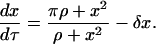
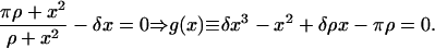
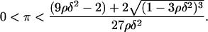
Due to its positive feedback feature, the network dynamics described by Eq. 12 exhibit the classical bistable behavior, where two stable steady states (upper and lower) coexist with an unstable steady state of intermediate magnitude over a significant region of the three-dimensional (π,ρ,δ) parameter space. Since the steady-state version of Eq. 12 has a cubic form, it is possible to analytically find the region of the parameter space where bistability is exhibited. The (π,ρ,δ) bistability region is defined by the following inequalities (see Appendix for proof):

(13)

The model described by Eq. 5 or Eq. 12 is fully deterministic. Hence, it does not account for intrinsic noise at the single-cell level. For this particular genetic network, intracellular noise originates from the small number of molecules as well as from slow operator fluctuations. It is of great interest to understand the implications of these sources of stochasticity on the transient and asymptotic behavior of the system. Since a reaction network is available, such a question can be addressed through Monte Carlo (MC) simulations (33) offering sample paths of the process represented by the master equation formulation (34), and comparison of their predictions with those of Eq. 12. Specifically, by performing multiple MC simulations for each set of parameter values, one can obtain the steady-state marginal density function expressing the probability that the cell has dimensionless intracellular content x.

For single variable systems, stochastic bistability leads to bimodal whereas in regions of the parameter space where the system exhibits only one steady state stochastically, is unimodal (35). By exploring the parameter space this way, one can quantitatively assess the effects of stochasticity at the single-cell level.

For the exploration of the entire parameter space, such simulations can be very time consuming. For this purpose, Kepler and Elston (32) developed a brilliant, Fokker-Planck, fast-and-small noise approximation of the master equation formulation and they applied it to the same genetic network. However, they used a different nondimensionalization with respect to time. To derive the Fokker-Planck approximation that corresponds to the nondimensionalization presented here, we applied their methodology and obtained the following:

(14)

where

(15)

(16)

Equations 14–16 become identical to the corresponding equations presented by Kepler and Elston (32) for δ = 1, a choice that also renders their deterministic single-cell model and ours identical.

One significant advantage of this approximation is that sample paths of the process can be generated in a fraction of the time required for MC simulations, using the stochastic differential equation (SDE) corresponding to the Fokker-Planck Eq. 14 or otherwise known as Langevin equation

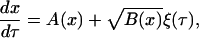(17)

where is a Gaussian white noise process and A(x), B(x) are given by Eqs. 15 and 16, respectively.

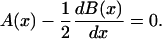
A second advantage is related to the ease by which the effects of stochasticity on the asymptotic single-cell behavior can be computed. The steady-state version of the linear Eq. 14 with reflecting boundary conditions can be easily solved analytically to yield the well-known potential solution (36)

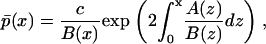(18)

where c is a normalization constant, rendering a density function. Thus, the existence or not of two modes in the shape of the stationary density function can be evaluated for the entire region of the parameter space much quicker than the alternative based on the master equation formulation, which does not allow for analytical solutions. Specifically, the number of modes in can be found by analyzing the solution space of the following, simple algebraic equation

(19)

An additional advantage of this approximation is that it offers analytical insight into the effect of stochasticity on network dynamics. Notice that Eqs. 14 and 17 contain two extra parameters compared to the deterministic single-cell model (Eq. 12): a), the reference number of molecules y*, and b), parameter K, defined as follows:

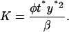(20)

K can be thought as a measure of the rate of operator fluctuations. Thus, the two extra parameters quantify the effect of the two main sources of stochasticity at the single-cell level for the given reaction network, i.e., small numbers of molecules and slow operator fluctuations. We emphasize that there might exist others sources of intrinsic noise in networks with positive feedback architecture, such as bursting, repressor fluctuations, small numbers of mRNA molecules, etc. However, here we consider only those sources of single-cell stochasticity associated only with the given reaction network. Notice also that as (very fast operator fluctuations) and (large numbers of molecules), the Langevin equation (17) becomes identical to the deterministic single-cell model (Eq. 12), since, at these limits, the noise term B(x) vanishes and A(x) yields the right-hand side of Eq. 12.

Comparison between MC simulations and simulations of the Langevin Eq. 17 at various parameter values has shown that the approximation is valid for very small numbers of molecules (y* as low as 25) and very slow operator fluctuations (K as low as 40) as was also shown in the original study. The same also applies when comparing entire steady-state density functions as predicted by the master equation formulation and by the Fokker-Planck approximation. Thus, the latter has a very large range of validity. Based on this result, the analytical expressions (Eqs. 18 and 19) were utilized to assess the effect of the two sources of noise (K and y*) on the region of bistability (i.e., region of the parameter space where is bimodal). Notice (Figs. 1 and 2) that for very fast operator fluctuations and large number of molecules, the regions of stochastic and deterministic bistability overlap, as expected. However, slower operator fluctuations and smaller numbers of molecules have a profound effect on single-cell asymptotic behavior. Small values of K drastically increase the region of bistability. Only for very slow operator fluctuations, a small region of deterministic bistability becomes monostable. Small numbers of molecules have a more pronounced dual effect: they can generate or eliminate bistability although the former effect is visibly more significant. An interesting feature in both cases is the presence of isolated regions of bistability. For example, for fixed values of π, there exist stochastically bistable regions in the ρ parameter space separated by monostable intervals for intermediate values of ρ. This behavior is not exhibited by the corresponding deterministic single-cell model.

FIGURE 1.

Effect of rate of operator fluctuations (K) on the region of bistability at the single-cell level (δ = 1 and y* = 1000). (Solid lines) Single-cell deterministic model (steady state of Eq. 12). (Symbols) Single-cell stochastic model. (a) K = 200,000, (b) K = 2,000, and (c) K = 50.

FIGURE 2.

Effect of number of molecules (y*) on the region of bistability at the single-cell level (δ = 1 and K = 200,000). (Solid lines) Single-cell deterministic model (steady state of Eq. 12). (Symbols) Single-cell stochastic model. (a) y* = 1,000, (b) y* = 50, and (c) y* = 20.

Deterministic cell population balance modeling

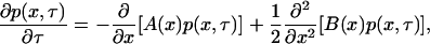
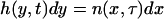
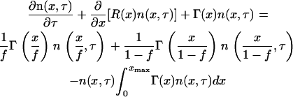
The aforementioned single-cell stochastic model takes into account intrinsic noise, inherently present in regulation of gene expression guided by the function of genetic networks. Thus, it is definitely more realistic than the corresponding deterministic single-cell model. However, by construction, both types of models cannot simulate system behavior at the cell population level. This goal can be achieved with a different class of models, DCPB models first formulated by Fredrickson and co-workers (21–23). The main unknown of a DCPB formulation is the number of cells that at time t have intracellular content between y and y + dy. The generalized DCPB equation for the corresponding number density function h(y,t) in the case of a single intracellular species is as follows (see (31) for a derivation):

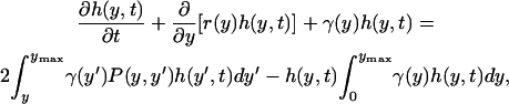(21)

where r(y) is the single-cell reaction rate describing the rate of production or consumption of species y due to intracellular reactions; γ(y) is the single-cell division rate relating cell division with intracellular content; and P(y,y′) is the partition probability density function describing the mechanism by which mother cells of content y′ produce, upon cell division, one daughter cell with content y and another with content y′−y. Assuming no nutrient limitations and in the absence of cell death, these three functions (collectively called intrinsic physiological state functions) fully determine the behavior of the cell population. Finally, y_max is the maximum attainable intracellular content.

The first term of Eq. 21 describes the accumulation of cells with content y, whereas the second term is the rate by which cells with content y are lost from the cell population due to the fact that they react to produce cells of content different than y. The third term accounts for loss of cells with content y due to division yielding daughter cells with smaller content. The first term in the right-hand side describes the birth of new daughter cells of content y from the division of all cells with content greater than y. The factor of 2 accounts for the fact that each division event leads to the birth of two daughter cells. Finally, the second term in the right-hand side describes the dilution effect due to cellular growth. This nonlinear sink term is responsible for the number density function reaching a steady state, known as the state of balanced growth. An appropriate initial condition h_o(y) is used, whereas containment or regularity boundary conditions (23) are used for the solution of Eq. 21, describing the fact that cells of the population do not grow outside the domain [0,y_max]:

(22)

Notice that this model takes into account cell division and explicitly includes the fundamental source of extrinsic population heterogeneity, namely unequal partitioning of mother cell content at cell division. However, this model is fully deterministic despite the presence of a partition probability density function. Therefore, both the single-cell reaction and division rates need to be deterministic functions of intracellular content y. Hence, DCPB models cannot account for stochastic division effects as well as intrinsic noise at the single-cell level, which also constitute important sources of cell population heterogeneity.

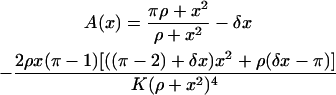
To describe the positive feedback architecture, the single-cell reaction rate describing the rate of change of intracellular content y is taken to be the deterministic single-cell model derived earlier:

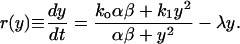(23)

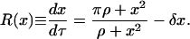
In general, a correlation between the rate by which cells divide and the intracellular content of substances exits even if these substances do not participate in the progression of the cell cycle. To capture such a correlation, a phenomenological power-law expression was used:

(24)

where μ is a measure of the growth rate of the population and has units of inverse time; 〈y〉 represents the average expression level among the cells of the population; and the exponent m quantifies the sharpness of the division rate. This type of functional form for the division rate has also been obtained from experimental data using inverse cell population balance modeling techniques (37).

For the partition probability density function, the simplest possible mechanism describing unequal, asymmetric partitioning at cell division is considered. Specifically, every mother cell is assumed to give a fraction f of its content to one daughter cell and a fraction 1 − f to the other. Clearly, This discrete asymmetric partitioning mechanism is mathematically described by the expression

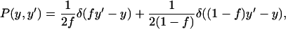(25)

where δ is the delta function. To express Eq. 21 with the nondimensional variables x and τ, Eqs. 6–11 are applied. Moreover, setting

(26)

defining the reference time as

(27)

and substituting the special form of the partition probability density function (Eq. 25) into Eq. 21, the following nonlinear, functional partial differential equation is obtained:

(28)

subject to the boundary conditions

(29)

and an initial condition n_o(x), which is taken to be a truncated Gaussian number density function with mean 〈x〉_o and standard deviation σ_o. The dimensionless single-cell reaction rate R(x) is given by the previously derived, nondimensional, deterministic single-cell model

(30)

Moreover, the nondimensional division rate becomes

(31)

Application of this choice for the reference time t* (Eq. 27) into Eqs. 8, 10, 11, and 20 yields the reference number of molecules and the relationship between all nondimensional and dimensional parameters:

(32)

(33)

(34)

(35)

We note that parameter δ captures the timescale of division relative to protein degradation. In all simulations that will be presented in the following, we used the value of 0.05, which renders protein degradation much slower than division as is the typical case.

The DCPB model defined by Eqs. 28–31 represents a challenging numerical problem. It consists of a nonlinear, functional partial differential equation that has an unknown, upper boundary (x_max). Moreover, due to the nonlinear, single-cell kinetics and the nonlinear term of the equation, it may exhibit multiple steady states of largely different magnitude as is the case with the corresponding single-cell model. These challenges cannot be addressed by standard fixed boundary algorithms. Therefore, a moving boundary algorithm was developed to simulate system behavior both transiently and asymptotically. It consists of an appropriate variable transformation and utilizes a spectral method with sinusoidal basis functions in conjunction with the RK4 time integrator.

Corresponding continuum model

The DCPB model just described predicts the entire distribution of intracellular content and, more importantly, explicitly accounts for the extrinsic sources of cell population heterogeneity. It is of great significance to quantitatively isolate the effects of extrinsic population heterogeneity on system behavior for the given genetic network. However, to achieve such a goal, a corresponding model that also predicts cell population dynamics but neglects cell population heterogeneity is required for comparison purposes. Neglecting cell population heterogeneity implies the assumption that all cells of the population behave the same and exactly like the average cell. Hence, the required model will, by construction, predict only the average population dynamics (since the dynamics of all other cells are identical), and will assume that the cell population is a lumped biophase, behaving like a continuum. For this reason, this type of a model will henceforth be called “continuum model”.

Since the continuum model will only predict the average population dynamics and since it needs to correspond to the DCPB (Eqs. 28–31), the average population dynamics predicted by the DCPB model will need to be derived first. Taking the first moment of Eq. 28, applying the boundary conditions (Eq. 29) as well as conservation of intracellular content at cell division yields

(36)

The assumption that all cells of the population behave exactly like the average cell, which needs to be made for the continuum formulation, is mathematically expressed as follows:

(37)

Substituting Eq. 37 into Eq. 36 yields the continuum model that corresponds to the DCPB model (Eqs. 28–31):

(38)

Thus, comparing the predictions of Eq. 38 with those of the DCPB for the average population behavior will enable the quantitative isolation of the extrinsic population heterogeneity effects. We note that the predictions of Eqs. 36 and 38 will agree only in the special case where the single-cell reaction and division rates are linear functions of the intracellular content, conditions that are certainly not satisfied here.

Figs. 3 and 4 show the effects of the extent of partitioning asymmetry (parameter f) and sharpness of the division rate (parameter m), respectively, on the average, asymptotic expression level. Notice that extrinsic population heterogeneity always shrinks the region of bistability, and at the same time it shifts it toward smaller values of ρ. Moreover, the extent of shrinkage is more pronounced for more asymmetric partitioning and sharper division rates. Very asymmetric partitioning can even eliminate the entire bistability region altogether. In addition, although not directly comparable, it is worth noting that extrinsic heterogeneity affects the asymptotic behavior at the cell population level in the aforementioned, very specific way as opposed to the dual effects that intrinsic noise may have at the single-cell level.

FIGURE 3.

Effect of partitioning asymmetry (f) on average gene expression at the cell-population level as a function of dimensionless parameter ρ (m = 2, π = 0.03, δ = 0.05). (Dashed line) Continuum model. (Solid line, open triangles) f = 0.5. (Dashed line, solid squares) f = 0.4. (Solid line, open squares) f = 0.3. (Dashed line, solid circles) f = 0.2. (Solid line, open circles) f = 0.1.

FIGURE 4.

Effect of sharpness of division rate (m) on average gene expression at the cell-population level as a function of dimensionless parameter ρ (f = 0.3, π = 0.03, δ = 0.05). (Dashed line) Continuum model. (Solid line, open triangles) m = 8.(Dashed line, solid squares) m = 5. (Solid line, open squares) m = 3. (Dashed line, solid circles) m = 2. (Solid line, open circles) m = 1.

From the systems biology perspective, the results in Figs. 3 and 4 establish the critical importance of taking into account cell population heterogeneity to accurately predict system behavior, even if it is of interest to predict only average population property dynamics. Specifically, neglecting extrinsic population heterogeneity may lead to huge differences in the predictions of the qualitative behavior of the system (bistability versus monostability). Furthermore, as shown in Figs. 3 and 4, even in regions of the parameter space where the population is monostable, neglecting population heterogeneity leads to significant overprediction of the average induced state, especially for very asymmetric partitioning and very sharp division rates.

The DCPB model can predict the entire distribution of expression levels. Fig. 5 shows a representative example of the three steady-state number density functions (normalized around the average expression level) coexisting at a given set of parameter values where the cell population exhibits steady-state multiplicity. Notice that the unstable number density function is visibly broader than the two stable ones and that the stable number density function with the lower average is the narrowest of the three, a pattern that persists for other sets of parameter values for which steady-state multiplicity exists.

FIGURE 5.

Three time-invariant number density functions, normalized around the average expression level, coexisting in the bistable regime of the parameter space (m = 2, f = 0.3, π = 0.03, δ = 0.05, and ρ = 0.1). (Solid line, open circles) Stable steady state corresponding to highest average expression level. (Dashed line, solid circles) Unstable steady state corresponding to intermediate average expression level. (Solid line, open squares) Stable steady state corresponding to lowest average expression level.

Fig. 6 shows the normalized steady-state number density function for different extents of partitioning asymmetry in a region of the parameter space where the DCPB exhibits monostable behavior. Notice that more asymmetric partitioning leads to broader number density functions. More importantly, it changes the shape of the number density function from unimodal to bimodal. This is a consequence of the interplay between the particular genetic architecture and the division and partitioning mechanisms. Specifically, due to the autocatalytic nature of the genetic network, the single-cell induction rate has a sigmoidal shape. As a result, there exists a large discrepancy between the induction rates of cells with low and higher expression levels. Thus, cells with low expression levels at a given point in time t require a significantly larger amount of time to become fully induced compared to their peers, which, at the same point in time, have higher expression levels. Higher extent of partitioning asymmetry gives birth to daughter cells that have larger differences in their initial intracellular content. Thus, if the extent of partitioning asymmetry is above a certain threshold (f is below a certain value), the daughter cell with low initial content does not have enough time before division to become fully induced and “catch up” with the daughter cell that was born at the same time but inherited a much larger intracellular content. Hence, if this argument is raised to the entire population level, two distinct subpopulations are formed: one below and one above a certain single-cell induction threshold, thus resulting in the bimodal shape.

FIGURE 6.

Effect of partitioning asymmetry (f) on the shape of the normalized around the average expression level, time-invariant number density function in the monostable regime of the parameter space (m = 2, π = 0.03, δ = 0.05, and ρ = 0.03(Solid line, open circles) f = 0.1. (Dashed line, solid circles) f = 0.2. (Solid line, open squares) f = 0.3. (Dashed line, solid squares) f = 0.4. (Solid line, open triangles) f = 0.5.

Stochastic cell population balance modeling

The DCPB model explicitly accounts for cell division and unequal partitioning of mother cell content and predicts the entire distribution of expression levels instead of just average properties. However, it represents the state of the population at each point in time with a continuous distribution. Hence, it does not “respect” the fact that cells are discrete entities. In addition, the DCPB model is fully deterministic, and thus cannot describe the stochastic nature of cell division, which can in turn significantly influence cell population dynamics in growth stages where cell density is low (24,31). An even more severe consequence of its deterministic nature is that it cannot incorporate intrinsic noise at the single-cell level. Therefore, the DCPB formulation offers only a partial view of cell population heterogeneity and its effects on system behavior. To overcome these shortcomings, a fully discrete and stochastic treatment of cell population dynamics is required. To address this challenge, a fully SVNMC algorithm was developed, the details of the derivation of which are given in Appendix B, whereas a schematic of its basic steps is presented in Fig. 7. The SVNMC model uses the same type of information as the DCPB model (i.e., a single-cell reaction rate, a single-cell division rate, and a partition probability density function) and at the same time accounts for stochastic division, as well as noise associated with intracellular reactions.

FIGURE 7.

Schematic of the SVNMC algorithm that accounts for both intrinsic and extrinsic sources of cell population heterogeneity. See text for detailed description.

To examine the validity of the SVNMC algorithm, consider a hypothetical situation where intrinsic noise has a very small contribution to the expression level dynamics of each individual cell (i.e., and ). Then, the single-cell reaction rate (Eq. 17) would resemble the deterministic single-cell model described by Eq. 12. Moreover, it was shown that for high enough initial cell density and when the single-cell kinetics are fully deterministic, the predictions of the DCPB model are in excellent agreement with those of a VNMC model, which neglects intrinsic noise effects (31). Hence, the predictions of the SVNMC algorithm in cases where intrinsic noise is negligible and the initial cell density is high enough should agree with those of the DCPB model presented earlier. Fig. 8 shows such a comparison for the number density function dynamics. Despite the fact that the two algorithms and mathematical formulations are vastly different, the agreement is excellent. This is true even at early time points where the number density function exhibits abrupt dynamics with complex, multimodal shapes and it also holds throughout the course of the simulation until the cell population reaches a time-invariant state.

FIGURE 8.

Validation of the SVNMC algorithm: comparison of SVNMC predictions (dashed lines) with DCPB model predictions (solid lines) for very low intrinsic noise (K = 50,000, y* = 100,000) and for m = 2, f = 0.2, π = 0.03, δ = 0.05, and ρ = 0.02. (a) τ = 0, (b) τ = 0.195, (c) τ = 0.405, (d) τ = 0.595, (e) τ = 1.005, (f) τ = 1.405, (g) τ = 1.995, (h) τ = 2.995, and (i) τ = 5.

Since the SNVMC algorithm incorporates both intrinsic and extrinsic sources of population heterogeneity in its formulation, whereas the corresponding DCPB model accounts only for extrinsic heterogeneity, comparison of the predictions of the two models can rigorously assess the effects of intrinsic noise on cell population dynamics in regions of the parameter space where intrinsic noise is quantitatively significant. Fig. 9 shows such a comparison. Notice that throughout the course of the simulation and until the population becomes stationary, the multimodal shapes that the number density function obtains deterministically become less well-defined when intrinsic noise is accounted for. Moreover, the population is shifted toward lower average expression levels, whereas the number density function is spread over a wider range of expression levels as also shown in Fig. 10 b. These patterns are general; the results presented in Fig. 9 constitute just a representative example.

FIGURE 9.

Effect of significant intrinsic noise (K = 500, y* = 50) on number density function dynamics for m = 2, f = 0.3, π = 0.03, δ = 0.05, and ρ = 0.07. (Solid lines) Predictions of the DCPB model neglecting intrinsic noise effects. (Dashed lines) Predictions of SVNMC algorithm. (a) τ = 0, (b) τ = 0.2, (c) τ = 0.6, (d) τ = 1, (e) τ = 1.5, (f) τ = 2, (g) τ = 5, (h) τ = 10, and (i) τ = 20.

FIGURE 10.

Decomposing the effects of intrinsic and extrinsic heterogeneity by comparing the predictions of i), the SVNMC model (dashed line), ii), the corresponding DCPB model (solid line), and iii), the corresponding continuum model (solid line, open circles) for the average expression level. Common parameter values in all three models: π = 0.03, δ = 0.05, and ρ = 0.07. Common parameter values for DCPB and SVNMC models: m = 2, f = 0.3. Parameter values appearing only in SVNMC model: K = 500, y* = 50. (a) Average expression levels as predicted by the three models. (b) Coefficients of variation for the number density function as predicted by the SVNMC and DCPB models.

This behavior can be understood when considering the effects that molecular characteristics and division have on the particular genetic architecture. Specifically, low values of y* and K can be due to faster cell division (quantified by μ) relative to the rate of gene expression when the operator is in the occupied state (k₁). In this case, cells produce lower numbers of monomer proteins before cell division occurs. Since cells divide at lower expression levels, the daughter cells will also have lower intracellular content. Thus, the average expression level becomes lower than in the case where intrinsic noise is not considered. Due to the autocatalytic nature of this network, there exists a wide discrepancy in the induction rate between cells with low and high expression levels as is also reflected in the single-cell reaction rate expression (Eq. 12). Thus, the intracellular content of low expressing cells increases much slower than that of cells with expression level above a certain single-cell threshold. Hence, in the case where intrinsic noise is significant and intracellular contents are lower on average, the corresponding number density function is broader as some cells live below and some above the single-cell induction threshold.

Fig. 10 a presents the time evolution of the average expression levels as predicted by the three models starting from the same initial average expression level and the same overall distribution for the DCPB and SVNMC models. Notice that the incorporation of intrinsic noise further amplifies the quantitative effect that extrinsic cell population heterogeneity has on cell population dynamics as the difference between the predictions of the continuum and SVNMC models becomes larger. This further enhances the significance of accounting for population heterogeneity effects, even in cases where predictions of only the average population behavior is of primary interest. Moreover, extrinsic heterogeneity is quantitatively more significant than intrinsic noise, a pattern that persists in other regions of the parameter space as well. Thus, by using these three fundamentally different mathematical formulations, it is possible to obtain deeper insight into the complex relationship between network structure, molecular characteristics of the network, and the distribution of phenotypes among the cells of the entire cell population.

The SVNMC model was subsequently employed to perform bifurcations studies to isolate the intrinsic noise effects on population behavior. For each point in the parameter space, triplicate simulations were performed with the SVNMC algorithm. The population dynamics were simulated for an amount of time sufficient for the main distribution characteristics (average and coefficient of variation) to reach a plateau in the stochastic sense. To capture possible steady-state multiplicity, three different Gaussian initial conditions were used, corresponding to each of the three simulations for every point in the parameter space: a), 〈x〉_o = 0.1, σ_o = 0.025; b), 〈x〉_o = 0.25, σ_o = 0.05; and c), 〈x〉_o = 0.5, σ_o = 0.1.

As expected, for low intrinsic noise levels (high values of K and y*), the asymptotic behavior of the population was found to be practically deterministic since the predictions of the SVNMC model agree with those obtained with the DCPB model and presented in Figs. 3 and 4. However, the situation is different in the presence of significant intrinsic noise. Fig. 11 shows predictions of the SVNMC and DCPB models for the asymptotic behavior of the average expression level as a function of dimensionless parameter ρ for K = 500 and y* = 50. For these parameter values, intrinsic noise has a profound impact on the asymptotic behavior at the single-cell level as was shown in Figs. 1 and 2.

FIGURE 11.

Asymptotic average expression level predicted by the DCPB (solid line) and SVNMC (symbols) models as a function of dimensionless parameter ρ for π = 0.03, δ = 0.05, m = 2, and f = 0.3. Intrinsic noise parameters: K = 500, y* = 50. In the case of SVNMC, the results of three simulations are plotted for each value of ρ.

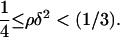
First, notice that in all regions of the parameter space where the system is monostable, both stochastically and deterministically, the population average is always smaller when intrinsic noise is significant. Similar to the special case presented in Fig. 10 b, the corresponding number density function is always broader compared to the deterministic prediction. Second, notice that different, stochastic solutions for the population average exist in the region: This apparent hysteresis in the predictions of the SVNMC model indicates the presence of multiple stationary solutions. As also shown in Fig. 11, multiple steady states coexist deterministically but in a wider region: Therefore, the qualitative effect of intrinsic noise on the bifurcation structure of the system is the same as that of extrinsic heterogeneity: significant intrinsic noise shrinks the region of bistability and shifts it toward lower values of ρ.

This effect of intrinsic noise at the cell population level has fundamental differences from its effect at the single-cell level. As shown in both Figs. 1 and 2, intrinsic noise creates isolated discontinuous bistable regimes in the ρ parameter space for fixed values of π. This is not the case at the cell population level. Moreover, slow operator fluctuations primarily generate very big regions of bistability at the single-cell level (Fig. 1), whereas the effect of noise on the population average is almost the opposite. Although small number of molecules primarily generate bistability, small values of y* can also eliminate significant areas of bistable behavior for high values of ρ. Thus, similar to the observed effect at the population level, small numbers of molecules shift the region of bistability toward lower values of ρ. However, at the cell population level (Fig. 11), this shift is accompanied by a shrinkage of the bistable regime, which is the opposite of what is observed at the single-cell level (Fig. 2).

Fig. 12 illustrates a characteristic example (ρ = 0.1) of bistability loss due to intrinsic noise. The figure shows the time evolution of the average expression level and coefficient of variation of the number density function in the absence and presence of intrinsic noise for two different initial conditions. Notice that in the deterministic case, for low initial averages, the population evolves toward an uninduced state, whereas when the initial average expression is above a certain threshold, the population reaches a different induced state. On the contrary, when intracellular behavior is dominated by noise, the system evolves toward the uninduced state, even for high initial average expression levels, after an initial overshoot in 〈x〉.

FIGURE 12.

Loss of bistability at the population level due to intrinsic noise. Dynamics of average expression level (a) and coefficient of variation of the number density function (b) as predicted by the DCPB (solid lines) and SVNMC (dashed lines) models for two different initial conditions: i), 〈x〉_o = 0.1, σ_o = 0.025; and ii), 〈x〉_o = 0.25, σ_o = 0.05 (open symbols). (a) Average expression level. Parameter values for both models: π = 0.03, δ = 0.05, ρ = 0.1, m = 2, and f = 0.3. Intrinsic noise parameters, K = 500, y* = 50.

DISCUSSION, SUMMARY, AND CONCLUSIONS

The ability to reliably manipulate the genotype of biological organisms offers unique opportunities for understanding, designing, and controlling phenotype. However, biological systems are, within the context of most of their applications, cell populations, and cell populations are heterogeneous systems in the sense that population phenotype is unevenly distributed among the cells of the population. Therefore, to understand and subsequently design and control an organism's phenotype through manipulation of its genotype, we first need to understand the implications of cell population heterogeneity on system behavior. The fundamental biological question under consideration is multi-scale by nature: how do the genetic architecture as well as phenomena and reactions occurring at the single-cell level affect the distribution of phenotypes at the cell population level?

To begin addressing this general, and hence, hard question, we concentrated on a specific network with positive feedback architecture. Cell population heterogeneity originates from two qualitatively different sources: unequal partitioning of cellular material at cell division (extrinsic heterogeneity) and stochastic fluctuations associated with intracellular reactions (intrinsic heterogeneity or intrinsic noise). The primary focus of this work is to quantitatively isolate the effects of these heterogeneity sources on cell population behavior both transiently and asymptotically.

To tackle this problem, we developed a mathematical and computational framework, which consists of the following three modules: a), a continuum model that predicts only the dynamics of the average population behavior and completely neglects population heterogeneity; b), a corresponding DCPB model, which predicts the entire distribution of phenotypes but accounts only for extrinsic population heterogeneity; and c), a corresponding fully stochastic model simulated using a novel SVNMC algorithm, which incorporates all information included in the DCPB model but, in addition, accounts for intrinsic noise at the single-cell level originating from small number of molecules and slow operator fluctuations. Comparison of the predictions of the continuum and DCPB models enables the isolation of extrinsic population heterogeneity effects, whereas comparison of the predictions of the DCPB and SVNMC models allows the isolation of intrinsic noise effects on the behavior of the entire cell population.

The continuum and DCPB models utilize a simple, fully deterministic single-cell model describing the dynamics of the positive feedback loop. On the contrary, the SVNMC algorithm relaxes the deterministic assumption at the single-cell level and utilizes an elegant stochastic, Langevin approximation of the chemical master equation derived by Kepler and Elston (32). The Langevin model collapses to the deterministic single-cell model when intrinsic noise is negligible. Thus, comparison of the predictions of the two models enables the assessment of the effect of intrinsic noise at the single-cell level.

Application of the developed framework illustrates the importance of accounting for population heterogeneity even if prediction of the average population behavior is of primary interest. Furthermore, our results showed that the fundamental sources of extrinsic population heterogeneity, namely, high extent of partitioning asymmetry at cell division as well as sharp division rates, have two key consequences: a), bimodal shapes of the asymptotic number density functions, and b), significant shrinkage of the region of the parameter space where the population exhibits bistable behavior, a characteristic feature of networks with positive feedback architecture. Comparison of the predictions between the DCPB and SVNMC models showed that slow operator fluctuations and small numbers of molecules further shrinks the region of the parameter space where bistability is observed. Moreover, the effect of intrinsic noise at the cell population level was markedly different than at the single-cell level, emphasizing the importance of simulating entire cell populations and not just individual cells to understand the underlying dynamics of a specific genetic network.

Figs. 3, 4, and 11 showed that the different sources of population heterogeneity decrease the bistability region characterizing the asymptotic behavior of cell populations carrying the particular positive feedback loop architecture. From a different perspective, cell population heterogeneity increases the region of the parameter space where the system will evolve toward a unique, monostable number density function irrespective of how far the initial condition is from the asymptotic solution. This might in turn provide insight into how phenotypic variability in systems with positive feedback loops enhances the ability of cell populations to adapt and survive when exposed to severe environmental stresses. Whether the observed trends are specific to this network with the positive feedback architecture or they also apply to other genetic architectures remains a fascinating, open question.

APPENDIX A: REGION OF STEADY-STATE MULTIPLICITY FOR THE DETERMINISTIC, SINGLE-CELL MODEL

The steady-state version of the nondimensional, deterministic single-cell model (Eq. 12) yields the cubic equation

(A1)

From Descartes rule of signs, we can see that Eq. A1 can admit at most three positive real solutions. By setting (s = −x) in Eq. A1 and applying the same rule, we conclude that Eq. A1 can have no negative real solutions. Thus, there exist only two possibilities for the solutions of Eq. A2): a), one positive real and two complex conjugate solutions, and b), three positive real solutions. Here, we are interested in identifying the region of the (π,ρ,δ) parameter space where the latter holds.

Notice that Thus, from Eq. A1, we see that the value of the maximum positive real root can be at most equal to (). Moreover: 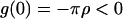and 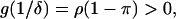since, by definition, Thus, the three positive solutions exist in (). The following two conditions need to be satisfied for three positive real solutions to exist:

• Condition 1 (C1): g(x) must have exactly one maximum x₁ and one minimum x₂ in ().

• Condition 2 (C2): There must exist exactly one solution of Eq. A1 in (x₁,x₂), i.e.,

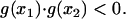
For condition C1 to be satisfied, the equation

(A2)

needs to have exactly two positive solutions. Clearly,

(A3)

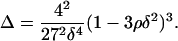
Since and if two real solutions of Eq. A2 exist, then they will definitely be positive. Thus, the condition for existence of two positive real extrema of g(x) reduces to requiring that the discriminant of Eq. A2 is always positive. Therefore, we need to have

(A4)

For condition C2, we first express the product in terms of and and then substitute Eq. A3 to obtain

(A5)

Since for condition C2 to be satisfied, the following inequality needs to hold:

(A6)

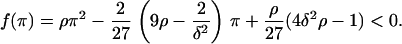
The left-hand side of Eq. A6 is a second order polynomial in π with discriminant

(A7)

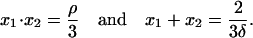
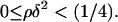
Since Eq. A4 needs to hold, Eq. A7 gives Thus, f(π) will always have two real roots. By taking into account the facts that π > 0 and Eq. A4 needs to hold, we distinguish two cases, for which Eq. A6 is satisfied and hence Eq. A1 has three positive real solutions:

• Case I: f(π) will have a positive and a negative real root and Eq. A6 is satisfied for

  
• Case II: f(π) will have two positive real roots and Eq. A6 is satisfied for

  

APPENDIX B: DERIVATION OF THE SVNMC ALGORITHM

The state (S_τ) of the cell population at a given dimensionless time τ is determined by the total number of cells M_o(τ) and the contents of these cells (X_i(τ)) at time τ. To account for stochasticity, these time-dependent quantities are treated as random variables. Thus

The total number of cells changes as a result of cell division. Given that the population exists at state S_τ at time τ, the time T required for the next division to occur is also a random variable depending on S_τ. To compute T, its cumulative distribution function conditional on S_τ () should be equated to a random number Rand₁ from the uniform distribution. Thus the equation to be solved is

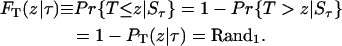(B1)

Since only division disrupts quiescence, the dynamics of the probability that division occurs at T > z given the state of the population S_τ are given by the equation

(B2)

Based on the definition of the initial condition is

(B3)

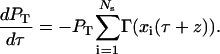
Integrating Eq. B2 subject to Eq. B3 and substituting into Eq. B1 yields the following nonlinear equation for the time between division events T:

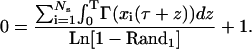(B4)

To compute the integral terms in Eq. B4, one needs to know the intracellular content (expression level) of each individual cell in the population for the time between division events. During this time, all population cells react according to a single-cell reaction rate law R(x). Since we are modeling genetic networks with positive feedback architecture and one of our primary goals is to study the effect of intrinsic noise on cell population dynamics, R(x) will be given by the Langevin Eq. 17 derived earlier, i.e.,

(B5)

where A(x) and B(x) are given by Eqs. 15 and 16, respectively. Thus, Eqs. B4 and B5 are coupled. Hence, to find T, a Newton-Raphson algorithm was used. For the evaluation of the integrals in Eq. B4, the trapezoid rule was implemented (39). To evaluate the intracellular content of each cell at dimensionless time τ + T (required by the trapezoid rule), N_s random numbers ξ_i are chosen from a Gaussian distribution using the joint inversion generating method (40), and the set of SDEs (Eq. B5) are integrated using the one-step, explicit Euler method for SDEs (41). Higher order methods such as the Milstein scheme were also considered. However, the increased computational requirements of such methods rendered them unfavorable to Euler's method. Moreover, more complex quadrature rules than the trapezoid rule were considered for the evaluation of the integrals in Eq. B4. Again, the increased CPU time requirements of such methods were found to be unfavorable compared to the classical and simpler trapezoid rule.

After computing the time between division events, the cell that had undergone division is identified. Defining an indicator variable k such that k = j when a cell with state x_j divides, the conditional distribution function of this random variable, given the state of the entire population at that time, is given by the expression

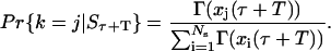(B6)

Thus, by generating another random number from the uniform distribution and finding the corresponding value of j obeying the conditional distribution function (Eq. B6), the cell that had undergone division is identified.

The identification of the mother cell automatically gives its content. Due to the specific choice of the partition probability density function (Eq. 25), the content of the first daughter cell is taken to be the fraction f of the mother cell content. Since mass is conserved at cell division, the content of the other daughter cell is simply obtained by subtracting the content of the first daughter cell from that of the mother cell. Moreover, each division event leads to the “disappearance” of one mother cell and the “appearance” of two newborn cells. Thus, after the determination of the content of each daughter cell, the content of the mother cell is substituted with that of the first daughter cell.

This MC algorithm functions as a hybrid between a constant-volume and a constant-number MC method. Although the sample size is less than a prespecified maximum, it acts as a constant-volume MC with the sample size increasing after each division event and following the dynamics of cell density. However, after the sample size reaches its maximum, it is kept constant for the remainder of the simulation (31). By experimenting with different values of the maximum sample size N_s,max, above which the sample size is kept constant, it was found that for the particular genetic network, 25,000 cells suffice to give accurate simulation results. Therefore, unlike constant-number MC methods, this fully SVNMC algorithm can simulate the process starting from a single cell and until any desirable final time without having the typical CPU time restrictions that constant-volume MC methods have (24,25). Moreover, the ability to simulate very small cell populations allows the assessment of stochastic division effects on cell population dynamics at early growth stages. More importantly, the use of the stochastic single-cell model (Eq. B5) to predict the intracellular dynamics of each cell in the population allows the assessment of single-cell intrinsic noise effects on population-level behavior, as opposed to the simple VNMC algorithm that used a deterministic expression for the single-cell reaction rate (31). In all simulations, a Gaussian distribution was taken as the initial condition using the joint inversion generating method (40).

References

- 1.Delbrück, M. 1945. The burst size distribution in the growth of bacterial viruses (bacteriophages). J. Bacteriol. 50:131–135. [DOI] [PubMed] [Google Scholar]
- 2.Powell, E. O. 1956. Growth rate and generation time of bacteria, with special reference to continuous culture. J. Gen. Microbiol. 15:492–511. [DOI] [PubMed] [Google Scholar]
- 3.Baek, K., S. Svenningsen, H. Eisen, K. Sneppen, and S. Brown. 2003. Single-cell analysis of lambda immunity regulations. J. Mol. Biol. 334:363–372. [DOI] [PubMed] [Google Scholar]
- 4.Ptashne, M. 1987. A Genetic Switch: Gene Control and Phage Lambda. Cell Press, Cambridge, MA, and Blackwell Science, Palo Alto, CA.
- 5.Spudich, J. L., and D. E. Koshland. 1976. Non-genetic individuality: chance in the single cell. Nature. 262:467–476. [DOI] [PubMed] [Google Scholar]
- 6.Stocker, B. A. D. 1949. Measurements of rate of mutation of flagellar antigenic phase in Salmonella typhimurium. J. Hyg. (Camb.). 47:398–413. [DOI] [PMC free article] [PubMed] [Google Scholar]
- 7.Russo-Marie, F., M. Roederer, B. Sager, L. A. Herzenberg, and D. Kaiser. 1993. β-galactosidase activity in single differentiating bacterial cells. Proc. Natl. Acad. Sci. USA. 90:8194–8198. [DOI] [PMC free article] [PubMed] [Google Scholar]
- 8.Chung, J. D., and G. Stephanopoulos. 1995. Studies of transcriptional state heterogeneity in sporulating cultures of Bacillus subtilis. Biotechnol. Bioeng. 47:234–242. [DOI] [PubMed] [Google Scholar]
- 9.Novick, A., and M. Weiner. 1957. Enzyme induction as an all-or-none phenomenon. Proc. Natl. Acad. Sci. USA. 43:553–566. [DOI] [PMC free article] [PubMed] [Google Scholar]
- 10.Maloney, P. C., and B. Rotman. 1973. Distribution of suboptimally induced β-D-galactosidase in Escherichia coli. The enzyme content of individual cells. J. Mol. Biol. 73:77–91. [DOI] [PubMed] [Google Scholar]
- 11.Elowitz, M. B., A. J. Levine, E. D. Siggia, and P. S. Swain. 2002. Stochastic gene expression in a single cell. Science. 297:1183–1186. [DOI] [PubMed] [Google Scholar]
- 12.Block, D. E., P. D. Eitzman, J. D. Wangensteen, and F. Srienc. 1990. Slit scanning of Sacharomyces cerevisiae cells: quantification of asymmetric cell division and cell cycle progression in asynchronous culture. Biotechnol. Prog. 6:504–512. [DOI] [PubMed] [Google Scholar]
- 13.Alberts, B., D. Bray, J. Lewis, M. Raff, M. Roberts, and J. D. Watson. 1994. Molecular Biology of the Cell, 3rd ed. Garland Publishing, New York.
- 14.Volfson, D., J. Marchiniak, W. J. Blake, N. Ostroff, L. S. Tsimring, and J. Hasty. 2006. Origins of extrinsic variability in eukaryotic gene expression. Nature. 439:861–864. [DOI] [PubMed] [Google Scholar]
- 15.Thattai, M., and A. van Oudenaarden. 2001. Intrinsic noise in gene regulatory networks. Proc. Natl. Acad. Sci. USA. 98:8614–8619. [DOI] [PMC free article] [PubMed] [Google Scholar]
- 16.Beckwith, J. R., and D. Zipser, editors. 1970. The Lactose Operon. Cold Spring Harbor Laboratory, Cold Spring Harbor, NY.
- 17.Miller, J. H., and W. S. Reznikoff, editors. 1978. The Operon. Cold Spring Harbor Laboratory, Cold Spring Harbor, NY.
- 18.Ozbudak, E. M., M. Thattai, I. Kurtser, A. D. Grossman, and A. van Oudenaarden. 2002. Regulation of noise in the expression of a single gene. Nat. Genet. 31:69–73. [DOI] [PubMed] [Google Scholar]
- 19.Vilar, J. M. G., C. C. Guet, and S. Leibler. 2003. Modeling network dynamics: the lac operon, a case study. J. Cell Biol. 161:471–476. [DOI] [PMC free article] [PubMed] [Google Scholar]
- 20.Vilar, J. M. G., and S. Leibler. 2003. DNA looping and physical constraints on transcription regulation. J. Mol. Biol. 331:981–989. [DOI] [PubMed] [Google Scholar]
- 21.Eakman, J. M., A. G. Fredrickson, and H. M. Tsuchiya. 1966. Statistics and dynamics of microbial cell populations. Chem. Eng. Prog. 62:37–49. [Google Scholar]
- 22.Tsuchiya, H. M., A.G. Fredrickson, and R. Aris. 1966. Dynamics of Microbial Cell Populations. Adv. Chem. Eng. 6:125–206. [Google Scholar]
- 23.Fredrickson, A. G., D. Ramkrishna, and H. M. Tsuchyia. 1967. Statistics and Dynamics of Prokaryotic Cell Populations. Math. Biosci. 1:327–374. [Google Scholar]
- 24.Shah, B. H., J. D. Borwanker, and D. Ramkrishna. 1976. Monte Carlo simulation of microbial population growth. Math. Biosci. 31:1–23. [Google Scholar]
- 25.Hatzis, C., F. Srienc, and A. G. Fredrickson. 1995. Multistaged corpuscular models of microbial growth: Monte Carlo simulations. Biosystems. 36:19–35. [DOI] [PubMed] [Google Scholar]
- 26.Collins, J. F., and M. H. Richmond. 1962. Rate of growth of Bacillus cereus between divisions. J. Gen. Microbiol. 28:15–33. [DOI] [PubMed] [Google Scholar]
- 27.Collins, J. F., and M. H. Richmond. 1964. The distribution and formation of penicillinase in a bacterial population of Bacillus licheniformis. J. Gen. Microbiol. 34:363–377. [DOI] [PubMed] [Google Scholar]
- 28.Smith, M., and T. Matsoukas. 1998. Constant-number Monte Carlo simulation of population balances. Chem. Eng. Sci. 53:1777–1786. [Google Scholar]
- 29.Lee, K., and T. Matsoukas. 2000. Simultaneous coagulation and break-up using constant-N Monte Carlo. Powder Technol. 110:82–89. [Google Scholar]
- 30.Lin, Y., K. Lee, and T. Matsoukas. 2002. Solution of the population balance equation using constant-number Monte Carlo. Chem. Eng. Sci. 57:2241–2252. [Google Scholar]
- 31.Mantzaris, N. V. 2006. Stochastic and deterministic simulations of cell population dynamics. J. Theor. Biol. 241:690–706. [DOI] [PubMed] [Google Scholar]
- 32.Kepler, T. B., and T. C. Elston. 2001. Stochasticity in transcriptional regulation: origins, consequences, and mathematical representations. Biophys. J. 81:3116–3136. [DOI] [PMC free article] [PubMed] [Google Scholar]
- 33.Gillespie, D. T. 1977. Exact stochastic simulation of coupled chemical reactions. J. Phys. Chem. 81:2340–2361. [Google Scholar]
- 34.Van Kampen, N. G. 1992. Stochastic Processes in Physics and Chemistry. North-Holland, Amsterdam.
- 35.Horsthemke, W., and R. Lefever. 1984. Noise Induced Transitions. Theory and Applications in Physics, Chemistry and Biology. Springer-Verlag, Berlin.
- 36.Gardiner, C. W. 2004. Handbook of Stochastic Methods for Physics, Chemistry and the Natural Sciences. Springer-Verlag, Berlin.
- 37.Dien, B. S. 1994. Aspects of Cell Division Cycle Related Behavior of Saccharomyces cerevisiae Growing in Batch and Continuous Culture: A Single-Cell Growth Analysis. PhD thesis. University of Minnesota, Minneapolis-St. Paul, MN.
- 38.Reference deleted in proof.
- 39.Isaacson, E., and H. B. Keller. 1993. Analysis of Numerical Methods, Dover Publications, New York.
- 40.Gillespie, D. T. 1992. Markov Processes: An Introduction for Physical Scientists. Academic Press, San Diego, CA.
- 41.Kloeden, P. E., and E. Platen. 1999. Numerical Solution of Stochastic Differential Equations. Springer-Verlag. Berlin.