Shrinkage-based similarity metric for cluster analysis of microarray data

Abstract

The current standard correlation coefficient used in the analysis of microarray data was introduced by M. B. Eisen, P. T. Spellman, P. O. Brown, and D. Botstein [(1998) Proc. Natl. Acad. Sci. USA 95, 14863–14868]. Its formulation is rather arbitrary. We give a mathematically rigorous correlation coefficient of two data vectors based on James–Stein shrinkage estimators. We use the assumptions described by Eisen et al., also using the fact that the data can be treated as transformed into normal distributions. While Eisen et al. 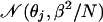use zero as an estimator for the expression vector mean μ, we start with the assumption that for each gene, μ is itself a zero-mean normal random variable [with a priori distribution ], and use Bayesian analysis to obtain a posteriori distribution of μ in terms of the data. The shrunk estimator for μ differs from the mean of the data vectors and ultimately leads to a statistically robust estimator for correlation coefficients. To evaluate the effectiveness of shrinkage, we conducted in silico experiments and also compared similarity metrics on a biological example by using the data set from Eisen et al. For the latter, we classified genes involved in the regulation of yeast cell-cycle functions by computing clusters based on various definitions of correlation coefficients and contrasting them against clusters based on the activators known in the literature. The estimated false positives and false negatives from this study indicate that using the shrinkage metric improves the accuracy of the analysis.

Recent advances in technology, such as microarray-based gene expression analysis, have allowed us to “look inside the cells” by quantifying their transcriptional states. While the most interesting insight can be obtained from transcriptome abundance data within a single cell under different experimental conditions, in the absence of technology to provide one with such a detailed picture, we have to make do with mRNA collected from a small, frequently unsynchronized, population of cells. Furthermore, these mRNAs will give only a partial picture, supported only by those genes that we are already familiar with and possibly missing many crucial undiscovered genes.

Of course, without the proteomic data, transcriptomes tell less than half the story. Nonetheless, it goes without saying that microarrays have already revolutionized our understanding of biology even though they provide only occasional, noisy, unreliable, partial, and occluded snapshots of the transcriptional states of cells.

In an attempt to attain functional understanding of the cell, we try to understand the underlying structure of its transcriptional state-space. Partitioning genes into closely related groups has thus become the key mathematical first step in practically all statistical analyses of microarray data.

Traditionally, algorithms for cluster analysis of genomewide expression data from DNA microarray hybridization are based on statistical properties of gene expressions and result in organizing genes according to similarity in pattern of gene expression. If two genes belong to a cluster then one may infer a common regulatory mechanism for the two genes or interpret this information as an indication of the status of cellular processes. Furthermore, coexpression of genes of known function with novel genes may lead to a discovery process for characterizing unknown or poorly characterized genes. In general, since false negatives (FNs) (where two coexpressed genes are assigned to distinct clusters) may cause the discovery process to ignore useful information for certain novel genes, and false positives (FPs) (where two independent genes are assigned to the same cluster) may result in noise in the information provided to the subsequent algorithms used in analyzing regulatory patterns, it is important that the statistical algorithms for clustering be reasonably robust. Unfortunately, as the microarray experiments that can be carried out in an academic laboratory for a reasonable cost are small in number and suffer from experimental noise, often a statistician must resort to unconventional algorithms to deal with small-sample data.

A popular and one of the earliest clustering algorithms reported in the literature was introduced in ref. 1. In that paper, the gene-expression data are collected on spotted DNA microarrays (2) and based on gene expression in the budding yeast Saccharomyces cerevisiae during the diauxic shift (3), the mitotic cell division cycle (4), sporulation (5), and temperature and reducing shocks. Each entry in a gene expression vector represents a ratio of the amount of transcribed mRNA under a particular condition with respect to its value under normal conditions. All ratio values are log-transformed to treat inductions and repressions of identical magnitude as numerically equal but opposite in sign. It is assumed that the raw ratio values follow log-normal distributions, and hence, the log-transformed data follow normal distributions. Although our mathematical derivations will rely on this assumption for the sake of simplicity, we note that our approach can be generalized in a straightforward manner to deal with other situations where this assumption is violated.

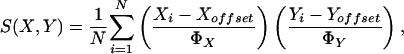
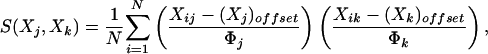
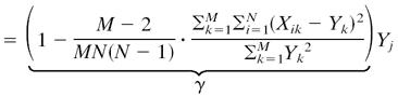
The gene similarity metric used in ref. 1 was a form of correlation coefficient. Let G_i be the (log-transformed) primary data for gene G in condition i. For any two genes X and Y observed over a series of N conditions, the classical similarity score based on Pearson correlation coefficient is:

[1]

where

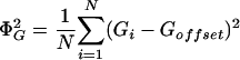[2]

and G_offset is the estimated mean of the observations, i.e.,

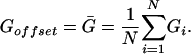Note that Φ_G is simply the (rescaled) estimated standard deviation of the observations. In the analysis presented in ref. 1, “values of G_offset which are not the average over observations on G were used when there was an assumed unchanged or reference state represented by the value of G_offset, against which changes were to be analyzed; in all of the examples presented there, G_offset was set to 0, corresponding to a fluorescence ratio of 1.0.” To distinguish this modified correlation coefficient from the classical Pearson correlation coefficient, we shall refer to it as Eisen correlation coefficient. Our main innovation is in suggesting a different value for G_offset, namely G_offset = γḠ, where γ is allowed to take a value between 0.0 and 1.0. Note that when γ = 1.0, we have the classical Pearson correlation coefficient and when γ = 0.0, we have replaced it by Eisen correlation coefficient. For a nonunit value of γ, the estimator for G_offset = γḠ can be thought of as the unbiased estimator Ḡ being shrunk toward the believed value for G_offset = 0.0. We address the following questions: What is the optimal value for the shrinkage parameter γ from a Bayesian point of view? (See ref. 6 for some alternate approaches.) How do the gene expression data cluster as the correlation coefficient is modified with this optimal shrinkage parameter?

To achieve a consistent comparison, we leave the rest of the algorithms undisturbed. Namely, once the similarity measure has been assumed, we cluster the genes by using the same hierarchical clustering algorithm as the one used by Eisen et al. (1). Their hierarchical clustering algorithm is based on the centroid-linkage method [referred to as the “average-linkage method” of Sokal and Michener (7) in ref. 1] and is discussed further below. The modified algorithm has been implemented by us within the New York University MicroArray Database system and can be freely downloaded from: bioinformatics.cat.nyu.edu/nyumad/clustering/. The clusters created in this manner were used to compare the effects of choosing differing similarity measures.

Model

We derive the proposed similarity metric. In our setup, the microarray data is given in the form of the levels of M genes expressed under N experimental conditions. The data can be viewed as

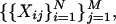where M ≫ N and is the data vector for gene j. We begin by rewriting S (see Eqs. 1 and 2) in our notation:

[3]

In the most general setting, we can make the following assumptions on the data distribution: let all values X_ij for gene j have a normal distribution with mean θ_j and standard deviation β_j (variance β_j²); i.e.,

with j fixed (1 ≤ j ≤ M), where θ_j is an unknown parameter (taking different values for different j). To estimate θ_j, it is convenient to assume that θ_j is itself a random variable taking values close to zero:

The assumed distribution aids us in obtaining the estimate of θ_j given in Eq. 6.

For convenience, let us also assume that the data are range-normalized, so that β_j² = β² for every j. If this assumption does not hold on the given data set, it is easily corrected by scaling each gene vector appropriately. Following common practice, we adjusted the range to scale to an interval of unit length, i.e., its maximum and minimum values differ by 1. Thus,

and

Replacing (X_j)_offset in Eq. 3 by the exact value of the mean θ_j yields a clairvoyant correlation coefficient of X_j and X_k. In reality, since θ_j is itself a random variable, it must be estimated from the data. Therefore, to get an explicit formula for S(X_j, X_k) we must derive estimators for all j.

In Pearson correlation coefficient, θ_j is estimated by the vector mean ; Eisen correlation coefficient corresponds to replacing θ_j by 0 for every j, which is equivalent to assuming (i.e., τ² = 0). We propose to find an estimate of θ_j (call it ) that takes into account both the prior assumption and the data.

First, let us obtain the posterior distribution of θ_j from the prior and the data. This derivation can be done either from the Bayesian considerations or via the James-Stein shrinkage estimators (see refs. 8 and 9). Here, we discuss the former method.

Assume initially that N = 1, i.e., we have one data point for each gene, and denote the variance by σ² for the moment:

From these assumptions, we get (see ref. 10 for full details)

[4]

Now, if N > 1 is arbitrary, X_j becomes a vector X._j. In ref. 10 we show (by using likelihood functions) that the vector of values , with , can be treated as a single data point from the distribution .

Thus, following the same derivation with σ² = β²/N, we have a Bayesian estimator for θ_j given by E(θ_j|X._j):

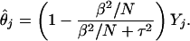[5]

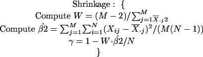
Unfortunately, Eq. 5 cannot be used in Eq. 3 directly, because τ² and β² are unknown, so must be estimated from the data. The details of the estimation are presented in ref. 10.

The resulting explicit estimate for θ_j is

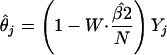[6]

where is an estimator for 1/(β²/N + τ²).

Finally, we substitute from Eq. 6 into the correlation coefficient in Eq. 3 wherever (X_j)_offset appears to obtain an explicit formula for S(X._j, X._k).

Algorithm and Implementation

The implementation of hierarchical clustering proceeds in a greedy manner, always choosing the most similar pair of elements (starting with genes at the bottom-most level) and combining them to create a new element. The “expression vector” for the new element is simply the weighted average of the expression vectors of the two elements that were combined. This structure of repeated pairwise combinations is conveniently represented in a binary tree, whose leaves are the set of genes and internal nodes are the elements constructed from the two children nodes. The algorithm is described below in pseudocode.

Hierarchical clustering pseudocode.

Given

Switch:

Pearson: γ = 1;

Eisen: γ = 0;

While (no. clusters > 1) do

• Compute similarity table:

  
• Find (j*, k*):

  

• Create new cluster N_j*k* = weighted average of G_j* and G_k*.

• Take out clusters j* and k*.

As each internal node can be labeled by a value representing the similarity between its two children nodes, one can create a set of clusters by simply breaking the tree into subtrees by eliminating all the internal nodes with labels below a certain predetermined threshold value.

The implementation of generalized hierarchical clustering with options to choose different similarity measures has been incorporated into the New York University MicroArray Database (NYUMAD), an integrated system to maintain and analyze biological abundance data along with associated experimental conditions and protocols. To enable widespread utility, NYUMAD supports the MAGE-ML standard (www.mged.org/Workgroups/MAGE/mage-ml.html) for the exchange of gene expression data, defined by the Microarray Gene Expression Data Group. More detailed information about NYUMAD can be found at http://bioinformatics.cat.nyu.edu/nyumad/.

Results

Mathematical Simulation. To compare the performance of these algorithms, we started with a relatively simple in silico experiment. In such an experiment, one can create two genes X and Y and simulate N (≈100) experiments as follows:

where α_i, chosen from a uniform distribution over a range [L, H] (), is a “bias term” introducing a correlation (or none if all αs are zero) between X and Y. and are the means of X and Y, respectively. Similarly, σ_X and σ_Y are the standard deviations for X and Y, respectively.

Note that, with this model

if the exact values of the mean and variance are used.

The model was implemented in mathematica (11); the following parameters were used in the simulation: N = 100, τ ∈ {0.1, 10.0} (representing very low or high variability among the genes), σ_X = σ_Y = 10.0, and α = 0 representing no correlation between the genes or representing some correlation between the genes. Once the parameters were fixed for a particular in silico experiment, the gene-expression vectors for X and Y were generated many thousand times, and for each pair of vectors S_c(X, Y), S_p(X, Y), S_e(X, Y), and S_s(X, Y) were estimated by four different algorithms and further examined to see how the estimators of S varied over these trials. These four different algorithms estimated S according to Eqs. 1 and 2 as follows: Clairvoyant estimated S_c by using the true values of θ_X, θ_Y, σ_X, and σ_Y; Pearson estimated S_p by using the unbiased estimators X̄ and Ȳ of θ_X and θ_Y (for X_offset and Y_offset), respectively; Eisen estimated S_e by using the value 0.0 as the estimator of both θ_X and θ_Y; and Shrinkage estimated S_s by using the shrunk biased estimators and of θ_X and θ_Y, respectively. In the latter three, the standard deviation was estimated as in Eq. 2. The histograms corresponding to these in silico experiments can be found in Fig. 1. Our observations are summarized in Table 1.

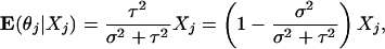
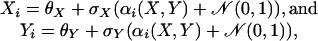
Fig. 1.

Histograms representing the performance of four different estimators of correlation between genes.

Table 1. Summary of observations from mathematical simulation of gene expression models of correlated and uncorrelated genes.

Parameters			Distributions
α	τ		Sc	Sp	Se	Ss
0	0.1	μ	-0.000297	-0.000269	-0.000254	-0.000254
		δ	0.0996	0.0999	0.0994	0.0994
0	10	μ	-0.000971	-0.000939	-0.00119	-0.000939
		δ	0.0994	0.100	0.354	0.100
	0.1	μ	0.331	0.0755	0.248	0.245
		δ	0.132	0.0992	0.0915	0.0915
	10	μ	0.333	0.0762	0.117	0.0762
		δ	0.133	0.100	0.368	0.0999

The distributions of S as estimated by S_c (Clairvoyant), S_p (Pearson), S_e (Eisen), and S_s (Shrinkage) are characterized by the means μ and standard deviations δ. When there is no correlation (α = 0) and low noise (τ = 0.1), all methods do equally well. When there is no correlation but the noise is high (τ = 10), all methods except Eisen do equally well; Eisen has too many FPs. When the genes are correlated and the noise is low, all methods except Pearson do equally well; Pearson has too many FNs. Finally, when the genes are correlated and the noise is high, all methods do equally poorly, introducing FNs; Eisen may also have FPs.

In summary, one can conclude that for the same clustering algorithm, Pearson tends to introduce more FNs and Eisen tends to introduce more FPs than Shrinkage. Shrinkage, on the other hand, reduces these errors by combining the good properties of both algorithms.

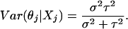
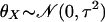
Biological Example. We then proceeded to test the algorithms on a biological example. We chose a biologically well-characterized system and analyzed the clusters of genes involved in yeast cell cycle. These clusters were computed by using the hierarchical clustering algorithm with the underlying similarity measure chosen from the following three: Pearson, Eisen, or Shrinkage. As a reference, the computed clusters were compared to the ones implied by the common cell-cycle functions and regulatory systems inferred from the roles of various transcriptional activators (see Fig. 2).

Fig. 2.

Regulation of cell-cycle functions by the activators. [Reproduced with permission from ref. 12 (Copyright 2001, Elsevier)].

Note that our experimental analysis is based on the assumption that the groupings suggested by the chromatin immunoprecipitation analysis are, in fact, correct and thus, provide a direct approach to compare various correlation coefficients. It is quite likely that the chromatin immunoprecipitation-based groupings themselves contain many false relations (both positive and negative) and corrupt our inference in some unknown manner. Nonetheless, we observe that the trends of reduced false positives and negatives in shrinkage analysis with these biological data are consistent with the analysis based on mathematical simulation and hence, reassuring.

In the work of Simon et al. (12), genomewide location analysis was used to determine how the yeast cell-cycle gene expression program is regulated by each of the nine known cell-cycle transcriptional activators: Ace2, Fkh1, Fkh2, Mbp1, Mcm1, Ndd1, Swi4, Swi5, and Swi6. It was also found that cell-cycle transcriptional activators that function during one stage of the cell cycle regulate transcriptional activators that function during the next stage. This serial regulation of transcriptional activators together with various functional properties suggests a simple way of partitioning some selected cell-cycle genes into nine clusters, each one characterized by a group of transcriptional activators working together and their functions (see Table 2): for instance, group 1 is characterized by the activators Swi4 and Swi6 and the function of budding; group 2 is characterized by the activators Swi6 and Mbp1 and the function involving DNA replication and repair at the juncture of G₁ and S phases, etc.

Table 2. Genes in our data set, grouped by transcriptional activators and cell cycle functions.

Group	Activators	Genes	Functions
1	Swi4, Swi6	Cln1, Cln2, Gic1, Gic2, Msb2, Rsr1, Bud9, Mnn1, Och1, Exg1, Kre6, Cwp1	Budding
2	Swi6, Mbp1	Clb5, Clb6, Rnr1, Rad27, Cdc21, Dun1, Rad51, Cdc45, Mcm2	DNA replication and repair
3	Swi4, Swi6	Htb1, Htb2, Hta1, Hta2, Hta3, Hho1	Chromatin
4	Fkh1	Hhf1, Hht1, Tel2, Arp7	Chromatin
5	Fkh1	Tem1	Mitosis control
6	Ndd1, Fkh2, Mcm1	Clb2, Ace2, Swi5, Cdc20	Mitosis control
7	Ace2, Swi5	Cts1, Egt2	Cytokinesis
8	Mcm1	Mcm3, Mcm6, Cdc6, Cdc46	Prereplication complex formation
9	Mcm1	Ste2, Far1	Mating

Upon closer examination of the data, we observed that the data in its raw “prenormalized” form is inconsistent with the assumptions used in deriving γ: (i) the gene vectors are not range-normalized, so β_j² ≠ β² for every j, and (ii) the N experiments are not necessarily independent.

Range normalization and subsampling of experiments were used before clustering in an attempt to alleviate these shortcomings. The clusters on the processed data set, thresholded at the cut-off value of 0.60, are listed in Tables 3, 4, 5. The choice of the threshold parameter is discussed further in Discussion.

Table 3. Range-normalized subsampled data, γ = 0.0 (Eisen).

Clusters	Activators	Genes
E58	Swi4/Swi6	Cln1, Och1
E68	Swi4/Swi6	Cln2, Msb2, Rsr1, Bud9, Mnn1, Exg1
	Swi6/Mbp1	Rnr1, Rad27, Cdc21, Dun1, Rad51, Cdc45, Mcm2
	Swi4/Swi6	Htb1, Htb2, Hta1, Hta2, Hho1
	Fkh1	Hhf1, Hht1, Arp7
	Fkh1	Tem1
	Ndd1/Fkh2/Mcm1	Clb2, Ace2, Swi5
	Ace2/Swi5	Egt2
	Mcm1	Mcm3, Mcm6, Cdc6
E29	Swi4/Swi6	Gic1
E64	Swi4/Swi6	Gic2
E33	Swi4/Swi6	Kre6, Cwp1
	Swi6/Mbp1	Clb5, Clb6
	Swi4/Swi6	Hta3
	Ndd1/Fkh2/Mcm1	Cdc20
	Mcm1	Cdc46
E73	Fkh1	Tel2
E23	Ace2/Swi5	Cts1
E43	Mcm1	Ste2
E66	Mcm1	Far1

Table 4. Range-normalized subsampled data, γ = 0.66 (Shrinkage).

Clusters	Activators	Genes
S49	Swi4/Swi6	Cln1, Bud9, Och1
	Ace2/Swi5	Egt2
	Mcm1	Cdc6
S6	Swi4/Swi6	Cln2, Gic2, Msb2, Rsr1, Mnn1, Exg1
	Swi6/Mbp1	Rnr1, Rad27, Cdc21, Dun1, Rad51, Cdc45
S32	Swi4/Swi6	Gic1
S65	Swi4/Swi6	Kre6, Cwp1
	Swi6/Mbp1	Clb5, Clb6
	Fkh1	Tel2
	Ndd1/Fkh2/Mcm1	Cdc20
	Mcm1	Cdc46
S15	Swi6/Mbp1	Mcm2
	Mcm1	Mcm3
S11	Swi4/Swi6	Htb1, Htb2, Hta1, Hta2, Hho1
	Fkh1	Hhf1, Hht1
S60	Swi4/Swi6	Hta3
S30	Fkh1	Arp7
	Ndd1/Fkh2/Mcm1	Clb2, Ace2, Swi5
S62	Fkh1	Tem1
S53	Ace2/Swi5	Cts1
S14	Mcm1	Mcm6
S35	Mcm1	Ste2
S36	Mcm1	Far1

Table 5. Range-normalized subsampled data, γ = 1.0 (Pearson).

Clusters	Activators	Genes
P1	Swi4/Swi6	Cln1, Och1
P15	Swi4/Swi6	Cln2, Rsr1, Mnn1
	Swi6/Mbp1	Cdc21, Dun1, Rad51, Cdc45, Mcm2
	Mcm1	Mcm3
P29	Swi4/Swi6	Gic1
P2	Swi4/Swi6	Gic2
P3	Swi4/Swi6	Msb2, Exg1
	Swi6/Mbp1	Rnr1
P51	Swi4/Swi6	Bud9
	Ndd1/Fkh2/Mcm1	Clb2, Ace2, Swi5
	Ace2/Swi5	Egt2
	Mcm1	Cdc6
P11	Swi4/Swi6	Kre6
P62	Swi4/Swi6	Cwp1
	Swi6/Mbp1	Clb5, Clb6
	Swi4/Swi6	Hta3
	Ndd1/Fkh2/Mcm1	Cdc20
	Mcm1	Cdc46
P49	Swi6/Mbp1	Rad27
	Swi4/Swi6	Htb1, Htb2, Hta1, Hta2, Hho1
	Fkh1	Hhf1, Hht1
P10	Fkh1	Tel2
	Mcm1	Mcm6
P23	Fkh1	Arp7
P50	Fkh1	Tem1
P69	Ace2/Swi5	Cts1
P42	Mcm1	Ste2
P13	Mcm1	Far1

Our initial hypothesis can be summarized as follows: Genes expressed during the same cell-cycle stage and regulated by the same transcriptional activators should be in the same cluster. We compared the performance of the similarity metrics based on the degree to which each of them deviated from this hypothesis. Below we list some of the observed deviations from the hypothesis.

Possible FPs.

• Bud9 (group 1: budding), Egt2 (group 7: cytokinesis), and Cdc6 (group 8: prereplication complex formation) are placed in the same cluster by all three metrics: (E68, S49, and P51).

• Mcm2 (group 2: DNA replication and repair) and Mcm3 (group 8) are placed in the same cluster by all three metrics: (E68, S15, and P15).

• For more examples, see ref. 10.

Possible FNs. Group 1: budding (Table 2) is split into five clusters by the Eisen metric: {Cln1, Och1} ∈ E58, {Cln2, Msb2, Rsr1, Bud9, Mnn1, Exg1} ∈ E68, Gic1 ∈ E29, Gic2 ∈ E64, and {Kre6, Cwp1} ∈ E33; into four clusters by the Shrinkage metric: {Cln1, Bud9, Och1} ∈ S49, {Cln2, Gic2, Msb2, Rsr1, Mnn1, Exg1} ∈ S6, Gic1 ∈ S32, and {Kre6, Cwp1} ∈ S65; and into eight clusters by the Pearson metric: {Cln1, Och1} ∈ P1, {Cln2, Rsr1, Mnn1} ∈ P15, Gic1 ∈ P29, Gic2 ∈ P2, {Msb2, Exg1} ∈ P3, Bud9 ∈ P51, Kre6 ∈ P11, and Cwp1 ∈ P62.

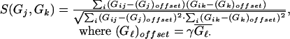
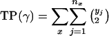
We introduced a new notation to represent the resulting cluster sets, and a scoring function to aid in their comparison.

Each cluster set can be written as follows:

where x denotes the group number (as described in Table 2), n_x is the number of clusters group x appears in, and for each cluster j ∈ {1,..., n_x} there are y_j genes from group x and z_j genes from other groups in Table 2. A value of * for z_j denotes that cluster j contains additional genes, although none of them are cell-cycle genes. The cluster set can then be scored according to the following measure:

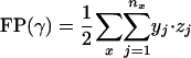[7]

[8]

[9]

Table 2 contains those genes from Fig. 2 that were present in our data set. Tables 3, 4, 5 contain these genes grouped into clusters by a hierarchical clustering algorithm using the three metrics (Eisen in Table 3, Shrinkage in Table 4, and Pearson in Table 5) thresholded at a correlation coefficient value of 0.60. Genes that have not been grouped with any others at a similarity of 0.60 or higher are absent from the tables; in the subsequent analysis they are treated as singleton clusters.

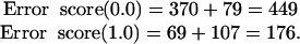
The subsampled data yielded the estimate γ ≃ 0.66. In our set notation, the resulting Shrinkage clusters with the corresponding error score computed as in Eq. 9 can be written as follows:

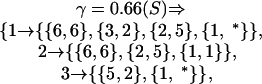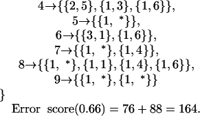The error scores for the Eisen (γ = 0.0) and Pearson (γ = 1.0) cluster sets, computed according to Eq. 9, are

From the data shown in Tables 3, 4, 5, as well as by comparing the error scores, one can conclude that for the same clustering algorithm and threshold value, Pearson tends to introduce more FNs and Eisen tends to introduce more FPs than Shrinkage, as Shrinkage reduces these errors by combining the good properties of both algorithms. This observation is consistent with our mathematical analysis and the simulation presented above.

We have also conducted a more extensive computational analysis of Eisen's data, but omitted it from this article because of space limitations. This analysis appears in a full technical report available for download from www.cs.nyu.edu/cs/faculty/mishra/ (10).

Discussion

Microarray-based genomic analysis and other similar high-throughput methods have begun to occupy an increasingly important role in biology, as they have helped to create a visual image of the state-space trajectories at the core of cellular processes. This analysis will address directly to the observational nature of the new biology. As a result, we need to develop our ability to “see,” accurately and reproducibly, the information in the massive amount of quantitative measurements produced by these approaches or be able to ascertain when what we see is unreliable and forms a poor basis for proposing novel hypotheses. Our investigation demonstrates the fragility of many of these analysis algorithms when used in the context of a small number of experiments. In particular, we see that a small perturbation of, or a small error in the estimation of, a parameter (the shrinkage parameter) has a significant effect on the overall conclusion. The errors in the estimators manifest themselves by missing certain biological relations between two genes (FNs) or by proposing phantom relations between two otherwise unrelated genes (FPs).

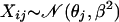
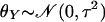
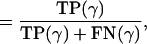
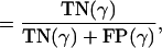
A global picture of these interactions can be seen in Fig. 3, the receiver operator characteristic (ROC) figure, with each curve parametrized by the cut-off threshold in the range of [–1, 1]. An ROC curve (13) for a given metric plots sensitivity against (1–specificity), where

Fig. 3.

Receiver operator characteristic curves. Each curve is parametrized by the cut-off value θ ∈ {1.0, 0.95,..., –1.0}.

Sensitivity = fraction of positives detected by a metric

[10]

Specificity = fraction of negatives detected by a metric

[11]

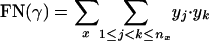
and TP(γ), FN(γ), FP(γ), and TN(γ) denote the number of true positives, false negatives, false positives, and true negatives, respectively, arising from a metric associated with a given γ. (Recall that γ is 0.0 for Eisen, 1.0 for Pearson, and is computed according to Eq. 6 for Shrinkage, which yields 0.66 on this data set.) For each pair of genes, {j, k}, we define these events using our hypothesis (see above) as a measure of truth:

TP: {j, k} are in the same group (see Table 2) and {j, k} are placed in the same cluster;

FP: {j, k} are in different groups, but {j, k} are placed in the same cluster;

TN: {j, k} are in different groups and {j, k} are placed in different clusters; and

FN: {j, k} are in the same group, but {j, k} are placed in different clusters.

FP(γ) and FN(γ) were already defined in Eqs. 7 and 8, respectively, and we define

[12]

and

[13]

where Total = = 946 is the total no. of gene pairs {j, k} in Table 2.

Fig. 3 suggests the best threshold to use for each metric and can also be used to select the best metric to use for a particular sensitivity.

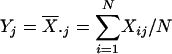
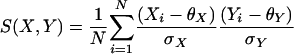
The dependence of the error scores on the threshold can be more clearly seen from Fig. 4. It shows that the conclusions we draw above hold for a wide range of threshold values, and hence a threshold value of 0.60 is a reasonable representative value.

Fig. 4.

FN and FP curves, plotted as functions of θ.

As a result, to study the clustering algorithms and their effectiveness, one may ask the following questions. If one must err, is it better to err on the side of more FPs or more FNs? What are the relative costs of these two kinds of errors? Intelligent answers to our questions depend crucially on how the cluster information is used in the subsequent discovery processes.

References

- 1.Eisen, M. B., Spellman, P. T., Brown, P. O. & Botstein, D. (1998) Proc. Natl. Acad. Sci. USA 95, 14863–14868. [DOI] [PMC free article] [PubMed] [Google Scholar]
- 2.Schena, M., Shalon, D., Heller, R., Chai, A., Brown, P. O. & Davis, R. W. (1996) Proc. Natl. Acad. Sci. USA 93, 10614–10619. [DOI] [PMC free article] [PubMed] [Google Scholar]
- 3.DeRisi, J. L., Iyer, V. R. & Brown, P. O. (1997) Science 278, 680–686. [DOI] [PubMed] [Google Scholar]
- 4.Spellman, P. T., Sherlock, G., Zhang, M., Iyer, V. R., Anders, K., Eisen, M. B., Brown, P. O., Botstein, D. & Futcher, B. (1998) Mol. Biol. Cell 9, 3273–3297. [DOI] [PMC free article] [PubMed] [Google Scholar]
- 5.Chu, S., DeRisi, J. L., Eisen, M. B., Mulholland, J., Botstein, D., Brown, P. O. & Herskowitz, I. (1998) Science 282, 699–705. [DOI] [PubMed] [Google Scholar]
- 6.MacKay, D. J. C. (1992) Neural Comput. 4, 415–447. [Google Scholar]
- 7.Sokal, R. R. & Michener, C. D. (1958) Univ. Kans. Sci. Bull. 38, 1409–1438. [Google Scholar]
- 8.James, W. & Stein, C. (1961) in Proceedings of the Fourth Berkeley Symposium on Mathematical Statistics, ed. Neyman, J. (Univ. of California Press, Berkeley), Vol. 1, pp. 361–379. [Google Scholar]
- 9.Hoffman, K. (2000) Stat. Pap. 41, 127–158. [Google Scholar]
- 10.Cherepinsky, V., Feng, J., Rejali, M. & Mishra, B. (2003) NYU CS Technical Report 2003-845 (New York University, New York).
- 11.Wolfram, S. (1999) The Mathematica Book (Cambridge University Press, Cambridge, U.K.), 4th Ed.
- 12.Simon, I., Barnett, J., Hannett, N., Harbison, C. T., Rinaldi, N. J., Volkert, T. L., Wyrick, J. J., Zeitlinger, J., Gifford, D. K., Jaakkola, T. S. & Young, R. A. (2001) Cell 106, 697–708. [DOI] [PubMed] [Google Scholar]
- 13.Egan, J. P. (1975) Signal Detection Theory and ROC Analysis (Academic, New York).