Minimal haplotype tagging

Abstract

The high frequency of single-nucleotide polymorphisms (SNPs) in the human genome presents an unparalleled opportunity to track down the genetic basis of common diseases. At the same time, the sheer number of SNPs also makes unfeasible genomewide disease association studies. The haplotypic nature of the human genome, however, lends itself to the selection of a parsimonious set of SNPs, called haplotype tagging SNPs (htSNPs), able to distinguish the haplotypic variations in a population. Current approaches rely on statistical analysis of transmission rates to identify htSNPs. In contrast to these approximate methods, this contribution describes an exact, analytical, and lossless method, called BEST (Best Enumeration of SNP Tags), able to identify the minimum set of SNPs tagging an arbitrary set of haplotypes from either pedigree or independent samples. Our results confirm that a small proportion of SNPs is sufficient to capture the haplotypic variations in a population and that this proportion decreases exponentially as the haplotype length increases. We used BEST to tag the haplotypes of 105 genes in an African-American and a European-American sample. An interesting finding of this analysis is that the vast majority (95%) of the htSNPs in the European-American sample is a subset of the htSNPs of the African-American sample. This result seems to provide further evidence that a severe bottleneck occurred during the founding of Europe and the conjectured “Out of Africa” event.

Single-nucleotide polymorphisms (SNPs) are an invaluable tool to uncover the genetic basis of common diseases (1, 2) by providing a high-resolution map of the genome and allowing researchers to associate variations in a particular genomic region to observable traits. Unfortunately, the sheer number of SNPs in the human genome, which makes SNPs so useful as markers, also makes genomewide association studies unfeasible. However, the number of distinct combinations of SNP alleles (haplotypes) encountered in human samples is a small fraction of the possible haplotypes that would arise if alleles were distributed randomly. This haplotypic structure of the genome lends itself to the selection of a parsimonious set of SNPs, called haplotype tagging SNPs (htSNPs), able to distinguish the haplotypic variations in a population.

Given a set of haplotypes in a genomic region, identified through statistical (3, 4) or molecular (5, 6) methods, the process of haplotype tagging is in principle deterministic. Unfortunately, this problem is also computationally intractable (7), because its solution requires the testing of every possible combination of SNPs in the haplotype set, and the number of these combinations grows exponentially with the number of SNPs in the haplotype set. Current approaches rely on approximate methods to identify htSNPs. Most efforts (8–12) have focused on the identification of a secondary haplotype structure across several large regions of the genome. This substructure comprises regions of limited recombination, called haplotype blocks, bounded by small regions characterized by higher recombination rates. Within these smaller regions, htSNPs can be readily identified by eye or by brute-force search. An alternative approach (13) searches for htSNPs by maximizing the haplotype diversity “explained” by a set of SNPs. Using this method, Johnson et al. (13) were able to identify htSNPs accounting for up to 80% of the genomic variations in the populations they analyzed. Despite their differences, both block-based and direct approaches use stochastic methods to identify a reduced set of SNPs sufficient to characterize a genomic region in a population. A common concern about these approaches is that the loss of information induced by their stochastic nature could lead to overlooking rare variations responsible for less frequent diseases (14).

In contrast to these approximate approaches, we introduce the first exact, analytical, lossless solution to the problem of identifying the minimum set of SNPs accounting for the variations in an arbitrary genomic region. This method, called Best Enumeration of SNP Tags (BEST), does not follow a suboptimal heuristic or some approximate, stochastic approach but takes advantage of a peculiar aspect of the genome (the relatively small number of haplotypes with respect to the number of SNPs) to confine the source of complexity to a smaller search space. In this way, the reliability of the identified htSNPs will be only a function of the inferred haplotypes, and the haplotype tagging process will not induce any further information loss. Experimental results show that BEST runs to completion in a matter of seconds even for genomic regions containing >200 SNPs.

The method described in this contribution can take as input haplotypes inferred from cross-sectional samples via stochastic systems (3, 4) or from pedigree data. Therefore, we applied our method to both a set of 105 genes from 47 independent subjects and haplotypes for 9 genes from pedigree data described in ref. 13. Our results confirm that a small proportion of SNPs is sufficient to capture the haplotypic variations in a population and show that this proportion decreases exponentially as the number of SNPs in the haplotype increases. Comparing BEST to the method proposed by Johnson et al. (13), we also show that, in two genes of nine, our method finds smaller sets of htSNPs, suggesting that BEST improves their original results, even for comparatively small haplotypes.

Materials

Data Collection. SNP genotype data for 24 self-described African Americans (12 female) and 23 European Americans (11 female) were obtained for 105 genes: 85 genes from the University of Washington–Fred Hutchinson Cancer Research Center Variation Discovery Resource Program for Genomic Applications (http://pga.mbt.washington.edu) and 20 genes from the Innate Immunity Programs for Genomic Applications (http://innateimmunity.net). All sequencing was performed on the same anonymized DNA samples from the Coriell Cell Repositories (http://locus.umdnj.edu/nigms), using the same Big Dye Terminator sequencing chemistry and equipment (Applied Biosystems). Both sites used the same software and virtually identical protocols for base calling, assembly, and SNP determination, as detailed on each of the respective web sites.

We also tested our method by using published haplotypes, which included 5 genes in a maximum of 418 multiplex families from the Diabetes UK Warren 1 Repository, 3 genes in 598 subjects from Finnish families with at least one sibling diagnosed with type 1 diabetes, and one gene from United Kingdom blood donors (13).

Haplotype Identification. Haplotypes comprising all SNPs with minor allele frequency of ≥10% were inferred for each gene, independently in each ethnic sample, by using default settings of the phase program (3) for each of the 105 genes. To account for the inherent error rate of current genotyping technologies, we selected only those haplotypes seen more than once (frequency of >4%).

Methods

Preliminary Definitions. We regard a SNP as a variable bearing, at most, four states, one for each of the possible alleles (A, T, G, and C), although, in practice, SNPs with more than two states are relatively uncommon. This variable can also encode insertion (+) and deletion (–) polymorphisms. An allele is the assignment of a value to a SNP: we will say that, in a particular individual, the SNP in a particular locus bears the value. A haplotype is a set of contiguous alleles, as they appear in the population of interest. A haplotype set is a set of contiguous SNPs, and it is identified by a set of haplotypes found in the population of interest. Fig. 1 shows the unique haplotypes from SNPs with ≥10% rare allele frequency found in gene TLR7 from an African-American sample; columns represent SNPs, rows represent haplotypes, cells represent alleles, and the entire table is the haplotype set.

Fig. 1.

The haplotype set of gene TLR7 in an African-American sample. Each column represents a SNP, and each row represents a haplotype identified in the sample. In this case, there are 14 haplotypes spanning 59 SNPs. Color coding for each SNP is performed by selecting the first (in this case, the most frequent) haplotype and coloring alleles with the same value as the first haplotype in red. The alternative allele is colored blue. The first row of labels assigns a number to each SNP, and the second row of labels specifies whether the SNP is a htSNP (no label), a derivable SNP (marked by X), or a binary equivalent SNP (labeled with its first binary equivalent in the haplotype set). For example, the first SNP is derivable, the second SNP is binary equivalent to 1, and the third SNP is a htSNP. The last column reports the frequency of each haplotype in the sample.

A haplotype set can be a haplotype block, an entire gene, or an arbitrary genomic region. A SNP is derivable from a set of SNPs if its alleles are uniquely identified by a combination of alleles of the SNPs in such a set. A set of SNPs is sufficient to derive the SNPs in a haplotype set if all the SNPs in the haplotype set can be derived from the SNPs in such set. A set of SNPs is necessary to derive the SNPs in a haplotype set if, when one of its members is removed, at least one SNP in the haplotype set, including itself, is no longer derivable. A tagging set is the set of SNPs in a haplotype set necessary and sufficient to derive all of the SNPs in the set. Among all of the tagging sets, a minimal tagging set is a set containing the minimum number of SNPs, and its members will be called htSNPs. For a given haplotype set, there may be more than one minimal tagging set. Our goal is to find at least one of them.

Haplotype Tagging. Fig. 2 gives a skeletal description of the haplotype tagging algorithm BEST. The algorithm takes as input a set S of haplotypes, each representing a unique set of values of each SNP in the haplotype set, such as the haplotype set displayed in Fig. 1. The algorithm returns a minimal set of SNPs from which all of the other SNPs in the haplotype set can be derived. A preliminary step of the algorithm is to convert the haplotype set into binary form. The colors in Fig. 1 encode the binary conversion of a haplotype set. Although we consider here only the case of biallelic SNPs, this encoding can be easily generalized to triallelic SNPs and is currently implemented as such. When two SNPs share the same binary representation, they are termed binary equivalent. Any tagging set including a SNP will be equivalent to a tagging set where it is replaced by one of its binary equivalent SNPs. After the binary conversion, the algorithm will keep only one member of each group of binary equivalent SNPs.

Fig. 2.

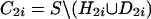
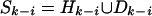
Skeletal description of the BEST algorithm. A lowercase letter denotes a SNP, an uppercase letter denotes a set of SNPs, and a calligraphic uppercase letter denotes a set of sets. The symbol \ denotes the set-theoretic operation of subtraction, |Y| denotes the number of elements in the set Y, h denotes a tagging SNP, denotes a tagging set, denotes a set of alternative tagging sets, c denotes a SNP not included in a tagging set, C denotes the set of such SNPs, and * and ** are auxiliary variables storing alternative tagging sets. The function DERIVED(Y) returns the SNP set derivable from the SNP set Y, and DERIVABLE(x,Y) is true if the SNP x is derivable from the SNP set Y.

A fundamental property of this binary representation is that if a SNP is derivable from a set of other SNPs, then it will be derivable from any superset of such a set. This property spares the exponential effort of identifying the set of SNPs deriving a SNP. The second critical property exploited by BEST is that the tagging set identified by adding, at each step, the SNP that derives the maximum number of SNPs leads to SNP sets containing the minimal tagging set.

Let S = {s₁,..., s_m} denote the m SNPs in a haplotype set. BEST recursively partitions the set S in two groups H and D such that S = H – D, where H is the minimal tagging set (the smallest set of SNPs necessary and sufficient to derive all of the SNPs in the haplotype set), D is the set of (m – k) SNPs that are derivable from H, and a SNP d_j is derivable from H if the value of d_j in each haplotype can be expressed as a Boolean function f(.) of elements of H. A property of these Boolean functions is that if a SNP d_j is derivable from a subset H′ of H, then d_j is also derivable from any subset of H containing H′. This property follows from the fact that if a SNP is derivable from set of SNPs H′, then its alleles are uniquely identified by the allele combinations of the SNPs in H. Therefore, f(h₁,..., h_k) = f(h₁,..., h_k, h_k+1, h_k+2,...) for all h₁,..., h_k in H′. In this way, one can check whether a SNP s_j is derivable from a subset of SNPs in S without necessarily knowing the specific subset, therefore avoiding the exponential cost of the search. In the skeletal description of the algorithm in Fig. 2, this operation is performed by the function DERIVABLE(x, Y), which returns true if the combinations of the alleles of a subset of the SNPs in the set Y uniquely identify the alleles of the SNP x. The function DERIVED(Y) returns the set of SNPs derivable from the set of SNPs Y. We can show that the cost of the function DERIVED(Y) is polynomial by noting that if a SNP x is derivable from a set of SNPs Y, it is also derivable by any superset of Y. Hence, to check the derivability of a SNP x from a set Y, we just check whether the alleles of at least one member of Y match the alleles of x. The function DERIVED(Y) is a simple iteration of the function DERIVABLE(x,Y) across the SNP set Y and can be executed in polynomial time.

The first step of the algorithm is the generation of the set H₁ of htSNPs that are not derivable from any subset of S. This set is identified by examining the Boolean dependency of each s_j on the set of SNPs S \ s_j, and each s_j that is not derivable is assigned to H₁. The elements of H₁ determine a partition of the remaining SNPs into . The set D₁ contains the SNPs derivable from H₁, whereas C₁ is the set of SNPs that are not derivable from H₁ and are therefore candidate htSNPs. Next, an augmentation procedure is applied to move one or more elements from C₁ to H₁ and from C₁ to D₁. First, the elements of C₁ are sorted according to this criterion: if the set D_2i of SNPs derivable from has cardinality greater than the cardinality of the set D_2j of SNPs derivable from . If the criterion identifies only one c₁ such that for all other c_j in C₁, then , D₂ = D₂₁, and , and the procedure is repeated on the set C₂ until the set of candidate SNPs is empty. When more than one set D_2i of SNPs derivable from has the same size of D₂₁, then parallel partitions , D_2i and D_2i) are generated, and the augmentation procedure is repeated on each of them. When none of the SNPs in C₁ augments the set D₁, then pairs of SNPs are treated as one single variable by the augmentation procedure. When the set of candidate SNPs is empty, if the augmentation procedure returns one or more necessary and sufficient sets H of htSNPs, then the algorithm stops. If no such set is found, the whole procedure is repeated on each of the sets H.

Proof of Optimality. We prove by induction on k, the minimum number of htSNPs, that the smallest set of necessary and sufficient htSNPs returned by BEST is the minimum set of htSNPs tagging the haplotype set at hand. Suppose first that k = 1, so that the minimum set of htSNPs consists only of one SNP. Because k = 1, then all elements of S are binary equivalent and BEST will return one of the m minimal tagging sets, each set given by {s_i}, for i = 1,..., m. Any of this set will be the minimum solution. Next, suppose the result is true for any minimum set of size k – 1 (that is, if the minimum set of htSNPs has size j ≤ k – 1, then we assume that BEST returns one of the minimum solutions of size j) and we show that the result is true when the minimum set consists of k htSNPs. More precisely, we assume that H = {h₁,..., h_n} is the set returned by BEST ordered according to the augmentation procedure, and we show that n = k. Suppose that we can decompose the set of SNPs S into , where S_k–1 is the subset of S that is decomposed into , D_k–1, H_k–1 consists of the first k – 1 htSNPs in H, D_k–1 is the set of SNPs that are derivable from H_k–1, and S_k is the set of SNPs in S that are not derivable from H_k–1. By induction, H_k–1 is the minimum set of htSNPs for S_k–1, and it is equivalent to any minimum set of htSNPs for S_k–1. Furthermore, because we are assuming there is a minimum solution of size k, there exists at least one htSNP in S_k that, once added to H_k–1, makes of the minimum set of htSNPs. Because the set of SNPs derivable from is the whole set , then the cardinality of the set of SNPs derivable from is the largest, and therefore is the set of htSNPs found by BEST and n = k. If a decomposition does not exist, then we can decompose , where and H_k–i consists of the first (k – i) SNPs, and repeat the same argument.

Results

BEST was first used to tag the 105 genes, ranging from 5 to 229 SNPs in length, described in Materials. The results of this analysis are summarized in Table 1. These results confirm that a small proportion of SNPs (14% for African Americans and 10% for European Americans) is sufficient to capture the variations in a haplotype set. It is interesting to note that the proportion of SNPs required to tag a gene decreases exponentially as the number of constituent SNPs increases. Fig. 3 shows the sharp exponential decay of the number of htSNPs as the size of the haplotype increases in both populations. This decay is due to the fact that, as the total number of SNPs increases, the observed haplotypes are likely to be a smaller ratio of the entire sample space, which grows exponentially with the number of SNPs. The algorithm takes advantage of the limited haplotype diversity in the genome to achieve an exponential saving in genotyping as the haplotype length increases.

Table 1. Results of the analysis of 105 genes using BEST.

		African American				European American				Shared SNPs
Gene	SNPs	Haplotypes	htSNPs	Ratio, %	Time, sec	Haplotypes	htSNPs	Ratio, %	Time, sec	Number	Ratio, %
ACE2	57	13	7	12	0	12	6	11	1	6	100
BDKRB2	28	12	8	29	1	7	6	18	0	5	100
BPI	35	9	5	14	0	9	5	14	0	5	100
CARD15	19	6	4	21	0	4	2	11	0	2	100
CCR2	23	10	7	30	0	6	3	13	0	3	100
CEBPB	8	5	4	50	0	2	1	13	0	1	100
CLCA1	103	3	2	2	0	3	2	2	0	2	100
CRF	21	10	6	24	0	8	4	19	0	4	100
CRP	18	10	6	33	0	9	6	33	0	6	100
CSF2	14	11	6	43	0	8	4	29	0	4	100
CSF3	12	6	5	42	0	2	1	8	0	1	100
CSF3R	41	14	6	15	0	11	5	12	5	5	100
CYP4F2	79	10	5	6	23	8	4	5	1	4	100
DCN	66	3	2	3	0	3	2	3	0	2	100
DEFB1	85	11	6	7	52	9	6	6	4	5	100
F11	69	10	5	7	8	9	4	6	2	4	100
F2	31	7	5	16	0	7	5	16	0	5	100
F2R	42	8	4	10	0	8	4	10	0	4	100
F2RL1	29	7	4	14	0	7	4	14	0	4	100
F2RL2	26	13	6	23	0	10	5	19	0	5	100
F2RL3	23	9	7	30	0	7	5	22	0	5	100
F3	22	10	6	27	0	7	4	18	0	4	100
F7	20	8	5	25	0	5	3	15	0	3	100
F9	51	12	7	14	0	10	4	8	1	3	75
FGA	8	7	5	63	0	2	1	13	0	1	100
FGB	29	6	6	17	0	3	2	7	0	2	100
FGG	8	6	4	50	0	3	2	25	0	2	100
FGL2	10	6	5	50	0	3	2	20	0	2	100
FSBP	17	6	5	29	0	3	2	12	0	2	100
GP1BA	13	8	6	46	0	3	2	15	0	2	100
IFNG	8	7	5	63	0	3	2	25	0	2	100
IGF2	13	11	7	54	0	7	4	31	0	4	100
IL10	19	8	7	37	0	2	1	5	0	1	100
IL11	23	12	6	26	0	10	5	22	0	5	100
IL12A	26	11	9	35	0	8	6	23	0	6	100
IL12B	25	8	6	24	0	4	3	12	0	3	100
IL13	18	11	7	39	0	10	6	33	0	6	100
IL17B	16	5	4	25	0	3	2	13	0	2	100
IL18	41	9	6	15	0	6	5	12	0	4	80
IL18BP	8	6	4	50	0	4	3	38	0	3	100
IL19	19	7	5	26	0	4	3	16	0	3	100
IL1B	24	9	5	21	0	7	4	17	0	4	100
IL1R2	97	7	4	4	0	5	3	3	0	3	100
IL2	7	6	5	71	0	3	2	29	0	2	100
IL20	9	11	6	56	0	8	4	44	0	4	100
IL21R	45	6	4	9	0	6	4	9	0	4	100
IL22	21	9	4	19	1	6	3	14	0	3	100
IL24	19	9	6	32	0	6	6	26	0	5	100
IL3	7	8	6	71	0	5	3	43	0	3	100
IL4	50	4	3	6	0	4	3	6	0	3	100
IL5	5	7	5	100	0	5	3	60	0	3	100
IL6	21	12	9	43	0	10	7	33	0	7	100
IL8	7	7	5	71	0	5	3	43	0	3	100
IL9	8	6	4	50	0	3	2	25	0	2	100
IL9R	51	5	3	6	0	5	3	6	0	3	100
ITGA2	229	2	1	0	0	2	1	0	0	1	100
JAK3	60	4	2	3	0	3	2	3	0	1	50
KEL	58	6	4	7	0	4	2	3	0	2	100
KLK1	35	6	4	11	0	6	4	11	0	4	100
LBP	37	8	5	14	0	6	3	8	0	3	100
LTB	5	6	4	80	0	4	2	40	0	2	100
LY64	40	10	6	15	0	9	5	13	0	5	100
MC1R	19	7	5	26	0	5	3	16	0	3	100
MD-1	12	8	5	42	0	5	3	25	0	3	100
MD-2	9	6	3	33	0	3	2	22	0	2	100
MMP3	22	14	7	32	0	14	7	32	0	7	100
NOS3	43	9	5	12	0	9	5	12	0	5	100
PLAU	18	7	6	33	0	4	3	17	0	3	100
PLAUR	65	6	3	6	0	5	3	5	0	3	100
PLG	106	9	5	5	1	9	5	5	1	5	100
PON1	103	8	3	3	2	8	3	3	2	3	100
PPARA	64	3	2	3	0	2	1	2	0	1	100
PPARG	84	11	5	6	13	11	5	6	13	5	100
PROC	29	11	5	17	0	8	4	14	0	4	100
PROZ	35	7	4	11	0	6	3	9	0	3	100
SCYA2	23	9	6	26	0	4	3	13	0	3	100
SELE	46	10	7	15	0	6	4	9	0	4	100
SELP	96	4	2	2	0	4	2	2	0	2	100
SERPINA5	40	11	6	15	0	6	4	10	0	3	75
SERPINC1	23	10	8	35	0	7	6	26	0	5	83
SERPINE1	40	10	7	18	6	8	5	13	0	5	100
SFTPB	25	13	6	24	1	11	5	20	1	4	80
SFTPD	87	7	4	5	0	7	4	5	0	4	100
SMP1	39	10	6	15	0	8	4	10	0	4	100
STAT4	37	10	5	14	7	8	5	14	3	5	100
STAT6	19	12	5	26	0	11	5	26	0	5	100
TGFB3	37	8	5	14	0	6	4	11	0	4	100
THBD	6	7	4	67	0	3	2	33	0	2	100
TLR1	30	10	8	27	0	7	6	20	0	6	100
TLR10	44	6	4	9	0	4	3	7	0	3	100
TLR2	9	8	5	56	0	4	2	22	0	2	100
TLR3	11	7	6	45	0	2	1	9	0	1	100
TLR4	14	6	6	36	0	4	3	21	0	3	100
TLR5	54	13	7	13	0	10	5	9	2	5	100
TLR7	59	14	6	8	0	13	5	8	0	5	100
TLR8	43	14	7	16	0	11	6	14	0	5	83
TNF	6	8	5	83	0	4	2	33	0	2	100
TNFAIP1	11	7	5	45	0	4	3	27	0	3	100
TNFRSF1A	29	12	6	21	4	11	6	21	3	6	100
TOLLIP	48	8	4	8	0	8	4	8	0	4	100
TRAF6	34	12	7	21	0	10	6	18	0	6	100
TRPV5	88	8	5	6	0	7	4	5	0	4	100
VCAM1	40	7	4	10	0	7	4	10	0	4	100
VEGF	33	12	6	18	0	12	6	18	0	6	100
VTN	12	6	5	42	0	2	1	8	0	1	100
Totals	3,750	883	538	14	118	658	379	10	39	372	95

The first column lists the gene name and the second column reports the total number of SNPs in each gene. The following two blocks of four columns report the number of haplotypes (Haplotypes), the number of htSNPs (htSNPs), the proportion of htSNPs with respect to the total number of SNPs in the gene (Ratio), and the execution time in seconds (Time), for the African-American sample and the European-American sample. The last two columns report the absolute number (Number) and the proportion (Ratio) of htSNPs in the European-American sample also found in the African-American sample. For example, the first line reports that the haplotype set of gene ACE2 contains 57 SNPs, 13 haplotypes were identified in the African-American sample, 7 SNPs are sufficient to identify these haplotypes (12% of the original 57 SNPs), and it took <1 sec to identify them. The last two columns report that 6 tagging SNPs are shared between the African-American and the European-American samples, 100% of the tagging SNPs of the European-American sample.

Fig. 3.

Plots of the total number of SNPs in each gene against the ratio of SNPs required to tag it in the African-American (Left) and European-American (Right) samples. The steeper decay in the European-American sample is due to an increased number of binary equivalent SNPs and a smaller number of SNPs in some genes, because some SNPs in the African-American sample are not polymorphic in the European-American sample.

An interesting finding is that the majority of the htSNPs in the European-American sample also appear as htSNPs in the African-American sample. Because a minimal tagging set is not necessarily unique, these proportions can only be taken as a lower bound of the shared htSNPs. Still, an average of 95% (and in most cases 100%) of the htSNPs in the European-American sample are a subset of the htSNPs of the African-American sample. For 98 genes (94%), all of the htSNPs found in the European-American sample were also found in the African-American sample. This finding is strikingly identical across the vast majority of the 105 genes here considered and suggests that the lower variability of the European-American population is indeed the result of a depletion of an original gene pool, consistent with a severe bottleneck occurring during the founding of Europe and the proposed “Out of Africa” event (11, 15, 16).

An important result is that BEST successfully identifies the minimum set of htSNPs even in haplotype sets that would be unfeasible to tackle by exhaustive enumeration or prone to error by eye. We also analyzed nine genes described by Johnson et al. (13). Fig. 4 Left shows the results obtained by BEST and compares them with the results published in the original report. For two genes of nine, CASP10 and SDF1, BEST found multiple alternative htSNP sets smaller than those reported in the original report. For SDF1, the largest of the genes described in the original report spanning 22 SNPs, Johnson et al. determine that five htSNPs are required to tag haplotypes with frequency of >5%. In contrast, BEST reveals 10 equivalent sets of four htSNPs for their data. Even for the smaller gene, CASP10, with just 11 SNPs, BEST was able to identify four alternative sets of three htSNPs, against the single set of four htSNPs in the original report. These results suggest that, although their method is able to find sets of tagging SNPs, these are not necessarily optimal. In all genes, BEST identified equivalent SNPs. In our experience, knowing alternative equivalent htSNP sets is often valuable in practice when individual htSNPs prove difficult to genotype because of flanking repeat regions.

Fig. 4.

Results of the analysis of the data described by Johnson et al. (13). (Left) Summary of the results and a comparison with the results obtained in the original report. For each gene, the table reports the name, the number of SNPs, the number of haplotypes with frequency of >5% in the population, the htSNPs identified by the original report and by BEST, and the number of alternative minimal htSNP sets found by BEST. (Right) The haplotypes of SDF1 and, in red, three alternative minimal sets of htSNPs. By exchanging SNPs binarily equivalent to the marked htSNPs, we obtain the 10 alternative sets of htSNPs identified by BEST.

Discussion

Haplotype-based studies are today considered one of the most promising approaches to discover the genetic basis of common diseases. One consequence of the haplotypic nature of the human genome is that only a subset of the SNPs in a haplotype will be sufficient to unambiguously distinguish the haplotypes. This feature of the genome promises to significantly reduce the number of SNPs required to completely genotype a sample and, in so doing, render feasible genomewide association studies. The identification of haplotype blocks created by the evolutionary history of the genome is an important step toward the identification of redundant SNPs, but the fulfillment of the promise of haplotype-based studies rests on the possibility of identifying which SNPs are actually able to tag a haplotype set with no information loss. This contribution described a feasible, exact, and lossless method able to identify such htSNPs and analytically tag an arbitrary stretch of the genome.

Current approaches focus on the identification of htSNPs based on linkage disequilibrium and on stochastic measures of haplotype diversity. Although these efforts provide useful insight into the natural history of the genome, we have shown that analytical haplotype tagging of arbitrary genomic regions is more efficient at identifying parsimonious sets of htSNPs. We believe that the ability of our method to identify the minimum tagging set for an arbitrary region of the genome can be instrumental in delivering on the promise of haplotype-based studies. Furthermore, the ability of our method to identify alternative minimal sets of htSNPs, when available, can be valuable in practice when htSNPs prove difficult to genotype. Coupling BEST with a map of human haplotypes would provide investigators with a powerful tool to design association studies.

A computer program implementing the method described here is available at http://genomethods.org/best.

References

- 1.Lander, E. S. (1996) Science 274, 536–539. [DOI] [PubMed] [Google Scholar]
- 2.Collins, F. S., Guyer, M. S. & Chakravarti, A. (1997) Science 278, 1580–1581. [DOI] [PubMed] [Google Scholar]
- 3.Stephens, M., Smith, N. & Donnelly, P. (2001) Am. J. Hum. Genet. 68, 978–989. [DOI] [PMC free article] [PubMed] [Google Scholar]
- 4.Niu, T., Qin, Z., Xu, X. & Liu, J. (2002) Am. J. Hum. Genet. 70, 157–169. [DOI] [PMC free article] [PubMed] [Google Scholar]
- 5.Woolley, A. T., Guillemette, C., Cheung, C. L., Housman, D. E. & Lieber, C. M. (2000) Nat. Biotechnol. 18, 760–763. [DOI] [PubMed] [Google Scholar]
- 6.Glatt, C. E., DeYoung, J. A., Delgado, S., Service, S. K., Giacomini, K. M., Edwards, R. H., Risch, N. & Freimer, N. B. (2001) Nat. Genet. 27, 435–438. [DOI] [PubMed] [Google Scholar]
- 7.Garey, M. R. & Johnson, D. S. (1979) Computers and Intractability: A Guide to the Theory of NP-Completeness (Freeman, New York).
- 8.Patil, N., Berno, A. J., Hinds, D. A., Barrett, W. A., Doshi, J. M., Hacker, C. R., Kautzer, C. R., Lee, D. H., Marjoribanks, C., McDonough, D. P., et al. (2001) Science 294, 1719–1723. [DOI] [PubMed] [Google Scholar]
- 9.Rioux, J. D., Daly, M. J., Silverberg, M. S., Lindblad, K., Steinhart, H., Cohen, Z., Delmonte, T., Kocher, K., Miller, K., Guschwan, S., et al. (2001) Nat. Genet. 29, 223–228. [DOI] [PubMed] [Google Scholar]
- 10.Daly, M. J., Rioux, J. D., Schaffner, S. F., Hudson, T. J. & Lander, E. S. (2001) Nat. Genet. 29, 229–232. [DOI] [PubMed] [Google Scholar]
- 11.Reich, D. E., Cargill, M., Bolk, S., Ireland, J., Sabeti, P. C., Richter, D. J., Lavery, T., Kouyoumjian, R., Farhadian, S. F., Ward, R. & Lander, E. S. (2001) Nature 411, 199–204. [DOI] [PubMed] [Google Scholar]
- 12.Gabriel, S. B., Schaffner, S. F., Nguyen, H., Moore, J. M., Roy, J., Blumenstiel, B., Higgins, J., DeFelice, M., Lochner, A., Faggart, M., et al. (2002) Science 296, 2225–2229. [DOI] [PubMed] [Google Scholar]
- 13.Johnson, G. C., Esposito, L., Barratt, B. J., Smith, A. N., Heward, J., Genova, G. D., Ueda, H., Cordell, H. J., Eaves, I. A., Dudbridge, F., et al. (2001) Nat. Genet. 29, 233–237. [DOI] [PubMed] [Google Scholar]
- 14.Casci, T. (2002) Nat. Rev. Genet. 3, 573. [Google Scholar]
- 15.Reich, D. & Goldstein, D. (1998) Proc. Natl. Acad. Sci. USA 95, 8119–8123. [DOI] [PMC free article] [PubMed] [Google Scholar]
- 16.Ingman, M., Kaessmann, H., Pääbo, S. & Gyllensten, U. (2000) Nature 408, 708–713. [DOI] [PubMed] [Google Scholar]