Sampling of the NMR time domain along concentric rings

Abstract

We present a novel approach to sampling the NMR time domain, whereby the sampling points are aligned on concentric rings, which we term concentric ring sampling (CRS). Radial sampling constitutes a special case of CRS where each ring has the same number of points and the same relative orientation. We derive theoretically that the most efficient CRS approach is to place progressively more points on rings of larger radius, with the number of points growing linearly with the radius, a method that we call linearly increasing CRS (LCRS). For cases of significant undersampling to reduce measurement time, a randomized LCRS (RLCRS) is also described. A theoretical treatment of these approaches is provided, including an assessment of artifacts and sensitivity. The analytical treatment of sensitivity also addresses the sensitivity of radially sampled data processed by Fourier transform. Optimized CRS approaches are found to produce artifact-free spectra of the same resolution as Cartesian sampling, for the same measurement time. Additionally, optimized approaches consistently yield fewer and smaller artifacts than radial sampling, and have a sensitivity equal to Cartesian and better than radial sampling. We demonstrate the method using numerical simulations, as well as a 3-D HNCO experiment on protein G B1 domain.

1. Introduction

With the recent push to discover faster methods for measuring multidimensional NMR spectra, significant attention has been focused on alternatives to the conventional Cartesian sampling of the time domain, such as the “radial” approaches, which measure points along radial spokes [1-17], or the methods that measure a randomly-selected subset of the points from a Cartesian grid, often weighted according to the signal envelope [18-22]. These efforts have been motivated by the discovery that it is possible, in many cases, to use one of the new patterns coupled to a suitable processing method to obtain very high resolution spectral information, with very limited sampling of the time domain. Until very recently, most groups exploring these techniques have employed alternative methods for processing the data to produce spectral information, rather than the conventional multidimensional Fourier transform (FT), such as reconstruction from projections [8-10, 13, 16, 17, 23], analysis of projected peak positions [1-7, 14, 15, 24, 25], maximum entropy reconstruction [18-20, 22, 26] or multidimensional decomposition [21, 27].

We recently considered the question of whether the multidimensional Fourier transform could be used to process radially-sampled data [28], an issue also addressed very recently by Marion [29]. The FT has the advantage of being a linear transform with well-known properties, producing quantitative spectra. We found that the FT could be rewritten in polar coordinates, allowing the direct transformation of the radial data to yield a spectrum. One can derive analytically that such a spectrum will reproduce peak positions and shapes correctly, but with corruption of the baseline by a high-order Bessel function in cases of limited sampling. Such an artifact pattern has also been demonstrated empirically by Kazimierczuk and coworkers in a parallel effort, using the generic point-by-point equation for the discrete FT on the radially sampled data [30], although it is important to note that a proper weighting factor is required for each point to produce quantitative spectra [28].

It is a well-known fact that the observed artifact pattern in a spectrum produced by Fourier transformation is the direct consequence of the sampling pattern [20, 31, 32], suggesting that the artifacts could be manipulated by rearranging the sampling points. Here, we consider sampling along concentric rings. Radial sampling is a special case of concentric ring sampling (CRS), with the same number of points on each ring; a logical generalization would vary the number of points on each ring, and/or their relative orientation.

We show that the theoretical approach we developed previously for the radial case extends naturally to generalized sampling on rings. Using this theory, we propose linearly-increasing CRS (LCRS) and randomized LCRS (RLCRS) patterns that yield significant reductions in the number and sizes of artifacts over the radial method, for the same numbers of sampling points. While radial sampling has been utilized in a number of other fields, both as the input for the Fourier transform (for example in [33-36] among others) and also as the input for full interpolation of the time domain [37], we are not aware of any prior study of the generalized sampling (LCRS/RLCRS) we have proposed here. Additionally, unlike radial sampling, these new patterns have equal sensitivity to Cartesian sampling for the same measurement time. These theoretical predictions are illustrated by numerical simulation and by experiment.

2. Theory

2.1. Notation

We represent time domain functions and coordinates with lower-case letters, e.g. g(x, y), and frequency domain with upper-case, e.g. G(X, Y). This study considers only 3-D experiments, where the generic coordinates x/X and y/Y represent the two indirectly-observed dimensions, and where the third, directly-observed dimension is assumed to be collected and processed conventionally. (The extension of these proposals to higher dimensionality is briefly considered in the Discussion.)

The asterisk * indicates convolution, as defined by Bracewell [38]. δ(u) is the Dirac delta function or its discrete equivalent, as applicable. III(u) is the pulse train function, which is an infinite 1-D string of delta functions, positioned at integer values of u. The function sinc u is defined as (sin πu)/πu . The notation ⌈u⌉ indicates the ceiling function, which rounds the real value u to the next higher integer.

2.2. Point responses and sampling artifacts

Any spectrum calculated from discrete data will be, at best, an approximation of the “true spectrum” of the continuous NMR signal, and the problem for designing and evaluating sampling patterns is to assess the extent and manner of the approximation. In different terms, we are interested in predicting how F_discrete, the FT of the sampled data f_discrete, would differ from the true (continuous, ideal) spectrum F.

To address this, we note that the sampling process is equivalent to multiplying the continuous signal by a function that is one at any measured position, and zero otherwise. Letting f and s represent the 2-D continuous time domain signal and the sampling function, respectively, the measured data can be expressed as:

$$f_{\text{discrete}}(x,y)=s(x,y)f(x,y).$$ [1]

The convolution theorem of the FT indicates that the multiplication of two functions in the time domain is equivalent to convolving their frequency domain transforms [38]. Thus the frequency domain spectrum F_discrete calculated from the discrete data f_discrete is given by the convolution:

$$F_{\text{discrete}}(X,Y)=S(X,Y)\ast F(X,Y).$$ [2]

Convolution modifies the lineshape of each peak in F, such that it becomes a cross between the original lineshape and the shape of S. At the same time, if S has features that extend significantly beyond the origin, these will appear as artifacts surrounding each peak in F_discrete. The effect of changing the sampling pattern s is ultimately to change the lineshape of each peak and the pattern of artifacts surrounding each peak. In the terminology of linear response theory, S is the point response function of the process, describing the response of the method for an infinitely-sharp point signal [39]. The characteristic S can be determined for any sampling pattern s, either analytically, or by a numerical evaluation in which the FT is computed for a dataset containing the value 1 for the real component of each sampling position [32]. The concept of the point response was used in the development of FT-NMR [39]. The connection between sampling and artifacts was also discussed during the development of nonuniform sampling methods for NMR [20], and has been reviewed in [40].

When considering point responses for NMR sampling patterns, it is important that the responses be evaluated over regions that are significantly larger than the intended spectral width w of the experiment, because different parts of the point response can be “shifted into view” depending upon peak positions. This geometry is illustrated in Figure 1, showing that S must be evaluated for a region that is at least 2w wide on each axis. In the discussion below, we will describe the features of point responses relative to the generic spectral width w, where the “active region” of the point response always has a radius of 2^1/2w and a size of 2w × 2w. We likewise measure time domain coordinates as multiples of the dwell time between rings Δr, which will be determined below with respect to w.

Figure 1.

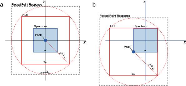
Geometry of Point Responses and Spectra. For a spectrum of width w (inner, shaded box), the portion of the point response that could appear in a spectrum is the region of interest (ROI) of size 2w × 2w (middle box). Circularly-symmetric artifacts in the point response must have a radius of at least 2^1/2w to avoid the ROI. In this paper, we plot point responses in a window (outer box) that is 2(2^1/2)w on each axis. (a) When a peak is in the center of the spectrum, at X/Y coordinates (0, 0), only the center (shaded portion) of the ROI is observed. (b) For peaks elsewhere in the spectrum, such as the corner (−w/2, −w/2) as shown here, the full point response is shifted so that it remains centered on the peak, and other parts of the ROI (shaded) become visible.

2.3. The Fourier transform of a single ring of sampling points

The sampling patterns considered here all consist of concentric rings of sampling points. Such patterns can be described as sums of individual rings of points of different radii. Because of the linearity of the FT, the point response can be calculated by transforming each ring independently, and adding together the transforms.

Thus the essential building block for analyzing concentric ring sampling patterns is the Fourier transform of a single ring of equally-spaced sampling points [28, 33, 41, 42]:

$$\begin{array}{cc}\hfill {\mathrm{P}}_{N,r_0,\varphi }& (X,Y)=2N\sum _{n=-\infty }^{\infty }{i}^n{J}_n\left(2\pi r_{0}R\right)e^{\mathit{in}\Theta +\varphi }{r}_0,\hfill \\ \hfill & n=0,\pm 2N,\pm 4N\dots \hfill \end{array}$$ [3]

where r₀ is the radius of the ring in the time domain, 2N is the number of sampling points, ϕ is the phase of the ring relative to the x axis, J_n is the Bessel function of order n, R = (X² + Y²)^1/2 and Θ = arctan Y/X. This can be derived by computing the FT in polar coordinates, with respect to azimuth, of the function describing a ring of points:

$${\rho }_{N,r_0,\varphi }(r,\theta )=\delta (r-r_0)(N∕\pi )\mathrm{III}(\theta N∕\pi +\varphi ),$$ [4]

as was shown previously [28, 33, 42]. Note the normalization factor 2N in Eq. [3], which assumes importance here.

The FT of a ring of points is thus the superposition of a series of functions that vary with radius as Bessel functions, and with azimuth as sinusoids. Two examples of such transforms are shown in Figure 2. Regardless of the number of points, the series will always include a zero-order term J₀(2πr₀R), which is circularly symmetric and gives rise to a “ripple pattern” centered on the origin of the transform. The other terms of the series have orders that are multiples of the number of sampling points. Because a Bessel function J_n(u) is approximately zero for u < n, a term of order n is approximately zero up to the distance n/πr₀ from the origin. The term rises rapidly from nothing to a peak at approximately n/πr₀, and then oscillates at increasing distances from the origin. Thus for the whole series, only the J₀ term is active at the origin, and as the distance from the origin increases, additional higher-order terms progressively begin to contribute.

Figure 2.

The Fourier Transform of a Ring of Sampling Points. Two examples are shown, each with 72 sampling points (N = 36) and phase 0, one with a radius of 9Δr, the other 14Δr. (a) Positions of the sampling points for the two rings. The axes are measured in multiples of the dwell time Δr. (b) Schematic showing the positions in the frequency domain at which the first of the higher-order Bessel terms (J₇₂) begin for the two rings, relative to the region of interest and the plotted transform size. Note that the ring of smaller radius in the time domain generates the higher-order terms of larger radii. (c) The FT of the r₀ = 9Δr ring. Note the J₀ “ripple” pattern starting from the center, with the J₇₂ term beginning close to the edge. (d) The FT of the r₀ = 14Δr ring.

2.4. Concentric Ring Sampling

We define Concentric Ring Sampling (CRS) as a method wherein the time domain is sampled on rings spaced at an equal time increment Δr. A sampling function for CRS can be constructed as a summation of m rings, with the number of sampling points on each ring j denoted as 2N_j and the phase of each ring as ϕ_j:

$$s_{\mathrm{CRS}}(r,\theta )=\sum _{j=1}^m{\rho }_{N_j,r_j,{\varphi }_j}(r,\theta ).$$ [5]

The point response (using a polar FT) follows from Eq. [3]:

$$\begin{array}{cc}\hfill S_{\mathrm{CRS}}(X,Y)& =\sum _{j=1}^m{\mathrm{P}}_{N_j,r_j,{\varphi }_j}(X,Y)\hfill \\ \hfill & =\sum _{j=1}^m\left[2N_j\sum _{n_j=-\infty }^{\infty }{i}^{n_j}{J}_{n_j}\left(2\pi r_{j}R\right)e^{{\mathit{in}}_j\Theta +{\varphi }_j}{r}_j\right],\hfill \end{array}$$ [6]

where the index n_j of the inner summation goes as 0, ±2N_j, ±4N_j,… for each ring.

An issue that arises in the processing of radially-sampled data by FT is the need to account for the unequal area density of the sampling pattern, which is accomplished in the radial case by the polar FT's factor r_j [13, 28, 43] However, when the number of points on each ring is allowed to vary, this is no longer a valid correction. Problems arise specifically from the factor 2N_j in Eq. [6], which for radial sampling is constant over all j and may be ignored, but which can vary in the general CRS case. Thus the proper area density correction for CRS becomes r_j / N_j, giving a new, corrected point response:

$$S_{\mathrm{CRS}}^{\prime }(X,Y)=\sum _{j=1}^m\left[\sum _{n_j=-\infty }^{\infty }{i}^n{J}_{n_j}\left(2\pi r_{j}R\right)e^{\mathit{in}\Theta +{\varphi }_j}{r}_j\right].$$ [7]

2.5. Data processing

Obtaining a spectrum from CRS data requires an initial processing step before the FT to convert from hypercomplex to complex data, as described previously [6, 7, 9, 28, 30]; we recommend that the reader consult [28] for a complete discussion. Briefly, linear combinations are taken of the hypercomplex FIDs to yield complex-valued data. While the original data occupies only the +x +y quadrant (N_j/2 points on ring j), the conversion calculation produces complex data for both the +x +y and −x +y quadrants, with the latter being a reflection of the former (yielding N_j total points on ring j) [28]. The transform of either quadrant of data alone would yield a spectrum with phase-twist lineshapes, but the use of both quadrants allows one to obtain purely absorptive peaks [39].

Once the complex-valued data are available, there are two options for computing the FT. One is the azimuthal form of the polar FT, which we recently described [28], involving (1) a 1-D FT of each ring, with respect to θ, followed by (2) the summation of a series of terms that vary as Bessel functions with respect to R and as sinusoids with respect to Θ, weighted according to the Fourier coefficients of the 1-D transform. Alternatively, one could employ the traditional 2-D point-by-point discrete FT, as recently suggested by Kazimierczuk and colleagues [30], adding a weighting factor as we previously noted [28]:

$$F(X,Y)=\sum _{j}f(x_j,y_j)e^{-2\pi i(x_{j}X+y_{j}Y)}\Delta A_j,$$ [8]

where the summation is over all of the available sampling points, each point j having a position (x_j, y_j) and a weight ΔA_j that is determined by the distribution of the sampling points. For CRS, this transform would be computed as:

$$F_{\mathrm{CRS}}(X,Y)=\sum _{j=1}^m\sum _{k=1}^{N_j}{f}_{\mathrm{CRS}}(r_j,{\theta }_{j,k})e^{-2\pi {\mathit{ir}}_j(X\cos {\theta }_{j,k}+Y\cos {\theta }_{j,k})}\frac{r_j}{N_j},$$ [9]

where a point j, k has a radial coordinate r_j, an azimuthal coordinate θ_j,k and a weighting factor ΔA_j,k = r_j/N_j. Eq. [9] was employed to compute the transforms in this study.

2.6. Response from the zero-order terms

If the J₀ terms of the corrected point response are separated out, one can analyze several features that are common to all CRS patterns. Each ring at a different radius r_j contributes a J₀ term with a different radial frequency of oscillation, which combine to form the series:

$$\sum _{j=1}^m{J}_0\left(2\pi r_{j}R\right)r_j.$$ [10]

This summation is of vital importance, as in essence it is responsible for the ability to obtain a valid spectrum for this type of sampling. It was studied extensively by Bracewell and Thompson [31], who found that it can be expanded as:

$$\sum _{j=1}^m{J}_0\left(2\pi r_{j}R\right)r_j=\frac{r_{\max }}{2\pi R}{J}_1\left(2\pi r_{\max }R\right)+\sum _{k=1}^{\infty }{p}_k\left(R\right),$$ [11]

where the first term on the right hand side (hereafter the “main term”) generates the peak, while the higher order terms p_k lead to replications of the peak as ringlobes at distance increments of 1/Δr from the peak. This is illustrated in Figure 3a, where we plot Eq. [10] for m = 32, after convolution with a Gaussian signal to remove truncation artifacts; the peak and the first two ringlobes are shown.

Figure 3.

Ringlobes. In CRS, the discrete sampling of the time domain with respect to r leads to a radial periodicity in the spectrum., in the form of ringlobes. (a) The zero-order terms of the CRS point response, convolved with a Gaussian signal to remove truncation artifacts. The peak and the first two ringlobes are shown. (b) A cross-section through the plot in (a). The spacing of the ringlobes is indicated. Note that the shape of each ringlobe is the shape of the peak, reduced in size and shifted in phase.

The ringlobe of order k is given by:

$$p_k\left(R\right)={\int }_0^{\pi }\left[\xi (R\cos \varphi -k∕\Delta r)+\xi (R\cos \varphi -k∕\Delta r)\right]d\varphi ,$$ [12]

where

$$\xi \left(u\right)=2r_{\max }\mathrm{sinc}\left(2r_{\max }u\right)-r_{\max }{\mathrm{sinc}}^2\left(r_{\max }u\right).$$ [13]

(ref. [31]). The ringlobes are the consequence of the discrete sampling in r: As always with the FT, discrete sampling leads to periodicity, and peak replications appear with a spacing that is the inverse of the dwell time. Because of the geometry, that periodicity takes on the form of ringlobes, rather than the direct replication of the peak seen in Cartesian sampling.

The ringlobes are generated by the interaction of the J₀ terms from different rings, at different radial frequencies, which interfere constructively at intervals of 1/Δr. Figure 3b shows a cross section through the plot of Figure 3a, illustrating the positioning and shape of the ringlobes. Bracewell and Thompson [31] showed that the ringlobes of different orders differ only by a scaling factor, the height of ringlobe k being proportional to k^−1/2. The shape of each ringlobe after the integration of Eq. [12] was found to be closely approximated (for R in the vicinity of k/Δr) by the unusual expression:

$$S_0\left(R\right)\cong 2m\sqrt{\frac{r_{\max }}{\pi R}}{\mathrm{sinc}}^{(1∕2)}[2r_{\max }R-\mathit{mk}],$$ [14]

where sinc^(1/2) represents the half-order differentiation of sinc, which is equivalent to multiplying by a window function of (2πr)^1/2 in the time domain to change the lineshape, and then shifting the phase by −45° in the frequency domain (Figure 3b). Because of the theorem that f^(a) * g = f * g^(a), we can conclude that the shape of each ringlobe reflects the shape of the original peak following apodization and a −45° phase shift, possibly with added sinc wiggles for truncated signals. The phase shift leads to a negative “skirt” on the inner side of each ringlobe, and also to a slight negative slope on the baseline inside of the ringlobe. These features are all apparent in Figure 2, where the original peak is Gaussian.

Thus if we are to avoid the intrusion of ringlobes into a CRS spectrum, we must set the spacing between sampling rings Δr to no more than 1/(2^1/2w), thereby putting the first ringlobe at 1/Δr = 2^1/2w, at the edge of the R = 2^1/2w region of interest of the point response. Assuming this condition is met, one can guarantee that the zero-order terms of Eq. [7] will lead to a correct and artifact-free spectrum, differing from a conventional spectrum only in the baseline's slight negative slope. This is a radial analog to the aliasing phenomenon in Cartesian sampling, where the spacing of points 1/Δx must be less than 1/w to prevent the intrusion of artifact peaks.

2.7. Response from the higher-order terms

We have seen that each ring of a CRS pattern contributes a J₀ term, and that the J₀ terms from the different rings combine to generate the peak. As described above in section 2.3, each ring also generates a series of higher-order terms, of the form J_n(2πr₀R)e^inΘ. These terms are purely artifactural, and ideally would be excluded from the active area of the point response completely.

Because of the fact that each term is approximately zero for R < n/πr₀, avoiding these artifacts is possible, depending upon the distribution of sampling points on the rings. Since the artifacts caused by ring j become active at a cutoff radius R_j = N_j/πr_j, the overall pattern is free from artifacts within a “clear zone” of radius R_cz = min R_j. If R_cz ≥ 2^1/2 w, there will be no artifacts within the spectrum.

Radial sampling is a specific case of CRS, and the artifacts for radially-sampled data processed by the FT follow this behavior. In radial sampling N_j is the same for all rings. While the artifacts from the innermost rings have a very large R_j—and do not appear within the active region of the point response—the artifacts from each successive ring have progressively lower R_j, eventually intruding on the active area of the point response (see Table 1 for an explicit example). The observed clear zone is governed by R_m, the cutoff for the last ring, and has a size:

$$R_{\mathrm{cz},\text{radial}}=N_{\text{radial}}∕\pi r_{\max }=\sqrt{2}{N}_{\text{radial}}w∕\pi m,$$ [15]

assuming that Δr = 1/(2^1/2w), which comes to 0.51w for N_radial = 36 spokes and m = 32 rings (this sampling pattern is plotted in Figure 4a, and the point response in Figure 5a). Increasing the number of spokes leads to a corresponding increase in R_cz, until the artifacts are eventually pushed outside of the spectrum.

Table 1.

Parameters of Sampling Patterns. All distances are relative to the spectral width w. A dwell time of Δr= 1/(2^1/2w) is assumed. The LCRS and RLCRS methods and the parameter α are defined in the text in Section 2.8. For each sampling pattern, N_j indicates the number of sampling points for ring j, which is determined according to the sampling method, while R_j indicates the corresponding artifact-free radius of the point response for that ring. The total number of points for each sampling pattern T = Σ (N_j/2 + 1). The artifact-free radius for the point response of the full sampling pattern is R_cz = min R_j.

	Radial Sampling		LCRS α = π/2		LCRS α = 1.111		RLCRS α = 1.000		RLCRS α = 0.200
j	Nj	Rj	Nj	Rj	Nj	Rj	Nj	Rj	Nj	Rj
1	36	16.21w	4	1.80 w	4	1.80 w	2	0.90 w	2	0.90 w
2	36	8.10 w	8	1.80 w	6	1.35 w	4	0.90 w	2	0.45 w
3	36	5.40 w	10	1.50 w	8	1.20 w	6	0.90 w	2	0.30 w
4	36	4.05 w	14	1.58 w	10	1.13 w	8	0.90 w	2	0.23 w
5	36	3.24 w	16	1.44 w	12	1.08 w	10	0.90 w	2	0.18 w
6	36	2.70 w	20	1.50 w	14	1.05 w	12	0.90 w	4	0.30 w
7	36	2.32 w	22	1.41 w	16	1.03 w	14	0.90 w	4	0.26 w
8	36	2.03 w	26	1.46 w	18	1.01 w	16	0.90 w	4	0.23 w
9	36	1.80 w	30	1.50 w	20	1.00 w	18	0.90 w	4	0.20 w
10	36	1.62 w	32	1.44 w	24	1.08 w	20	0.90 w	4	0.18 w
11	36	1.47 w	36	1.47 w	26	1.06 w	22	0.90 w	6	0.25 w
12	36	1.35 w	38	1.43 w	28	1.05 w	24	0.90 w	6	0.23 w
13	36	1.25 w	42	1.45 w	30	1.04 w	26	0.90 w	6	0.21 w
14	36	1.16 w	44	1.41 w	32	1.03 w	28	0.90 w	6	0.19 w
15	36	1.08 w	48	1.44 w	34	1.02 w	30	0.90 w	6	0.18 w
16	36	1.01 w	52	1.46 w	36	1.01 w	32	0.90 w	8	0.23 w
17	36	0.95 w	54	1.43 w	38	1.01 w	34	0.90 w	8	0.21 w
18	36	0.90 w	58	1.45 w	40	1.00 w	36	0.90 w	8	0.20 w
19	36	0.85 w	60	1.42 w	44	1.04 w	38	0.90 w	8	0.19 w
20	36	0.81 w	64	1.44 w	46	1.04 w	40	0.90 w	8	0.18 w
21	36	0.77 w	66	1.41 w	48	1.03 w	42	0.90 w	10	0.21 w
22	36	0.74 w	70	1.43 w	50	1.02 w	44	0.90 w	10	0.20 w
23	36	0.70 w	74	1.45 w	52	1.02 w	46	0.90 w	10	0.20 w
24	36	0.68 w	76	1.43 w	54	1.01 w	48	0.90 w	10	0.19 w
25	36	0.65 w	80	1.44 w	56	1.01 w	50	0.90 w	10	0.18 w
26	36	0.62 w	82	1.42 w	58	1.00 w	52	0.90 w	12	0.21 w
27	36	0.60 w	86	1.43 w	60	1.00 w	54	0.90 w	12	0.20 w
28	36	0.58 w	88	1.41 w	64	1.03 w	56	0.90 w	12	0.19 w
29	36	0.56 w	92	1.43 w	66	1.02 w	58	0.90 w	12	0.19 w
30	36	0.54 w	96	1.44 w	68	1.02 w	60	0.90 w	12	0.18 w
31	36	0.52 w	98	1.42 w	70	1.02 w	62	0.90 w	14	0.20 w
32	36	0.51 w	102	1.43 w	72	1.01 w	64	0.90 w	14	0.20 w
Rcz		0.51 w		1.41 w		1.00 w		0.90 w		0.18 w
T	608		844		602		528		119

Figure 4.

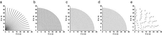
CRS Sampling Patterns. All patterns shown for m = 32 rings. The LCRS and RLCRS methods and the parameter α are defined in the text in Section 2.8. (a) Radial sampling, N_radial = 36. (b) LCRS, α = π/2. (c) LCRS, α = 1.111. (d) RLCRS, α = 1.0. (e) RLCRS, α = 0.2.

Figure 5.

Point Responses for CRS Patterns. For each pattern, a contour plot at ∼3% of peak height and a stacked plot viewed from above are given. The LCRS and RLCRS methods and the parameter α are defined in the text in Section 2.8. (a) Radial sampling. Moving out from the center, one encounters the first artifacts at 0.51w, where the J₇₂ term becomes active. In the stacked plot, this appears as a transition from ripples to ridges. The contour plot makes the radial dependence on a Bessel function more apparent, showing that the response oscillates with respect to R. At ∼w, the number of ridges doubles, and a new ring of intensity is encountered as the J₁₄₄ term becomes active. Finally, at 2^1/2w is the first ringlobe. (b) LCRS with α = π/2. There are no artifacts inside of the first ringlobe. (c) LCRS α = 1.111. Although there are artifacts inside the first ringlobe, due to their angular dependence, they are almost entirely outside the region of interest (ROI). (d) RLCRS α = 1.000 (phases randomized). The artifacts intrude on the ROI, but still occupy less of the spectrum than with radial sampling. (e) RLCRS a = 0.200 (phases randomized). The artifacts occupy all of the spectrum and appear like random noise.

Beyond R_cz, the higher-order terms are sinuisoidally dependent on azimuth, which becomes important for determining the nature of the artifacts. Again taking the radial case as an example, for R > R_cz,radial the artifacts are sinusoidal with respect to Θ, with 2N_radial cycles around the circle. Because each ring has the same N_j = N_radial and the same relative phase ϕ _j = 0, the artifacts from the different rings have the same azimuthal frequencies and phases, and form the familiar set of ridge artifacts [28].

2.8. Optimization of the distribution to minimize artifacts

The portion of the spectrum affected by artifacts can be reduced by distributing the sampling points to maximize R_cz. For a given number of sampling points, the maximum R_cz is achieved by setting N_j such that all R_j are approximately equal. To obtain R_cz equal to a given target size Rtarget most efficiently, the distribution should be designed to give nearly equal R_j = Rtarget for all rings.

Letting Rtarget be the desired size of the clear zone, the distribution with equal R_j for all rings is achieved with the equation:

$$N_j=2\lceil R_{\text{target}}\pi r_j∕2\rceil ,$$ [16]

where we require N_j/2, the number of physically observed sampling points prior to reflection into the −x +y quadrant (see section 2.5 above), to be an integer (the ceiling brackets round the enclosed quantity up to the next integer). This distribution has the property that the number of points on each ring grows as a linear function of the ring number, which becomes clear when Eq. [16] is rewritten as:

$$\frac{N_j}{2}=\lceil \frac{\pi R_{\text{target}}j}{2\sqrt{2}w}\rceil =\lceil \alpha j\rceil ,\left(\alpha \equiv \frac{\pi R_{\text{target}}}{2\sqrt{2}w}\right).$$ [17]

We designate sampling patterns derived from Eq. [16]/[17] linearly-increasing concentric ring sampling (LCRS).

The total number of physically-observed sampling points needed for LCRS for a given α parameter is:

$$T_{\alpha }=\sum _{j=1}^m\lceil \alpha j\rceil ,$$ [18]

which is approximated to within αm points by removing the ceiling brackets:

$$T_{\alpha }\approx \sum _{j=1}^m\alpha j=\frac{1}{2}\alpha m(m+1).$$ [19]

Obtaining R_target = 2^1/2w, which is the minimum that would guarantee that an artifact term cannot become active within a spectrum, requires that α = π/2. The sampling pattern for this case with m = 32 rings is plotted in Figure 4b, and the N_j and R_j values are given in Table 1. Note from Table 1 that the rings all have R_j ≈ 2^1/2w as intended. The point response is plotted in Figure 5b; the first ringlobe is visible as a ring around the outside of the pattern, and otherwise only the peak and the truncation artifacts of the main term are observed. However, α = π/2 LCRS requires a fairly large number of sampling points (844 in the case of m = 32 rings), representing only a small savings over the conventional sampling, and it would be desirable to find approaches requiring fewer sampling points. While smaller values of α would potentially lead to the intrusion of artifacts in the spectrum, whether this is problematic would depend on the nature of those artifacts.

2.9. The form of the artifacts in LCRS, outside the clear zone

In a case of LCRS with R_cz < 2^1/2w, the form of the observed artifacts becomes an important consideration. For distributions with R_j = R_cz, one expects the artifacts to peak at approximately the same radial coordinate R_cz. This would lead to a ringlobe of artifactural intensity at R_cz, were it not for the additional modulation of each artifact term with respect to Θ, by the factor e^inΘ. For α = 1.0, and assuming that each ring is measured with the same phase ϕ_j = 0, the result at R_cz is not a ringlobe but rather a truncated 1-D Fourier series with respect to Θ:

$$S_{\alpha =1.0}^{\prime }(R_{\mathrm{cz}},\Theta )\approx \sum _{n=1}^m(\cos 4n\Theta +i\sin 4n\Theta ),$$ [20]

which is written as an approximation since the radial dependencies of the J_n(2πr_jR) functions are not exactly the same for all orders of J_n. Because the waves generated by the different rings of sampling points have different angular frequencies, they interfere destructively for most values of Θ, but reinforce at intervals of ΔΘ = π/2, with only small truncation wiggles in between. The constraint that N_j/2 be an integer causes the angular frequencies of the individual rings to be multiples of 4, leading to the periodicity in Θ of 2π divided by 4. The resulting artifact peaks somewhat resemble aliasing artifacts in Cartesian sampling regimes, although with distorted peak shapes.

Provided that all rings have the same phase ϕ_j = 0, the result for other values of α:

$$S_{\alpha \ne 1.0}^{\prime }(R_{\mathrm{cz}},\Theta )\approx \sum _{n=1}^m(\cos 4\lceil \alpha n\rceil \Theta +i\sin 4\lceil \alpha n\rceil \Theta ),$$ [21]

is very similar. By the definition of LCRS, the number of sampling points per ring is always an integer multiple of four, and the point response will thus always have the four strong axial artifact peaks at intervals of π/2, as for α = 1.0. The effect of α ≠ 1.0 on the response is primarily to change the shapes of the wiggles between the artifact points slightly, and in some cases to introduce additional small artifacts close to the axes.

The fact that the only significant artifacts in LCRS spectra are found on the axes suggests that one could obtain an almost perfect spectrum using a distribution with R_target = w, which would require α = 2^1/2π/4 ≈ 1.111. The point response for this pattern is shown in Figure 5c, while the point distribution is given in Table 1 and plotted in Figure 4c. Table 1 shows that the artifacts can be expected to start at the radius R_cz = w. The ΔΘ = π/2 periodicity leads to artifact peaks along the axes at R = R_cz that are ∼28% of the true peak height. Two additional artifact peaks are found next to each axial artifact, at ∼5% of peak height. For other Θ, however, the artifacts are <1% of the peak height up to the start of the first J₀ ringlobe at R = 1/Δr. All significant artifacts are found along and close to the axes, and therefore outside the 2w × 2w region of interest. This distribution could be considered the most efficient artifact-free LCRS pattern possible.

Using the LCRS approach with even fewer sampling points (α < 2^1/2π/4) requires accepting artifacts of one form or another, but those artifacts can be made more tolerable by changing the approach slightly. The distribution described above concentrates the majority of the artifacts along the axes, which is generally only acceptable if those concentrated artifacts can be kept beyond the edge of the region of interest. However, when the sampling is insufficient to achieve R_cz > w, instead of concentrating the artifacts along the axes, it is advantageous to distribute them as evenly as possible in Θ, giving them the smallest impact on the resulting spectrum. This can be accomplished by randomizing the phases ϕ_j of the sampling rings, in a phase-randomized LCRS (RLCRS). Note that this phase parameter does not refer to the phase of the signals but rather the relative orientations of the sampling rings. The resulting artifacts begin sharply at R_cz and are nearly evenly distributed about Θ, fluctuating in a manner similar to random noise. When randomizing the phases it is necessary to apply an additional correction to the point-by-point weighting in the DFT calculation (Eq. [9]), to account for the fact that the points closest to the axes do not have the same uniform 1/N_j area density as the other points.

An example of RLCRS with randomized phases is shown in Figure 4d, for α = 1.00. The artifacts range up to 10% of the peak height (comparable to radial sampling), but have an appearance that is quasi-random. This figure points to one minor consequence of the method that should be noted: Randomizing the phase disturbs the symmetry of the sampling pattern following reflection into the −x +y plane, leading to minor baseline disruption within the clear zone, albeit at < 1% of peak height. While distortion of the peak shape from this change is theoretically possible, we have not been able to detect it, suggesting that the distortion is less than the calculation precision. The α = 1 sampling pattern is plotted in Figure 4d, and the relevant parameters are given in Table 1.

The much more extreme case of α = 0.2, which involves a 80% reduction in measurement time over the artifact-free LCRS case, has also been included in Table 1 and Figure 4-6. In this case, the artifacts have assumed the appearance of random noise distributed throughout the plane at a level of ∼10% of peak height.

Figure 6.

Experimental Results. Shown is a representative N/CO plane from the 3-D HNCO spectrum of GB1 (HN=7.95 ppm). (a) Cartesian control at the same resolution as the CRS spectra. (b) Radial sampling. Note that almost all of the baseline is filled with ridge artifacts. (c) LCRS α = π/2. The spectrum is indistinguishable from the Cartesian, except for some ripple truncation artifacts (<1%). (d) LCRS α = 1.111. This spectrum is also nearly identical to the control. (e) RLCRS α = 1.000. The standard CRS artifacts from higher-order Bessel terms are visible, in the farthest corner to the left, at a level of ∼5% of peak height. The randomization of the phases disturbs the symmetry of the sampling pattern upon reflection of the data, leading to a variation in the baseline of 1-2% of peak height. (f) RLCRS a = 0.200. In this extreme case, determined with only 120 sampling points, the artifacts cover the plane and appear like random noise. However, the resolution is the same as for the other sampling patterns. (g) A truncated version of the Cartesian control, with the same number of points as in the RLCRS a = 0.200 experiment. Reducing the number of points in Cartesian sampling without introducing aliased peaks requires a severe loss of resolution. By comparison, reducing the measurement time for LCRS/RLCRS preserves resolution but introduces low-level artifacts.

2.10. Sensitivity considerations

The weighting factors used to correct for unequal area density in the sampling pattern can have an effect on the sensitivity of the resulting spectrum. To quantitate these effects, we apply the principles of signal averaging while assuming a non-decaying signal and a standard Gaussian noise distribution, to reduce the complexity of the analysis. It should be noted that we refer here to the true noise level, i.e. the noise that would be observed in the clear zone of the spectrum. With very low α, or for many cases of radial sampling, the apparent noise would be larger due to the presence of artifacts. For general CRS, the signal and noise levels for ring j (σ_j and η_j, respectively) would be:

$${\sigma }_j={\sigma }_0{N}_j,{\eta }_j={\eta }_0\sqrt{N_j},$$ [22]

where σ₀ and η₀ are the signal level and the standard deviation of the noise distribution, respectively, for a single sampling point. The signal level σ of the spectrum is not dependent on the sampling pattern, due to the normalization by 1/N_j:

$$\sigma =\sum _{j=1}^m\frac{r_j}{N_j}{\sigma }_j={\sigma }_0\sum _{j=1}^{m}j=\frac{1}{2}{\sigma }_{0}m(m+1),$$ [23]

while the standard deviation of the noise η does depend on the distribution of sampling points among the rings:

$$\eta =\sqrt{\sum _{j=1}^m{\left(\frac{r_j}{N_j}\right)}^2{\eta }_j^2}={\eta }_0\sqrt{\sum _{j=1}^m\frac{r_j^2}{N_j}}.$$ [24]

To facilitate the comparison of results from different sampling patterns, it will be helpful to define a relative sensitivity measure ν :

$$\nu =\frac{(\sigma ∕\eta )}{\sqrt{2T}({\sigma }_0∕{\eta }_0)},$$ [25]

which is the ratio of the signal-to-noise for an experimental sampling pattern to that of the Cartesian sampling pattern with the same number of sampling points. Note that in this discussion we always count the number of data points and assess the sensitivity per point σ ₀/η ₀ after conversion from hypercomplex to complex data (necessitating the factor of 2 in the denominator of Eq. [25], since T is defined in Eq. [18] as the number of points before reflection).

First, we consider the result for radial sampling. In this case, the noise would be:

$$\begin{array}{cc}\hfill {\eta }_{\text{radial}}& =\frac{{\eta }_0}{\sqrt{N_{\text{radial}}}}\sqrt{\sum _{j=1}^m{j}^2}\hfill \\ \hfill & =\frac{{\eta }_0}{\sqrt{N_{\text{radial}}}}\sqrt{\frac{1}{6}m(m+1)(2m+1)},\hfill \end{array}$$ [26]

leading to a signal to noise ratio of:

$$\frac{\sigma }{{\eta }_{\text{radial}}}=\sqrt{N_{\text{radial}}}\left(\sqrt{\frac{3m(m+1)}{2(2m+1)}}\right)({\sigma }_0∕{\eta }_0),$$ [27]

and a relative sensitivity of:

$${\nu }_{\text{radial}}=\frac{\sigma ∕{\eta }_{\text{radial}}}{\sqrt{m{N}_{\text{radial}}}({\sigma }_0∕{\eta }_0)}=\sqrt{\frac{3m(m+1)}{2(2m+1)}}.$$ [28]

The relative sensitivity for the same time thus comes to 87.3% for m = 32 rings, and approaches a value of 3^1/2/2 ≈ 86.6% in the limit of large m. This ∼13% sensitivity loss for radial sampling is a consequence of the reweighting of the sampling points in the FT by the function r_j, which corrects for the uneven distribution of the points in the time domain. Interestingly, this sensitivity loss is not affected by the number of radial spokes N_radial.

The LCRS case gives somewhat different results. Approximating the number of points on each ring 2⌈αj⌉ as 2α j, one obtains a noise level of:

$$\begin{array}{cc}\hfill {\eta }_{\alpha }& ={\eta }_0\sqrt{\sum _{j=1}^m\frac{r_j^2}{2\lceil \alpha j\rceil }}\hfill \\ \hfill & \approx {\eta }_0\sqrt{\frac{1}{2\alpha }\sum _{j=1}^{m}j}={\eta }_0\sqrt{\frac{1}{2\alpha }\left[\frac{1}{2}m(m+1)\right]}.\hfill \end{array}$$ [29]

The signal to noise ratio is thus:

$$\frac{\sigma }{{\eta }_{\alpha }}=\sqrt{2\alpha }\left(\sqrt{\frac{1}{2}m(m+1)}\right)({\sigma }_0∕{\eta }_0),$$ [30]

and the sensitivity relative to Cartesian sampling is:

$$\begin{array}{cc}\hfill {\nu }_{\alpha }& =\frac{\sigma ∕{\eta }_{\alpha }}{\sqrt{2T_{\alpha }}({\sigma }_0∕{\eta }_0)}\hfill \\ \hfill & =\frac{\sqrt{2\alpha }\left(\sqrt{\frac{1}{2}m(m+1)}\right)}{\sqrt{2\alpha }\left(\sqrt{\frac{1}{2}m(m+1)}\right)}=1.\hfill \end{array}$$ [31]

Thus we find that LCRS has identical sensitivity to Cartesian sampling in all cases, for the same measurement time.

3. Results

To demonstrate the LCRS approach, we collected 3-D HNCO spectra from the B1 domain of protein G (GB1) using the α = π/2, α = 1.111, α = 1.000 and α = 0.200 LCRS patterns described above, which we compare to radial sampling for a similar number of sampling points, and to conventional Cartesian sampling at the same resolution (however, see the Discussion section regarding resolution). The spectral width was w = 2000 Hz for both the N and the CO axes, requiring that the spacing between rings Δr be 1/(2^1/2w) = 1/(2^1/2 × 2000) ≈ 2900 Hz. The CRS spectra were collected with m = 32 rings of points. The distributions of sampling points in the LCRS patterns are given in Table 1 and Figure 4; they required 844, 602, 528 and 119 points, respectively. The Cartesian and radial controls used 1024 and 608 points, respectively.

The LCRS spectra correctly reproduce all peaks in the conventional spectrum, and with the same resolution. Figure 6 shows stacked plots of a representative plane from this spectrum, as reproduced by each of these methods. The α = π/2 spectrum is indistinguishable from the conventional. Importantly, however, the α = 1.111 is also nearly identical to the conventional result, despite having α < π/2. By comparison, a radially sampled experiment with projections at 5° increments (N_radial = 36 measured spokes, after reflection), collected in the same measurement time as the α = 1.111 spectrum, shows substantial artifacts covering a large portion of the plane (starting at a distance of 0.51w = 1020 Hz from each peak).

Reducing the number of sampling points for m = 32 rings below 602 points (i.e. α < 1.111) requires introducing the RLCRS method described above. The result for α = 1.0 shows artifacts that reach as much as 10% of peak height, but which do not begin until a distance of 0.90w = 1800 Hz. They are therefore observed only for peaks that are near the edges of the spectrum, and when they are observed, they are found only towards the corners, occupying a much smaller part of the spectrum than in radial sampling. Additionally, because of the phase randomization, their form appears like random noise, rather than the ridge shapes found in the radial spectra. The large size of the artifact-free zone around each peak substantially reduces the chance of the artifacts from any one peak interfering with the shapes of other peaks, as would be the case for radial sampling. The α = 0.2 result also shows artifacts at 10% of peak height, but in this case covering almost the entire plane, and appearing as random noise. The resolution of the peak is the same as in the cases with more sampling points, however. For comparison, in Figure 6g the Cartesian data were truncated to have the same number of sampling points as in the RLCRS α = 0.2 experiment, showing how one can reduce the measurement time in LCRS/RLCRS while preserving resolution (at the expense of low-level artifacts), while reducing the measurement time for Cartesian sampling requires a severe loss of resolution.

4. Discussion

4.1. Dwell time and resolution

Because CRS methods produce ringlobe artifacts at radial intervals of 1/Δr, it is necessary to set Δr = 1/(2^1/2w), rather than the usual 1/w of Cartesian sampling. This reduces the potential efficiency of the method, since the resolution achieved for a given number of rings m is 1/mΔr = 2^1/2w/m instead of w/m. We have previously enhanced the efficiency of radial sampling by adjusting Δr depending on the azimuth θ, according to the equation:

$$\Delta r_{\theta }=\frac{1}{w(\cos \theta +\sin \theta )},$$ [32]

(assuming here a square spectrum; ref. [10]). This equation maximizes the resolution in each direction, making it possible to obtain spectra of very high resolution on the orthogonal axes without the intrusion of ringlobe artifacts. While we did not apply that technique here, to simplify the theoretical analysis, it should nonetheless be feasible to apply this in practice for any CRS method, including LCRS. This would allow one to obtain a spectrum at a higher resolution than is here achieved. Our previous work suggests that any distortion caused by applying Eq. [32] would be minor [13, 44]; a full quantitative analysis is in progress, along with an analysis of cases with unequal spectral widths on the two axes.

4.2. Comparison of sampling methods

Comparing the two CRS approaches described here, LCRS and radial sampling, is somewhat complicated due to the number of variables involved and their complex interdependencies. It is particularly challenging to address the relative efficiencies of the methods, in terms of the results achieved for a given measurement time. However, the analysis becomes tractable if one fixes a “target value” for at least one parameter, and evaluates the relative performance of the two methods when optimized to achieve the target. We will consider two such cases here: In the first, we seek to achieve a fixed resolution, while in the second, we seek to achieve an artifact-free spectrum. For the latter, it is also meaningful to make a comparison with Cartesian sampling.

4.2.1. Comparison of LCRS and radial sampling for a fixed target resolution

The choice of the number of rings m directly controls the final resolution of the experiment, which is equal to the inverse of the maximum evolution time 1/r_max = 1/mΔr = 2^1/2w/m, assuming a square spectrum. Note that the resolution in CRS is the same in all directions, since the maximum evolution time is the same in all directions. For the analysis below, given a specific target value of m, we vary the number of sampling points T, a direct surrogate of the measurement time, and evaluate the effects on artifacts and sensitivity.

The first parameter to consider is the size of the artifact-free radius R_cz, measured relative to the spectral width w. With m fixed, the number of points for LCRS is adjusted by varying α. Using the approximation in Eq. [19], we find that R_cz is:

$$R_{\mathrm{cz},\mathrm{LCRS}}=\frac{4\sqrt{2}\mathit{wT}}{\pi m(m+1)}.$$ [33]

In the case of radial sampling, when m is fixed, the number of measurement points is determined by the choice of the number of radial spokes N_radial/2. The form of the artifact free radius with respect to T turns out to be surprisingly similar to that of LCRS, the difference being a factor of two:

$$R_{\mathrm{cz},\text{rad}}=\frac{2\sqrt{2}\mathit{wT}}{\pi m^2}.$$ [34]

These curves are plotted in Figure 7a, assuming m = 32. In terms of the artifact-free radius of the spectrum, LCRS is two-fold more efficient than radial sampling.

Figure 7.

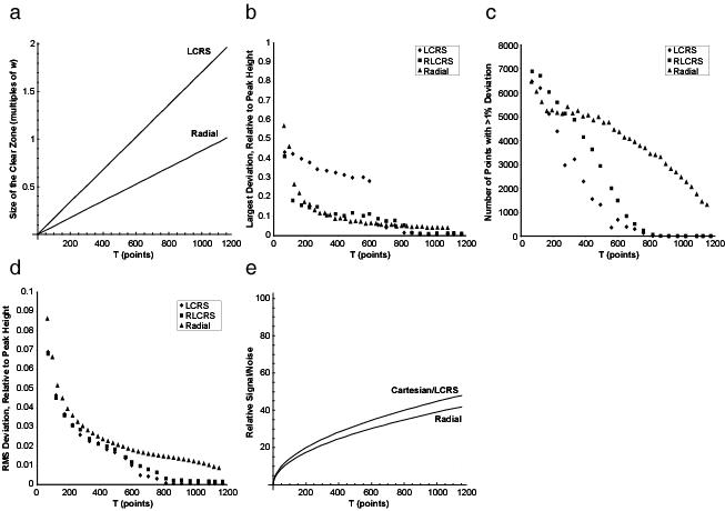
Comparison of LCRS with Radial Sampling at a Fixed Resolution. All graphs are for m = 32 rings and Δr = 1/(2^1/2w). (a) Theoretical R_cz vs. the total points T. The size of the clear zone (R_cz) is twice as large with LCRS as for radial for the same measurement time. (b) The size of the largest artifact vs. T. In LCRS, the largest artifact is substantial as the number of points increases until α = 1.111 (here ∼600 points), where the large axial artifacts pass outside the spectrum. For α > 1.111 LCRS has the smallest artifacts. For α < 1.111, it is best to use the phase randomized version of LCRS, with artifact sizes comparable to radial, but with much less area of the spectrum occupied by the artifacts than with radial sampling. (c) Number of points with >1% deviation vs. T. The LCRS methods have a much smaller area of the spectrum occupied with artifacts. (d) RMS deviation vs. T. The RMS deviation of the LCRS spectra is consistently lower than for radial sampling. (e) Theoretical signal/noise relative to that of a single measurement point vs. T. The sensitivity of LCRS is equal to Cartesian sampling, and ∼13% better than radial sampling.

Additional insight into the spectral quality can be gained by examining the deviation of the spectrum from the true spectrum as a function of the number of sampling points. Figure 7b-d plot the largest deviation, number of points with a deviation >1%, and the RMS deviation for the whole spectrum, respectively, as functions of T.

The size of the largest artifact shows the expected sharp drop for LCRS at α = 1.111, as the large axial artifacts are pushed beyond the edge of the spectrum (with a tail, however, due to the somewhat long tails of these axial artifact peaks). The other two measures, however, best illustrate the advantages of LCRS, showing a significantly smaller RMS deviation, and far fewer points with >1% deviation. The phase randomization approach avoids large artifacts for α < 1.111, but for α > 1.111 LCRS has lower artifacts than RLCRS. We can therefore conclude from Figures 7a-d that (1) artifact-free spectra can be obtained with far fewer points in LCRS than with radial sampling, and (2) when artifacts are observed in LCRS, they occupy proportionately less area of the spectrum, and are smaller, than for radial sampling in the same measurement time.

LCRS is also superior to radial sampling in terms of sensitivity when seeking a fixed resolution. The signal-to-noise ratios of the two methods are:

$$\frac{\sigma }{{\eta }_{\mathrm{LCRS}}}=\sqrt{2T},$$ [35]

for LCRS and:

$$\frac{\sigma }{{\eta }_{\text{radial}}}=\sqrt{\frac{3T(m+1)}{1+2m}},$$ [36]

for radial sampling. These curves are plotted in Figure 7e for m = 32. LCRS has the same sensitivity as Cartesian sampling, for any choice of measurement time. By comparison, radial sampling trails Cartesian sampling and LCRS in sensitivity by ∼13%.

4.2.2. Comparison of LCRS, radial sampling and Cartesian sampling for an artifact-free spectrum

We now compare the results when T is varied, and the other parameters are adjusted to obtain an “artifact-free” spectrum. We will here consider an LCRS spectrum with R_cz = w (α = 1.111) to be effectively free of artifacts >1% of peak height, while for radial sampling we require that R_cz = 2^1/2w, since radial artifacts are equally strong for all Θ. Thus in the LCRS case, we constrain α and adjust m, with T following according to Eq. [19]:

$$m=\frac{1}{2}\left(\sqrt{\frac{8T}{\alpha }+1}-1\right).$$ [37]

For radial sampling, m and N_radial are adjusted simultaneously to maintain the fixed ratio N_radial = πm, according to the relationships:

$$m=\sqrt{\frac{2T}{\pi }},N_{\text{radial}}=\sqrt{2\pi T}.$$ [38]

If the resolution 1/r_max = 1/mΔr is plotted as a function of T, one obtains the curves in Figure 8a. Here, we also include a Cartesian curve based on a resolution along each axis of w/T^1/2, assuming a square spectrum of width w, a dwell time on each axis of Δr = 1/w and T^1/2 × T^1/2 sampling points. Even without the use of Eq. [32], we find that the resolution of LCRS when seeking an artifact-free spectrum tracks with that of conventional sampling: The same maximum evolution time on each axis, and therefore the same resolution, is achieved for the same overall number of points. By comparison, radial sampling requires a larger number of sampling points than either LCRS or Cartesian sampling to obtain an artifact-free spectrum at the same resolution.

Figure 8.

Comparison of LCRS with Radial and Cartesian Sampling, When Configured to Obtain an Artifact-Free Spectrum. (a) Theoretical resolution vs. total points T. The resolution of LCRS and Cartesian sampling for the same measurement time are almost identical, and superior to that of radial sampling. (b) Theoretical signal/noise relative to that of a single sampling point vs. T. The sensitivity of radial sampling lags behind the other two methods.

In terms of sensitivity under these conditions, once again we find that LCRS is superior to radial sampling, and on par with Cartesian. Using Eq. [37] and [38], we derive the signal-to-noise per sampling point for LCRS with α fixed to be:

$$\frac{\sigma }{{\eta }_{\mathrm{LCRS}}}=\sqrt{2T},$$ [39]

which is the same as for Cartesian sampling, while for radial sampling under these constraints it is:

$$\frac{\sigma }{{\eta }_{\text{radial}}}=\sqrt{\frac{3T(\pi -\sqrt{2\pi T}-4T)}{\pi -8T}}.$$ [40]

These curves are plotted in Figure 8b.

4.3. Extension to higher dimensionality

The LCRS method should extend readily to higher-dimensionality spectra. Instead of rings, one would have concentric shells or spheres of sampling points. As with radial sampling, one expects the benefits of LCRS to be greater for higher-dimensional cases than for 3-D.

4.4. Comparison to other sparse sampling methods

In this study, we have not attempted to compare LCRS with other forms of sparse sampling, such as the exponentially-weighted random sampling methods. While our approach has been to design a sampling pattern that would place its artifacts outside the field of view whenever possible, in the extreme case of RLCRS with very small α the methods share in common the effect of spreading the artifacts as evenly as possible over the plane, in a form that resembles random noise. In the exponential sampling approach, nonlinear processing methods are typically used to reduce this artifact level substantially; the literature suggests that with FT processing the artifact levels for the two sampling approaches would be similar [20]. It would be worthwhile in the future to develop a formulation of maximum entropy reconstruction for polar coordinates, which might significantly reduce the artifact levels, and which would also permit a direct comparison of the two sampling approaches to be made. A comparison to other approaches suggests that the CRS methods could be further optimized to improve resolution and sensitivity by taking into account the signal envelope [45].

While this paper was in review, a study by Kazimierczuk et al. presenting results for FT processing of randomly distributed sampling points was published [46]. It would be interesting to compare all of these methods in the future.

5. Conclusions

We have described a generalization of radial sampling that we call concentric ring sampling (CRS), and have presented a comprehensive analytical treatment of the results, including spectral quality and sensitivity. CRS methods reproduce peaks quantitatively, although possibly with artifacts, depending on the number of points used. The new LCRS method introduced here can produce an artifact-free spectrum with equal measurement time and sensitivity to Cartesian sampling. Further, in cases of reduced measurement time where artifacts are present, the phase-randomized RLCRS result will have fewer and smaller artifacts than radial sampling for the same number of sampling points. Additionally, the sensitivity of LCRS and RLCRS is better than that of radial sampling. We expect the approach employed here to serve as the basis for developing sampling methods of even greater efficiency in the future.

6. Methods

Point responses and simulated spectra were calculated from the analytical equations using custom C++ programs, which are available upon request. For the phase-randomized RLCRS method, the phase of each ring ϕ_j was set to a number between 0 and π/2 chosen at random and with uniform probability via the Boost MT19937 pseudo-random number generator and the Boost uniform variate generator (Boost Random Number Library, Boost C++ Libraries, Release 1.32, http://www.boost.org/libs/random). FTs of simulated time domain data were computed using Eq. [9]. All data points on a ring received the same weight r_j/N_j, except for phase-randomized RLCRS patterns, in which the weights of the two points on each ring closest to the x and y axes were adjusted depending on the phase of the ring, in proportion to the relative area of the plane attributable to each point. The assessments of artifacts in Section 4.2 were determined by subtracting the normalized simulated point responses with different parameters from a reference point response of LCRS α = π/2, which shows only the J₁ truncation artifacts, to yield a difference spectrum. The relevant statistics were then computed from this difference spectrum.

NMR data were collected on a Varian INOVA 600 MHz spectrometer equipped with a triple-resonance cryoprobe with Z-axis gradients. A 2 mM sample of GB1, uniformly-labeled with ¹³C and ¹⁵N, was used, and all experiments were recorded at 25°C. The schedules of sampling points for CRS experiments were as given in Table 1 and Figure 4, with a spectral width w of 2000 Hz and a dwell time Δr = 0.345 ms. CRS experiments were collected with four transients per FID, for total measurement times: radial, 3.67 hrs.; LCRS α = π/2, 5.08 hrs.; LCRS α = 1.111, 3.63 hrs.; RLCRS α = 1.0, 3.18 hrs; RLCRS α = 0.2, 0.64 hrs. Data were initially processed using PRSP [44] and NMRPipe [47]. The final 3-D HNCO spectra were computed by a custom C++ program implementing Eq. [9], which is available upon request. Data were apodized using cosine functions in the N and CO dimensions before transformation. Cartesian data were collected with 32 complex points on each indirect axis and the same dwell time of 0.345 ms, for a total time of 6.17 hrs. for the same number of transients as in the CRS cases, and were processed using NMRPipe.

References

- 1.Nagayama K, Bachmann P, Wüthrich K, Ernst RR. The Use of Cross-Sections and of Projections in Two-dimensional NMR Spectroscopy. J. Magn. Reson. 1978;31:133–148. [Google Scholar]
- 2.Bodenhausen G, Ernst RR. The Accordion Experiment, a Simple Approach to Three-Dimensional Spectroscopy. J. Magn. Reson. 1981;45:367–373. [Google Scholar]
- 3.Szyperski T, Wider G, Bushweller JH, Wuthrich K. 3D 13C-15N-Heteronuclear Two-Spin Coherence Spectroscopy for Polypeptide Backbone Assignments in 13C-15N-Double-Labeled Proteins. J. Biomol. NMR. 1993;3:127–132. doi: 10.1007/BF00242481. [DOI] [PubMed] [Google Scholar]
- 4.Simorre JP, Brutscher B, Caffrey MS, Marion D. Assignment of NMR Spectra of Proteins Using Triple-resonance Two-dimensional Experiments. J. Biomol. NMR. 1994;4:325–334. doi: 10.1007/BF00179343. [DOI] [PubMed] [Google Scholar]
- 5.Ding K, Gronenborn AM. Novel 2D Triple-Resonance NMR Experiments for Sequential Resonance Assignments of Proteins. J. Magn. Reson. 2002;156:262–268. doi: 10.1006/jmre.2002.2537. [DOI] [PubMed] [Google Scholar]
- 6.Kozminski W, Zhukov I. Multiple Quadrature Detection in Reduced Dimensionality Experiments. J. Biomol. NMR. 2003;26:157–166. doi: 10.1023/a:1023550224391. [DOI] [PubMed] [Google Scholar]
- 7.Kim S, Szyperski T. GFT NMR, a New Approach To Rapidly Obtain Precise High-dimensional NMR Spectral Information. J. Am. Chem. Soc. 2003;125:1385–1393. doi: 10.1021/ja028197d. [DOI] [PubMed] [Google Scholar]
- 8.Freeman R, Kupče E. New Methods for Fast Multidimensional NMR. J. Biomol. NMR. 2003;27:101–113. doi: 10.1023/a:1024960302926. [DOI] [PubMed] [Google Scholar]
- 9.Kupče E, Freeman R. Reconstruction of the three-dimensional NMR spectrum of a protein from a set of plane projections. J. Biomol. NMR. 2003;27:383–387. doi: 10.1023/a:1025819517642. [DOI] [PubMed] [Google Scholar]
- 10.Coggins BE, Venters RA, Zhou P. Generalized Reconstruction of n-D NMR Spectra from Multiple Projections: Application to the 5-D HACACONH Spectrum of Protein G B1 Domain. J. Am. Chem. Soc. 2004;126:1000–1001. doi: 10.1021/ja039430q. [DOI] [PubMed] [Google Scholar]
- 11.Xia Y, Zhu G, Veeraraghavan S, Gao X. (3,2)D GFT-NMR Experiments for Fast Data Collection from Proteins. J. Biomol. NMR. 2004;29:467–476. doi: 10.1023/B:JNMR.0000034352.75619.3f. [DOI] [PubMed] [Google Scholar]
- 12.Freeman R, Kupče E. Distant Echoes of the Accordion: Reduced Dimensionality, GFT-NMR, and Projection-Reconstruction of Multidimensional Spectra, Concept. Magnetic. Res. 2004;23A:63–75. [Google Scholar]
- 13.Coggins BE, Venters RA, Zhou P. Filtered Backprojection for the Reconstruction of a High-Resolution (4,2)D CH3-NH NOESY Spectrum on a 29 kDa Protein. J. Am. Chem. Soc. 2005;127:11562–11563. doi: 10.1021/ja053110k. [DOI] [PubMed] [Google Scholar]
- 14.Hiller S, Fiorito F, Wüthrich K, Wider G. Automated Projection Spectroscopy. Proc. Natl. Acad. Sci. U. S. A. 2005;102:10876–10881. doi: 10.1073/pnas.0504818102. [DOI] [PMC free article] [PubMed] [Google Scholar]
- 15.Eghbalnia HR, Bahrami A, Tonelli M, Hallenga K, Markley JL. High-resolution Iterative Frequency Identification for NMR as a General Strategy for Multidimensional Data Collection. J. Am. Chem. Soc. 2005;127:12528–12536. doi: 10.1021/ja052120i. [DOI] [PMC free article] [PubMed] [Google Scholar]
- 16.Malmodin D, Billeter M. Multiway Decomposition of NMR Spectra with Coupled Evolution Periods. J. Am. Chem. Soc. 2005;127:13486–13487. doi: 10.1021/ja0545822. [DOI] [PubMed] [Google Scholar]
- 17.Kupče E, Freeman R. Fast Multidimensional NMR: Radial Sampling of Evolution Space. J. Magn. Reson. 2005;173:317–321. doi: 10.1016/j.jmr.2004.12.004. [DOI] [PubMed] [Google Scholar]
- 18.Barna JCJ, Laue ED. Conventional and Exponential Sampling for 2D NMR Experiments with Application to a 2D NMR Spectrum of a Protein. J. Magn. Reson. 1987;75:384–389. [Google Scholar]
- 19.Barna JCJ, Laue ED, Mayger MR, Skilling J, Worrall SJP. Exponential Sampling, an Alternative Method for Sampling in Two-Dimensional NMR Experiments. J. Magn. Reson. 1987;73:69–77. [Google Scholar]
- 20.Schmieder P, Stern AS, Wagner G, Hoch JC. Improved Resolution in Triple-Resonance Spectra by Nonlinear Sampling in the Constant-Time Domain. J. Biomol. NMR. 1994;4:483–490. doi: 10.1007/BF00156615. [DOI] [PubMed] [Google Scholar]
- 21.Orekhov VY, Ibraghimov IV, Billeter M. MUNIN: A New Approach to Multi-Dimensional NMR Spectra Interpretation. J. Biomol. NMR. 2001;20:49–60. doi: 10.1023/a:1011234126930. [DOI] [PubMed] [Google Scholar]
- 22.Rovnyak D, Frueh DP, Sastry M, Sun ZY, Stern AS, Hoch JC, Wagner G. Accelerated Acquisition of High Resolution Triple-Resonance Spectra Using Non-Uniform Sampling and Maximum Entropy Reconstruction. J. Magn. Reson. 2004;170:15–21. doi: 10.1016/j.jmr.2004.05.016. [DOI] [PubMed] [Google Scholar]
- 23.Yoon JW, Godsill S, Kupče E, Freeman R. Deterministic and Statistical Methods for Reconstructing Multidimensional NMR Spectra. Magn. Reson. Chem. 2006;44:197–209. doi: 10.1002/mrc.1752. [DOI] [PubMed] [Google Scholar]
- 24.Szyperski T, Wider G, Bushweller JH, Wuthrich K. Reduced Dimensionality in Triple-Resonance NMR Experiments. J. Am. Chem. Soc. 1993;115:9307–9308. [Google Scholar]
- 25.Malmodin D, Billeter M. Signal Identification in NMR Spectra with Coupled Evolution Periods. J. Magn. Reson. 2005;176:47–53. doi: 10.1016/j.jmr.2005.05.020. [DOI] [PubMed] [Google Scholar]
- 26.Hoch JC, Stern AS. NMR Data Processing. Wiley-Liss; New York: 1996. [Google Scholar]
- 27.Orekhov VY, Ibraghimov IV, Billeter M. Optimizing Resolution in Multidimensional NMR by Three-Way Decomposition. J. Biomol. NMR. 2003;27:165–173. doi: 10.1023/a:1024944720653. [DOI] [PubMed] [Google Scholar]
- 28.Coggins BE, Zhou P. Polar Fourier transforms of radially sampled NMR data. J. Magn. Reson. 2006;182:84–95. doi: 10.1016/j.jmr.2006.06.016. [DOI] [PubMed] [Google Scholar]
- 29.Marion D. Processing of ND NMR spectra sampled in polar coordinates: a simple Fourier transform instead of a reconstruction. J. Biomol. NMR. 2006;36:45–54. doi: 10.1007/s10858-006-9066-1. [DOI] [PubMed] [Google Scholar]
- 30.Kazimierczuk K, Kozminski W, Zhukov I. Two-dimensional Fourier Transform of Arbitrarily Sampled NMR Data Sets. J. Magn. Reson. 2006;179:323–328. doi: 10.1016/j.jmr.2006.02.001. [DOI] [PubMed] [Google Scholar]
- 31.Bracewell RN, Thompson AR. The Main Beam and Ringlobes of an East-West Rotation-Synthesis Array. Astrophys. J. 1973;182:77–94. [Google Scholar]
- 32.Thompson AR, Bracewell RN. Interpolation and Fourier Transformation of Fringe Visibilities. Astron. J. 1974;79:11–24. [Google Scholar]
- 33.Klug A, Crick FHC, Wyckoff HW. Diffraction by Helical Structures. Acta Cryst. 1958;11:199. [Google Scholar]
- 34.DeRosier DJ, Klug A. Reconstruction of Three Dimensional Structures from Electron Micrographs. Nature. 1968;217:130–134. doi: 10.1038/217130a0. [DOI] [PubMed] [Google Scholar]
- 35.Gilbert PFC. The Reconstruction of a Three-Dimensional Structure from Projections and Its Application to Electron Microscopy. II. Direct Methods. Proc. R. Soc. London. 1972;B 182:89–102. doi: 10.1098/rspb.1972.0068. [DOI] [PubMed] [Google Scholar]
- 36.Myridis NE, Chamzas C. Sampling on Concentric Circles. IEEE Trans. Med. Imag. 1998;17:294–299. doi: 10.1109/42.700741. [DOI] [PubMed] [Google Scholar]
- 37.Stark H. Sampling theorems in polar coordinates. J. Opt. Soc. Am. 1979;69:1519–1525. [Google Scholar]
- 38.Bracewell RN. The Fourier Transform and Its Applications. McGraw-Hill; Boston: 2000. [Google Scholar]
- 39.Ernst RR, Bodenhausen G, Wokaun A. Principles of Nuclear Magnetic Resonance in One and Two Dimensions. Clarendon Press; Oxford: 1987. [Google Scholar]
- 40.Sarty GE. The Relationship Between the Nyquist Criterion and the Point Spread Function, Concept. Magnetic. Res. 2003;17B:17–24. [Google Scholar]
- 41.Cochran W, Crick FHC, Vand V. The Structure of Synthetic Polypeptides. I. The Transform of Atoms on a Helix. Acta Cryst. 1952;5:581. [Google Scholar]
- 42.Waser J. Fourier Transforms and Scattering Intensities of Tubular Objects. Acta Cryst. 1955;8:142. [Google Scholar]
- 43.Bracewell RN, Riddle AC. Inversion of Fan-Beam Scans in Radio Astronomy. Astrophys. J. 1967;150:427–434. [Google Scholar]
- 44.Coggins BE, Zhou P. PR-CALC: A Program for the Reconstruction of NMR Spectra from Projections. J. Biomol. NMR. 2006;34:179–195. doi: 10.1007/s10858-006-0020-z. [DOI] [PMC free article] [PubMed] [Google Scholar]
- 45.Rovnyak D, Hoch JC, Stern AS, Wagner G. Resolution and Senstivity of High Field Nuclear Magnetic Resonance Spectroscopy. J. Biomol. NMR. 2004;30:1–10. doi: 10.1023/B:JNMR.0000042946.04002.19. [DOI] [PubMed] [Google Scholar]
- 46.Kazimierczuk K, Zawadzka A, Kozminski W, Zhukov I. Random sampling of evolution time space and Fourier transform processing. J. Biomol. NMR. 2006 doi: 10.1007/s10858-006-9077-y. in press. [DOI] [PubMed] [Google Scholar]
- 47.Delaglio F, Grzesiek S, Vuister GW, Zhu G, Pfeifer J, Bax A. NMRPipe: A Multidimensional Spectral Processing System Based on UNIX Pipes. J. Biomol. NMR. 1995;6:277–293. doi: 10.1007/BF00197809. [DOI] [PubMed] [Google Scholar]