Dosing strategy for enoxaparin in patients with renal impairment presenting with acute coronary syndromes

Abstract

Background

Phase III clinical studies have confirmed that enoxaparin is superior to standard heparin in reducing the rate of recurrent ischaemic events in patients with non-ST elevation acute coronary syndromes. Patients with moderate to severe renal impairment were, however, excluded from these studies. Due to the hydrophilic disposition of enoxaparin, accumulation is likely in patients with renal dysfunction, thereby increasing the risk of haemorrhagic complications if standard weight adjusted treatment doses are used. Arbitrary dose reduction has been reported to increase the risk of ischaemic events, presumably due to inadequate enoxaparin concentrations.

Aim

The aims of this study were to investigate the influence of glomerular filtration rate (GFR) on the pharmacokinetics of subcutaneously administered enoxaparin, and to develop a practical dosing algorithm in renal impairment that can easily be used at the bedside.

Methods

Thirty-eight patients, median age 78 years (range 44–87), mean GFR 32 ml min⁻¹ (range 16–117) and mean weight 69 kg (range 32–95), presenting with acute coronary syndrome were recruited into the study. Approximately 10 anti-Xa concentrations were taken per patient over their period of therapy. A population pharmacokinetic model was developed using non linear mixed effects modelling techniques, utilizing the software NONMEM. Stochastic simulations were performed to identify the most suitable dosing regimen.

Results

Three hundred and thirteen anti-Xa concentrations were collected. A two compartment, first order input model was identified as the best baseline model. Covariates found to improve model fitting were GFR as a linear function on clearance (CL) and weight as a linear function on the central volume compartment (V_c). The fraction of drug excreted unchanged (F_u) was estimated at 71%. CL and V_c from the final covariate model were estimated as;

$$\begin{array}{l}\text{CL }\left({\text{l h}}^{\text{-1}}\right)=0.681\text{ per 4}{\text{.8 l hr}}^{\text{-1}}\left(\text{GFR}\right)+0.229\\ \phantom{\text{te}}{\text{V}}_{\text{c}}\left(\text{l}\right)=5.22\text{ per 80 kg}\left(\text{total body weight}\right)\end{array}$$

Conclusions

Clearance of enoxaparin was predictably related to GFR estimated using the Cockroft and Gault equation, with ideal body weight used as the size descriptor. According to our model no dosage adjustment from the standard 1.0 mg kg⁻¹ 12 hourly is required for the first 48 h of treatment. Maintenance doses thereafter can be calculated using standard proportional adjustments based on F_u equal to 0.71.

Introduction

Aspirin and intravenous unfractionated heparin (UFH) were previously recognized as the standard antithrombotic strategy to manage patients admitted to hospital with non-ST elevation acute coronary syndromes (unstable angina and acute myocardial infarction) [1]. UFH does, however, require clinical monitoring due to nonlinear kinetics and has a significant risk of rebound events following cessation. Low molecular weight heparins (LMWH), by virtue of their shorter polysaccharide length, inhibit coagulation factor Xa to a greater extent than thrombin and offer several potential pharmacokinetic advantages over UFH. These include improved bioavailability due to reduced interaction with plasma proteins, a longer plasma half-life, less platelet activation, linear kinetics and a lower incidence of heparin-induced thrombocytopenia [2–5]. These attributes allow a more prolonged and predictable anticoagulant response resulting in fewer adverse effects and obviate the need for monitoring [6, 7].

The benefits of LMWHs have been confirmed in large-scale clinical trials, with two such studies demonstrating superiority of the LMWH enoxaparin over UFH in reducing major ischaemic events in acute coronary syndrome patients [8, 9]. Enoxaparin, like all LMWHs, is predominantly renally eliminated as unchanged drug [3]. There are few data regarding the safety and efficacy of enoxaparin or other LMWHs in patients with renal impairment [10–12], partly because the large trials that have assessed the efficacy of LMWHs have largely excluded patients with moderate or severe renal impairment. Clinicians often prescribe reduced doses of enoxaparin in such patients fearing bleeding complications; however, this practice can lead to reduced anti-Xa concentrations and consequently an inadequate reduction in the risk of ischaemic events [13]. In view of the widespread clinical concern and confusion regarding enoxaparin dosage in patients presenting with acute coronary syndrome and impaired renal function, we decided to conduct a population pharmacokinetic study to develop a model that could predict desirable anti-Xa concentrations in a renally impaired population.

Methods

Patient population

Patients were enrolled from a single centre (Coronary Care Unit, Royal Brisbane and Women's Hospital) between January 2001 and July 2002. Eligible subjects were males and nonpregnant females over 18 years of age, not on dialysis, and admitted with a clinical diagnosis of acute coronary syndrome. Glomerular filtration rate (GFR) was calculated using the Cockroft and Gault formula [14]. Exclusion criteria included known allergy to heparins or pork products, haemoglobin concentration <10.0 g dl⁻¹ in males and <9.0 g dl⁻¹ in females, platelet count <50 000 mm³, acute bacterial endocarditis, oral anticoagulant therapy, coronary bypass grafting within the previous two months, likely need for cardiac catheterization within the first 24 h of admission and any other discernable contra-indication to anticoagulation. Written, witnessed informed consent was obtained from all patients. The study was approved by the human research ethics committee of the Royal Brisbane and Women's Hospital, Queensland, Australia.

Study design and treatment protocol

The study was an unblinded, open label, single centre, prospective trial. Patients received enoxaparin (supplied by Aventis Pharma Australia Pty Ltd, 27 Sirius Road, Lane Cove, NSW, 2066, Australia) by subcutaneous injection in conjunction with 100–150 mg oral aspirin daily. No information about the population pharmacokinetics of enoxaparin in patients with renal impairment existed at the time of the study, so an adaptive dosing strategy was used allowing prior data to influence future dosing. Caution was exercised as enoxaparin was expected to accumulate in patients with renal impairment. The first seven patients therefore received a dose of 0.5 mg kg⁻¹ total body weight (WT) 12 hourly if their GFR was 10–25 ml min⁻¹, 0.75 mg kg⁻¹ 12 hourly if their GFR was 26–50 ml min⁻¹, and 1.0 mg kg⁻¹ 12 hourly if their GFR was above 50 ml min⁻¹. Baseline blood samples were taken at the time of enrolment and anti-Xa concentrations determined at 1, 2, 3, 4, 8 and 12 h following the first dose of enoxaparin, thence immediately prior to the next dose (trough concentration) for the duration of treatment. Full haematological and biochemical analyses were performed daily.

Analysis of the first five patients with a GFR below 50 ml min⁻¹ indicated that therapeutic anti-Xa concentrations (500–1000 IU l⁻¹) were not being achieved in the initial 24 h of therapy. The dosing protocol was therefore adapted to 0.75 mg kg⁻¹ body weight (WT) if the patients GFR was below 25 ml min⁻¹ and 1.0 mg kg⁻¹ body weight (WT) for all other patients. In the next four patients with a GFR below 25 ml min⁻¹ it was apparent that therapeutic anti-Xa concentrations were still not being achieved, thus the protocol was adapted again so that all patients subsequently received 1.0 mg kg⁻¹ body weight (WT).

Population analysis

A standard three-stage population analysis for identification of covariates was used [15, 16]. Covariates considered were total body weight (WT), lean body weight (LBW) [17] (no patient had an erroneous estimate of LBW) [18], ideal body weight (IBW) [19, 20], adjusted body weight (ABW) [21], allometric scaling of the previous size descriptors [22], body surface area (BSA) [23], body mass index (BMI) [24], predicted normal weight (PNWT) [25], height (HT), sex and estimated GFR [14] calculated using all weight descriptors described above. The analysis was undertaken using the first order conditional estimation method (FOCE) with the INTERACTION term in NONMEM (version 5; Globomax Service Group, Hanover, MD, USA) [26]. Standard goodness of fit criteria to assess model suitability included evaluation of the objective function, parameter estimates and diagnostic plots. The likelihood ratio test at the α = 0.05 significance level was used to discriminate between nested structural models which corresponds to a reduction of 3.84 units (χ², P < 0.05) in the objective function (OBJ) with one parameter difference between models. If parameter estimates did not seem biologically plausible (e.g. a central volume less than plasma volume or if V_d decreased as body weight increased) or could not be estimated by NONMEM, the model was rejected. This principle was applied to between subject variability, where very small values, e.g. <1 × 10⁻⁴ or inappropriately large values, e.g. >1 × 10² were considered a sign of over parameterization of the model.

Dosing simulations

A series of stochastic simulations were performed using NONMEM to identify a suitable dosing strategy. One hundred datasets were simulated using the demographics of those patients recruited in the study. A complete concentration time profile was created for each of the virtual patients with data manipulation performed using Number Cruncher Statistical Systems (NCSS, version 2001). The appropriate dosing strategy was determined by identifying the optimal dose to achieve desired target concentrations defined from the literature. The target concentration window corresponded to that found on day 3 (dose tier 2) during the TIMI 11A study, namely 500–1000 IU l⁻¹[27].

Laboratory methods

Serum creatinine was measured using standard enzymic procedures on a Modular DDP analyser (Hitachi Ltd, Tokyo, Japan). The coefficient of variation (CV) was 4.0% for serum creatinine concentrations of 0.08 mmol l⁻¹ and 2.3% for serum creatinine concentrations of 0.50 mmol l⁻¹. Haematological measurements were carried out on a Sysmex SE 9000 analyser (Sysmex, Tokyo, Japan) using SE Check commercial controls. Anti-Xa concentrations were used as a direct marker of enoxaparin concentration due to their high correlation [28], and were measured by automated chromogenic assay on a ACL Futura Plus analyser (Instrumentation Laboratories Coagulation System, Milan, Italy) using the IL Test Heparin kit (Instrumentation Laboratories) and STA controls (Diagnostica Stago, Asnières, France). The CV for this assay was 13.7% at an anti-Xa concentration of 210 IU l⁻¹, and 4.7% at an anti-Xa concentration of 790 IU l⁻¹. Tests were carried out on the day of collection.

Results

Forty-one eligible patients were initially enrolled in the study, with three subsequently excluded due, respectively, to consent withdrawal, occurrence of a cardiac event and discovery of an obstructive uropathy with surgical intervention considered. A total of 313 serum anti-Xa concentrations were obtained. The demographics of the 38 evaluable patients are shown in Table 1. The median GFR was 32 ml min⁻¹ (range 16–117 ml min⁻¹) with the distribution as follows: <30 ml min⁻¹, 47.4%; 30–50 ml min⁻¹, 28.9%; 51–80 ml min⁻¹, 15.8%; > 80 ml min⁻¹, 7.9%.

Table 1.

Baseline characteristics of patients evaluated in the study

Characteristic	Patients in study (n = 38)
Age (year)	78 (44–87)
Female sex	20 (52.6)
Weight (kg)	69 (32–95)
Height (m)	1.63 (1.46–1.84)
Body Mass Index (kg m−2)	25.3 (14.1–34.1)
Serum creatinine (mmol l−1)	0.13 (0.05–0.25)
Glomerular filtration rate (ml min−1)	32 (16–117)
Current smoker	5 (13.2)
Hypertension	29 (76.3)
Hypercholesterolaemia	25 (65.8)
Diabetes	8 (21.1)
Family history	10 (26.3)
ST-segment elevation	5 (13.2)
ST-segment depression	18 (47.4)
T-wave inversion	24 (63.2)
Left bundle branch block	3 (7.9)
No ECG changes	3 (7.9)
Final diagnosis
Unstable angina	10 (26.3)
Non-ST elevation MI‡	23 (60.5)
Non-cardiac pain	1 (2.6)
ST elevation MI‡	4 (10.5)
Previous Cardiac History
MI‡	17 (44.7)
Positive coronary angiogram	13 (34.2)
Positive stress test	9 (23.7)
PCI*	1 (2.6)
CABG†	4 (10.5)

Continuous data presented as median (range), categorical data presented as no. (%).

^*PCI denotes percutaneous coronary intervention

^†CABG denotes coronary artery bypass surgery

^‡MI denotes myocardial infarction.

Population analysis: No evidence of non linearity in absorption or clearance was observed. A two compartment first order input model with log normal between subject variability (BSV) on clearance (CL), central volume compartment (V_c), intercompartmental clearance (Q) and basal anti-Xa activity (as suggested by Schoemaker) [29] with an additive and proportional residual variance was found to be the most suitable baseline model. Final parameter estimates for the baseline model are shown in Table 2. Noteworthy steps for the model building process are shown in Table 3, with the greatest difference in OBJ for addition of a single covariate seen when the central volume compartment (V_c) was allowed to vary with WT (model 9). This resulted in a 16.24 point reduction in the OBJ compared with the baseline model. Upon conservation of this covariate in the model the next greatest difference in OBJ (26.28 points from baseline and 10.03 points from model 9) was seen when GFR was added to CL (model 15). IBW was used as the weight descriptor in the Cockroft and Gault formula, and was computed as;

$$\begin{array}{l}\text{IBW}=45.4+0.89\times \left(\text{height}\right(\text{cm})-152.4)\\ \phantom{\text{if malea}}+4.5\left(\text{if male}\right)\end{array}$$

IBW produced the most significant change in OBJ compared with other size descriptors in the Cockroft and Gault equation, with no additional covariates added to the intercompartmental clearance or basal activity terms found to improve model fitting further. The final parameter estimates for the covariate model are shown in Table 2, with diagnostic plots for the baseline and covariate model shown in Figure 1(a–b) and Figure 1(c–d), respectively. In addition to the statistical improvement in the model the covariates decreased BSV on CL and V_c by 24% and 44%, respectively. They were considered clinically significant with predicted CL and V_c ranging from 0.259 to 1.38 l hr⁻¹ and 1.62–10.3 l based on the range of GFR and WT of patients recruited in this study, respectively. The relationship between individual estimates of total body clearance and estimated creatinine clearance was linear and best described by:

where the fraction of drug excreted unchanged (F_u) was estimated at 71%. Assuming current dosing guidelines of 1 mg kg⁻¹, steady state dosing in renal impairment was described by:

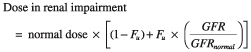Application of the above formula results in the variable dosing strategy shown in Table 4 (where GFR_normal was the ‘normal’ GFR required to clear to enoxaparin without accumulation and defined as 80 ml min⁻¹) [30].

Table 2.

Final parameter estimates from the baseline and covariate model

Baseline Model		Covariate Model
Parameter	Value	SE (CV%)	Value	SE (CV%)
CL (l h−1)	0.536	15.3	renal = 0.681/80 ml min−1	33.3
			non renal = 0.229	49.8
Vc (l)	3.45	17.8	5.22/80 kg (WT)	18.8
Ka (h−1)	0.217	11.6	0.255	16.2
Vp (l)	32.8	23.8	29.6	22.6
Q (l h−1)	0.620	20.2	0.632	21.2
Basal anti-Xa activity (IU l−1)	45.8	32.3	49.9	30.1
ωCL(%CV)	43.1	50.3	32.7	62.3
ωVc (%CV)	61.8	32.5	34.4	72.2
ωQ (%CV)	68.3	37.0	69.8	41.9
ωBasal (%CV)	84.9	29.4	76.6	30.2
Additive error σ1 (IU l−1)	51.1	41.0	52.4	37.5
Proportional error σ2 (%CV)	19.4	36.2	20.0	35.6

Table 3.

Model development

Model	Covariate	OBJ	Δ OBJ	Best model
1	Baseline model	3324.267	–
2	Lean body weight on CL	3322.494	1.77 ns	1
3	Ideal body weight on CL	3319.505	4.76*	2
4	Height on CL	3321.924	2.34 ns	2
5	Sex on CL	3319.935	4.33*	2
6	GFR (using total body weight) on CL	3318.856	5.41*	6
7	GFR (using lean body weight) on CL	3316.755	7.51**	7
8	GFR (using ideal body weight) on CL	3315.121	9.15**	8
9	Total body weight on Vc	3308.023	16.24***	9
10	Lean body weight on Vc	3315.339	8.93**	9
11	Predicted normal weight on Vc	3312.715	11.55***	9
12	Body mass index on Vc	3311.936	12.33***	9
13	Lean body weight on Q	3319.572	4.70*	9
14	Predicted normal weight on Q	3320.331	3.94*	9
15	GFR (using ideal body weight) on CL + total body weight on Vc	3297.990	26.28	15

Δ OBJ = change in OBJ from baseline model.

GFR = glomerular filtration rate, CL = clearance, V_c = central volume of distribution, Q = intercompartmental clearance

^*<0.05

^**<0.01

^***<0.001 based on a χ² distribution.

Figure 1.

Diagnostic plots for baseline and final covariate model. Figure. 1(a,c) are the observed vs. predicted plots for the baseline and final covariate model, respectively. Figure. 1(b,d) are the weighted residual plots for the baseline and final covariate models, respectively

Table 4.

Suggested dosing regimen based on estimated GFR

Estimated GFR* ml min−1	Enoxaparin dose mg kg−1 (WT) twice daily
10–19	0.3
20–29	0.4
30–39	0.5
40–49	0.6
50–59	0.7
60–69	0.8
70–79	0.9
≥80	1

GFR calculated using Cockroft and Gault equation where ideal body weight (IBW) was used as the size descriptor.

Dosing simulations

A number of stochastic simulation experiments were performed using the final covariate model, with the final dosing algorithm (Table 4) suggesting anti-Xa concentrations would be slow to rise, with the therapeutic window of 500–1000 IU l⁻¹ not reached by day 7 (Figure 2). However, if all patients received 1.0 mg kg⁻¹ body weight twice daily regardless of GFR, therapeutic concentrations appear to be achieved within 24 h, but continue to rise in patients with renal impairment. Figure 3 depicts the relationship between the median peak anti-Xa concentration on day 7 plotted against GFR. The curve is relatively flat in patients with a GFR of 50 ml min⁻¹ or above, however, there is progressive accumulation as GFR falls below 50 ml min⁻¹.

Figure 2.

Simulated anti-Xa concentrations for patients with a distribution of renal function recruited in the study using the variable dosing strategy shown in Table 4. The upper, middle and lower lines represent the 90th, 50th and 10th percentiles, respectively

Figure 3.

Simulated peak anti-Xa concentrations at 7 days vs. GFR for patients with a distribution of renal function recruited in the study using the standard dose of 1.0 mg kg⁻¹ body weight. The upper, middle and lower lines represent the 90th, 50th and 10th percentiles, respectively

In view of the clinical necessity to achieve therapeutic anticoagulation quickly, we evaluated a loading dose strategy of 1 mg kg⁻¹ body weight 12 hourly given for three, four, or five doses irrespective of GFR, followed by the variable dosing strategy according to GFR (as per Table 4). Three loading doses resulted in a predicted median trough concentration of 500 IU l⁻¹, although this could not be maintained upon initiation of the variable dosing strategy shown in Table 4 (data not shown). The best compromise between therapeutic dosing and over-anticoagulation was achieved with a four-dose loading strategy as seen in Figure 4. It should be noted that the variable dosing regimen leads to stable anti-Xa concentrations over time, with negligible trends to higher concentrations. Two other simulations were performed which depict the current manufacturer's dosing recommendation in Australia (Figure 5). The first (Figure 5a) shows the profile for administering 1.0 mg kg⁻¹ body weight once daily in patients with an estimated GFR below 30 ml min⁻¹. Whilst this avoids accumulation, the median anti-Xa concentration is predominantly below the target trough concentration of 500 IU l⁻¹ for the first 48 h. The second graph (Figure 5b) shows the profile for 1.0 mg kg⁻¹ twice daily as advised in patients with an estimated GFR of 30 ml min⁻¹ or greater. Therapeutic concentrations are reached quickly, but accumulation continues to occur (which largely reflects accumulation in patients with a GFR of 30–50 ml min⁻¹ as depicted in Figure 3). This is in contrast to our suggested dosing algorithm for this population shown in Figure 4(b).

Figure 4.

Simulated anti-Xa concentrations using a loading dose of 1.0 mg kg⁻¹ total body weight given 12 hourly for 4 doses (2 days) then dose adjusting as shown in Table 4. The upper, middle and lower lines represent the 90th, 50th and 10th percentiles, respectively. Figure 4(a) represents patients with a GFR < 30 ml min⁻¹ and Figure 4(b) represents those patients with a GFR ≥ 30 ml min⁻¹

Figure 5.

Simulated anti-Xa concentrations using the current manufacturer's dosing recommendations (in Australia). The upper, middle and lower lines represent the 90th, 50th and 10th percentiles, respectively. Figure 5(a) represents patients with GFR < 30 ml min⁻¹ given 1.0 mg kg⁻¹ of enoxaparin (total body weight) once daily and Figure 5(b) represents patients with a GFR ≥ 30 ml min⁻¹ given 1.0 mg kg⁻¹ of enoxaparin (total body weight) twice daily

Safety analysis

Four patients experienced minor bleeding, two of which did not require cessation of enoxaparin (haemoptysis 24 h following an episode of acute pulmonary oedema, minor self-limiting epistaxis). Of the other two patients, one developed a haemarthrosis of the right knee (they were also on tirofiban), and the other a groin haematoma related to a cardiac catheter procedure performed after they were no longer in the trial. Observed peak anti-Xa concentrations ranged from 480 to 1130 IU l⁻¹ and troughs 60–760 IU l⁻¹. Three patients received enoxaparin 1.0 mg kg⁻¹ and one received 0.75 mg kg⁻¹. Only one patient experienced a major bleeding complication (retroperitoneal haemorrhage), which required a blood transfusion. The enoxaparin dose was 0.75 mg kg⁻¹; and observed anti-Xa trough concentrations ranged from 290 to 790 IU l⁻¹ (no peaks were recorded). Thrombocytopenia (platelet count <100 000 mm³) was not observed in any of these patients.

Discussion

Enoxaparin is currently the most widely used LMWH for the prevention of recurrent cardiac events in acute coronary syndrome patients. Its clinical utility is based upon simplicity of subcutaneous administration and the perceived nonrequirement for laboratory anticoagulation monitoring. The hydrophilic disposition of LMWHs such as enoxaparin can result in accumulation for those with significant renal impairment, which is not uncommon in patients with acute coronary syndrome. Little information has been presented in the literature that quantifies dosing requirements of enoxaparin in patients with renal impairment. We provide a dosing algorithm that may be applied to patients with renal impairment.

The paucity of information regarding dosing of enoxaparin in renal impairment has prompted re-analysis of large clinical trials, with both the ESSENCE and TIMI 11B trials shown to have excess bleeding complications in the elderly and those with significant renal impairment [12]. However, knowledge is limited as ESSENCE excluded patients with creatinine clearance below 30 ml min⁻¹ and TIMI 11B excluded patients with serum creatinine above 0.176 mmol l⁻¹. A post hoc analysis of TIMI 11A [11] suggested clearance (CL) was reduced by 22% in patients with a GFR below 40 ml min⁻¹, although only 11 of the 445 study patients actually had a GFR below this level, and no dosing guidelines were provided. A prospective study by Collet et al.[31] used 65% of the total enoxaparin dose for patients with a GFR ≤ 0.5 30 ml min⁻¹ [32] and suggested that anti-Xa concentrations were comparable between a patient population that would have been excluded from TIMI 11A (i.e. patients with renal impairment) and those that would have been eligible for TIMI 11A inclusion. No data were provided on the actual anti-Xa sampling times between groups and doses were adjusted at the discretion of the physician to attain concentrations of 500–1000 IU l⁻¹. Whilst the dose recommended by Collet et al.[35] for patients with a GFR < 30 ml min⁻¹ seems well matched to our model (65%vs. 60% of the total dose, respectively), no information was provided about the actual dose adjustments required. Based on our observed and model predicted anti-Xa concentrations it seems likely that initial doses would need to have been significantly increased to reach the 500–1000 IU l⁻¹ target range, somewhat questioning the viability of a blanket 65% proportional dosing strategy for all patients with a GFR < 30 ml min⁻¹.

In addition to these data, a recent population pharmacokinetic study sought to quantify enoxaparin dose requirements using similar methods to those presented here [33]. Unfortunately a random sparse sampling design without informative priors has probably led to model misspecification (i.e. a two compartment model could not be characterized [34]), although clinically this may not be significant. More importantly the authors purport the use of serum creatinine as a dosing scalar in preference to GFR based solely upon a statistical improvement in model fit to the data. We wish to emphasize that renal function cannot be estimated by simply measuring serum creatinine, a phenomenon that is particularly important for the older population. In the setting of a low lean body (muscle) mass, apparently normal concentrations of serum creatinine can mask significant renal impairment, and thus GFR should be estimated by direct measurement of creatinine clearance or use of the Cockroft and Gault formula. It should also be noted that use of ideal body weight (IBW) as opposed to total body weight (WT) in the Cockroft and Gault formula makes GFR estimation more accurate at extremes of body mass [35].

Normal renal function is now defined as a GFR above 80 ml min⁻¹ (US National Kidney Foundation DOQI Clinical Practice Guidelines) [30] and it is evident from our data that enoxaparin renal clearance decreases progressively from this level. Our model predicts that a reduction in enoxaparin dose by 0.1 mg kg⁻¹ body weight for every 10 ml min⁻¹ reduction in GFR for patients with a baseline GFR below 80 ml min⁻¹ will avoid long-term accumulation. However, any dosing adjustment recommendation needs to balance the risk of accumulation with time (and consequent bleeding complications) with the risk of not achieving therapeutic concentrations (and consequent ischaemic complications). This was highlighted in a recent observational study of acute coronary syndrome patients treated with enoxaparin, where reduced anti-Xa concentrations were an independent risk factor for major cardiac events with a threefold increased risk of death and myocardial infarction over patients with anti-Xa concentrations in the therapeutic range [13]. Furthermore, these reduced anti-Xa concentrations were a direct consequence of dosage adjustment by clinicians in an attempt to avoid bleeding complications, which is particularly important as the risk of major recurrent ischaemic events is highest in the first few days of therapy. Our simulations depicted in Figure 4 predict that 48 h standard dosing (1.0 mg kg⁻¹ 12 hourly) followed by an adjusted dose according to GFR (as per the algorithm in Table 4) would achieve therapeutic concentrations quickly, and avoid accumulation. Given that most acute coronary syndrome patients receive less than 7 days of enoxaparin and that accumulation occurs within that time period in patients with a GFR below 50 ml min⁻¹ (see Figure 3), we suggest that the dosing adjustment should be applied to this group. If however, longer term enoxaparin is planned, then we suggest adjusting the dose in all patients with a GFR below 80 ml min⁻¹. Our data suggest that there is no need to adjust the dose in patients when they are first admitted to hospital, which simplifies management, although this strategy is based on the premise that the desirable therapeutic range is well defined a priori. We have not been able to identify any pharmacokinetic–pharmacodynamic models that have quantified the concentration to ischaemic event relationship, and have therefore been guided by the 1 mg kg⁻¹ dosing arm in the TIMI 11A study [27]. Previous work has suggested that maximum concentration is a good predictor for both minor [36] and major bleeding [11] and the impact of unadjusted loading dosing does need to be evaluated prospectively. What does seem clear is that current dosing recommendations for patients with severe renal impairment do not achieve therapeutic anti-Xa concentrations in a timely manner (Figure 5a). Similarly current recommendations for patients with mild to moderate renal impairment appear to result in enoxaparin accumulation (Figure 5b).

We recognize that this is a relatively small study; however, the intensive sampling strategy used ensured the population pharmacokinetic model could be well characterized, and stratification upon GFR allowed for the influence of renal function to be adequately assessed. Clearly, in order to validate our recommendations a randomized prospective study is necessary and we are currently in the planning process of this.

In conclusion, we believe the dosing protocol presented is effective, simple to apply and obviates the need for serum anti-Xa assays in clinical practice. Clearance of enoxaparin was predictably related to GFR estimated using the Cockroft and Gault equation and maintenance doses can be calculated using standard proportional adjustments based upon the estimation that 71% of the drug is excreted unchanged.

References

- 1.Oler A, Whooley MA, Oler J, et al. Adding Heparin to Aspirin Reduces the Incidence of Myocardial Infarction and Death in Patients With Unstable Angina. A meta-analysis. JAMA. 1996;276:811–5. [PubMed] [Google Scholar]
- 2.Harenberg J. Pharmacology of low molecular weight heparins. Semin Thromb Hemost. 1990;16(Suppl):I2–I8. [PubMed] [Google Scholar]
- 3.Boneu B, Caranobe C, Sie P. Pharmacokinetics of heparin and low molecular weight heparin. Baillieres Clin Haematol. 1990;3:531–44. doi: 10.1016/s0950-3536(05)80017-4. [DOI] [PubMed] [Google Scholar]
- 4.Hirsh J, Levine MN. Low molecular weight heparin. Blood. 1992;79:1–17. [PubMed] [Google Scholar]
- 5.Warkentin T, Levine M, Hirsh J, et al. Heparin-induced thrombocytopenia in patients treated with low molecular weight heparin or unfractionated heparin. N Engl J Med. 1995;332:1330–5. doi: 10.1056/NEJM199505183322003. [DOI] [PubMed] [Google Scholar]
- 6.Young E, Wells P, Holloway S, et al. Ex-vivo and in vitro evidence that low molecular weight heparins exhibit less binding to plasma proteins than unfractionated heparin. Thromb Haemost. 1994;71:300–4. [PubMed] [Google Scholar]
- 7.Young E, Cosmi B, Weitz J, et al. Comparison of the non-specific binding of unfractionated heparin and low molecular weight heparin (enoxaparin) to plasma proteins. Thromb Haemost. 1993;70:625–30. [PubMed] [Google Scholar]
- 8.Cohen M, Demers C, Gurfinkel EP, et al. for the Efficacy and Safety of Subcutaneous Enoxaparin in Non-Q-wave Coronary Events Study Group. A comparison of low-molecular-weight heparin with unfractionated heparin for unstable coronary artery disease. N Engl J Med. 1997;337:447–52. doi: 10.1056/NEJM199708143370702. [DOI] [PubMed] [Google Scholar]
- 9.Antman EM, McCabe CH, Gurfinkel EP, et al. Enoxaparin prevents death and cardiac ischaemic events in unstable angina/non-Q-wave myocardial infarction. Results of the Thrombolysis in Myocardial Infarction (TIMI) IIB trial. Circulation. 1999;100:1593–601. doi: 10.1161/01.cir.100.15.1593. [DOI] [PubMed] [Google Scholar]
- 10.Cadroy Y, Pourrat J, Baladre M-F, et al. Delayed elimination of enoxaparine in patients with chronic renal insufficiency. Thromb Res. 1991;63:385–90. doi: 10.1016/0049-3848(91)90141-i. [DOI] [PubMed] [Google Scholar]
- 11.Becker RC, Spencer FA, Gibson M, et al. for the TIMI 11A investigators. Influence of patient characteristics and renal function on factor Xa inhibition pharmacokinetics and pharmacodynamics after enoxaparin administration in non–ST-segment elevation acute coronary syndromes. Am Heart J. 2002;143:753–9. doi: 10.1067/mhj.2002.120774. [DOI] [PubMed] [Google Scholar]
- 12.Spinler SA, Inverso SM, Cohen M, et al. for the ESSENCE & TIMI 11B, Investigators. Safety and efficacy of unfractionated heparin versus enoxaparin in patients who are obese and patients with severe renal impairment: analysis from the ESSENCE and TIMI 11B studies. Am Heart J. 2003;146:33–41. doi: 10.1016/S0002-8703(03)00121-2. [DOI] [PubMed] [Google Scholar]
- 13.Montalescot G, Collet JP, Payot L, et al. Anti-Xa activity relates to outcome in acute coronary syndromes treated with enoxaparin. Circulation. 2003;108:IV–501. doi: 10.1161/01.CIR.0000136830.65073.C7. [DOI] [PubMed] [Google Scholar]
- 14.Cockroft DW, Gault H. Prediction of creatinine clearance from serum creatinine. Nephron. 1976;16:31–41. doi: 10.1159/000180580. [DOI] [PubMed] [Google Scholar]
- 15.Maitre PL, Bührer M, Thomson D, et al. A three-step approach combining Bayesian regression and NONMEM population analysis: application to midazolam. J Pharmacokinet Biopharm. 1991;19:377–84. doi: 10.1007/BF01061662. [DOI] [PubMed] [Google Scholar]
- 16.Mandema JW, Verotta D, Sheiner LB. Building population pharmacokinetic-pharmacodynamic models. I. Models for covariate effects. J Pharmacokinet Biopharm. 1992;20:511–28. doi: 10.1007/BF01061469. [DOI] [PubMed] [Google Scholar]
- 17.Cheymol G. Effects of Obesity on Pharmacokinetics. Clin Pharmacokinet. 2000;39:215–31. doi: 10.2165/00003088-200039030-00004. [DOI] [PubMed] [Google Scholar]
- 18.Green B, Duffull S. Caution when using Lean Body Weight as a size descriptor for obese subjects. Clin Pharmacol Ther. 2002;72:743–4. doi: 10.1067/mcp.2002.129306. [DOI] [PubMed] [Google Scholar]
- 19.Devine B. Case study number 25 gentamicin therapy. DICP. 1974;8:650–5. [Google Scholar]
- 20.New weight standards for men and women. Stat Bul. 1959;40:1–3. [Google Scholar]
- 21.Bauer LA, Edwards WAD, Dellinger EP, et al. Influence of weight on aminoglycoside pharmacokinetics in normal weight and morbidly obese patients. Eur J Clin Pharmacol. 1983;24:643–7. doi: 10.1007/BF00542215. [DOI] [PubMed] [Google Scholar]
- 22.Holford NHG. A size standard for pharmacokinetics. Clin Pharmacokinet. 1996;30:329–32. doi: 10.2165/00003088-199630050-00001. [DOI] [PubMed] [Google Scholar]
- 23.Du Bois D, Du Bois EF. Clinical calorimetry. Tenth paper. A formula to estimate the approximate surface area if height and weight be known. Arch Intern Med. 1916;17:863. [PubMed] [Google Scholar]
- 24.World Health Organization. Geneva: World Health Organization; 1998. Report of a WHO Consultation on obesity: preventing and managing the global epidemic. [PubMed] [Google Scholar]
- 25.Duffull SB, Dooley MJ, Green B, et al. A standard weight descriptor for dose adjustment in the obese patient. Clin Pharmacokinet. doi: 10.2165/00003088-200443150-00007. in press. [DOI] [PubMed] [Google Scholar]
- 26.Beal SL, Sheiner LB. NONMEM User's Guide, Part. I. San Francisco: University of California at San Francisco; 1992. [Google Scholar]
- 27.The Thrombolysis in Myocardial Infarction (TIMI)11A Trial Investigators. Dose-ranging trial of enoxaparin for unstable angina. results of TIMI. J Am Coll Cardiol. 1997;29:1474–82. [PubMed] [Google Scholar]
- 28.Dawes J, Bara L, Billaud E, et al. Relationship between biological activity and concentration of a low molecular weight heparin (PK 10169) and unfractionated heparin after intravenous and subcutaneous administration. Haemostasis. 1986;16:116–22. doi: 10.1159/000215281. [DOI] [PubMed] [Google Scholar]
- 29.Schoemaker RC, Cohen M. Estimating impossible curves using NONMEM. Br J Clin Pharmacol. 1996;42:283–90. doi: 10.1046/j.1365-2125.1996.04231.x. [DOI] [PMC free article] [PubMed] [Google Scholar]
- 30.K/DOQI clinical practice guidelines for chronic kidney disease. evaluation, classification, and stratification. Kidney Disease Outcome Quality Initiative. Am J Kidney Dis. 2002;39(2 Suppl):S1–246. [PubMed] [Google Scholar]
- 31.Collet J, Montalescot G, Fine E, et al. Enoxaparin in Unstable Angina Patients Who Would Have Been Excluded From Randomized Pivotal Trials. J Am Coll Cardiol. 2003;41:8–14. doi: 10.1016/s0735-1097(02)02664-5. [DOI] [PubMed] [Google Scholar]
- 32.Collet JP, Montalescot G, Choussat R, et al. Enoxaparin in unstable angina patients with renal failure. Int J Cardiol. 2001;80:81–2. doi: 10.1016/s0167-5273(01)00455-7. [DOI] [PubMed] [Google Scholar]
- 33.Hulot J, Vantelon C, Urien S, et al. Effect of Renal Function on the Pharmacokinetics of Enoxaparin and Consequences on Dose Adjustment. Ther Drug Moni. 2004;26:305–10t. doi: 10.1097/00007691-200406000-00015. [DOI] [PubMed] [Google Scholar]
- 34.Green B, Duffull SB. Prospective Evaluation of a D-Optimal designed Population Pharmacokinetic Study. J Pharmacokinet Pharmacodyn. 2003;30:145–61. doi: 10.1023/a:1024467714170. [DOI] [PubMed] [Google Scholar]
- 35.Anastasio P, Spitali L, Frangiosa A, et al. Glomerular filtration rate in severely overweight normotensive humans. Am J Kidney Dis. 2000;35:1144–8. doi: 10.1016/s0272-6386(00)70052-7. [DOI] [PubMed] [Google Scholar]
- 36.Green B, Duffull SB. Development of a dosing strategy for enoxaparin in obese patients. Br J Clin Pharmacol. 2003;56:96–103. doi: 10.1046/j.1365-2125.2003.01849.x. [DOI] [PMC free article] [PubMed] [Google Scholar]