Mixture models and exploratory analysis in networks

Abstract

Networks are widely used in the biological, physical, and social sciences as a concise mathematical representation of the topology of systems of interacting components. Understanding the structure of these networks is one of the outstanding challenges in the study of complex systems. Here we describe a general technique for detecting structural features in large-scale network data that works by dividing the nodes of a network into classes such that the members of each class have similar patterns of connection to other nodes. Using the machinery of probabilistic mixture models and the expectation–maximization algorithm, we show that it is possible to detect, without prior knowledge of what we are looking for, a very broad range of types of structure in networks. We give a number of examples demonstrating how the method can be used to shed light on the properties of real-world networks, including social and information networks.

In the last few years, networks have found use in many fields as a powerful tool for representing the structure of complex systems (1–4). Metabolic, protein interaction, and genetic regulatory networks are now heavily studied in biology and medicine, the Internet and the world wide web in computer and information sciences, food webs and other species interaction networks in ecology, and networks of personal or social contacts in epidemiology, sociology, and the management sciences.

The study of networks goes back much further than the current surge of interest in it, but recent work differs fundamentally from earlier studies in the sheer scale of the networks being analyzed. The networks studied 50 years ago by pioneers in the information and social sciences had, typically, a few dozen vertices and were small enough that they could easily be drawn on a piece of paper and perused for interesting features. In the 21st century, on the other hand, networks of thousands or millions of vertices are not unusual and network data on this scale cannot easily be represented in a way that allows quantitative analysis to be conducted by eye. Instead, we have been obliged to turn to topological measures, computer algorithms, and statistics to understand the structure of today's networks. Much of the current research on networks is, in effect, aimed at answering the question “How can we tell what a network looks like, when we can't actually look at it?”

The typical approach to this problem involves defining measures or statistics to quantify network features of interest: centrality indices (5, 6), degree distributions (7–9), clustering coefficients (10), community structure measurements (11, 12), correlation functions (13, 14), and motif counts (15) are all invaluable tools for shedding light on the topology of networks. Our reliance on measures like these, however, has a downside: they require us to know what we are looking for in advance before we can decide what to measure. People measure correlation functions, for instance, because (presumably) they think there may be interesting correlations in a network; they measure degree distributions because they believe the degree distribution may show interesting features. This approach has certainly worked well: many illuminating discoveries have been made this way. However, it raises an uncomfortable question: could there be interesting and relevant structural features of networks that we have failed to find simply because we haven't thought to measure the right thing?

To some extent, this is an issue with the whole of scientific endeavor. In any field, thinking of the right question can demand as much insight as thinking of the answer. However, there are also things we can do to help ourselves. In this paper, we describe a technique that allows us to detect structure in network data while making only rather general assumptions about what that structure is. Methods of this type are referred to by statisticians as “exploratory” data analysis techniques, and we will make use of a number of ideas from the statistical literature in the developments that follow.

We focus on the problem of classifying the vertices of a network into groups such that the members of each group are similar in some sense. This already narrows the types of structure we consider substantially, but leaves a large and useful selection of types still in play. Some of these types have been studied in the past, but the range of possibilities considered here is far larger than that of previous work. For instance, many researchers have examined “community structure” in networks, also called “homophily” or “assortative mixing,” in which vertices divide into groups such that the members of each group are mostly connected to other members of the same group (11, 12). “Disassortative mixing,” in which vertices have most of their connections outside their group, has also been discussed to a lesser extent (16–18). Effective techniques have been developed that can detect structure of both of these types. But, what should we do if we do not know in advance which type to expect or if our network has some other type of structure entirely whose existence we are not even aware of? One can imagine an arbitrary number of other types of division among the vertices of a network, most of which have probably never been considered explicitly in the past. One possibility, for instance, is a network in which, although there is no conventional assortative mixing, there are certain “keystone” vertices and group membership is defined by which particular keystone or set of keystones a vertex is connected to. Another possibility is a network in which there is both assortative and disassortative mixing between members of the same groups, the groups themselves being defined by the fact that their vertices have the same pattern of preferences and aversions, rather than by any overall assortative or disassortative behavior at the group level. And there are certainly many other possibilities. Such complex structures cannot be detected by the standard methods available to us at present and moreover it seems unlikely in many cases that appropriate specialized detection methods will be developed because of the chicken-and-egg nature of the problem: we would have to know the form of the structure in question to develop such a method, but without a detection method, we cannot discover that form in the first place.

Here we propose an approach to the structural analysis of network data that aims to circumvent these issues. It does so by employing a broad and flexible definition of vertex classes, parametrized by an extensive number of variables and hence encompassing an essentially infinite variety of structural types in the limit of large network size. Certainly our definition includes the standard assortative and disassortative structures discussed above and, as we will see, the method we propose will detect those structures when they are present. However, it is also able to detect a wide variety of other structural types and, crucially, does so without requiring us to specify in advance which particular structure we are looking for: the method simultaneously finds the appropriate assignment of vertices to groups and the parameters defining the meaning of those groups, so that upon completion the calculation tells us not only the best way of grouping the vertices but also the definitions of the groups themselves. Our method, which is based on the numerical technique known as the expectation–maximization algorithm, is also fast and simple to implement. We demonstrate the algorithm with applications to a selection of real-world networks and computer-generated test networks.

The Method

The method we describe is based on a mixture model, a standard construct in statistics, although one that has not yet found wide use in studies of networks. The method works well for both directed and undirected networks, but is somewhat simpler in the directed case, so let us start there.

Suppose we have a network of n vertices connected by directed edges, such as a web graph or a food web. The network can be represented mathematically by an adjacency matrix A with elements A_ij = 1 if there is an edge from i to j and 0 otherwise.

Suppose also that the vertices fall into some number c of classes or groups and let us denote by g_i the group to which vertex i belongs. We will assume that these group memberships are unknown to us and that we cannot measure them directly. In the language of statistical inference they are “hidden” or “missing” data. Our goal is to infer them from the observed network structure. (The number of groups c can also be inferred from the data, but for the moment we will treat it as given.) To infer the group memberships we adopt a standard approach for such problems: we propose a flexible (mixture) model for the groups and their properties, then vary the parameters of the model into order to find the best fit to the observed network.

The model we use is a stochastic one that parametrizes the probability of each possible configuration of group assignments and edges as follows. We define θ_ri to be the probability that a (directed) link from a particular vertex in group r connects to vertex i. In the world wide web, for instance, θ_ri would represent the probability that a hyperlink from a web page in group r links to web page i. In effect θ_ri represents the “preferences” of vertices in group r about which other vertices they link to. In our approach it is these preferences that define the groups: a “group” is a set of vertices that all have similar patterns of connection to others.^† [The idea is similar in philosophy to the block models proposed by White and others for the analysis of social networks (19), although the realization and the mathematical techniques used are different.] Note that there is no assumption that the vertices i to which the members of a group link themselves belong to any particular group or groups; they can be in the same group or in different groups or randomly distributed over the entire network. Thus, the structures we envisage can be quite different from traditional assortatively mixed networks, although they include the latter as a special case.

We also define π_r be the (currently unknown) fraction of vertices in group or class r, or equivalently the probability that a randomly chosen vertex falls in r. The parameters π_r, θ_ri satisfy the normalization conditions

The quantities in our theory thus fall into three classes: measured data {A_ij}, missing data {g_i}, and model parameters {π_r, θ_ri}. To simplify the notation we will henceforth denote by A the entire set {A_ij} and similarly for {g_i}, {π_r}, and {θ_ri}.

The standard framework for fitting models like this one to a given data set is likelihood maximization, in which one maximizes with respect to the model parameters the probability that the data were generated by the given model. Maximum likelihood methods have occasionally been used in network calculations in the past (20–22), as well as in many other problems in the study of complex systems more generally. In the present case, our fitting problem requires us to maximize the likelihood Pr(A, g|π, θ) with respect to π and θ, which can be done by writing

where

so that the likelihood is

In fact, one commonly works not with the likelihood itself but with its logarithm:

The maximum of the two functions is in the same place, because the logarithm is a monotonically increasing function.

Unfortunately, g is unknown in our case, which means the value of the log-likelihood is also unknown. We can, however, usually make a good guess at the value of g given the network structure A and the model parameters π, θ. More specifically, we can, as shown below, calculate the probability distribution Pr(g|A, π, θ) and from it calculate an expected value ℒ̄ for the log-likelihood by averaging over g, thus:

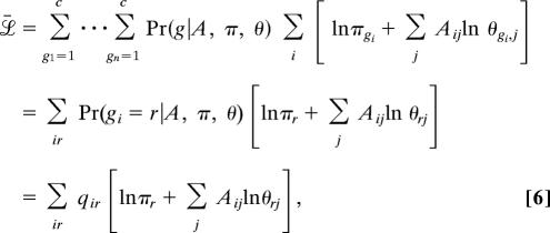where to simplify the notation we have defined q_ir = Pr(g_i = r|A, π, θ), which is the probability that vertex i is a member of group r. (In fact, it is precisely these probabilities that will be the principal output of our calculation.)

This expected log-likelihood represents our best estimate of the value of ℒ and the position of its maximum represents our best estimate of the most likely values of the model parameters. Finding the maximum still presents a problem, however, because the calculation of q requires the values of π and θ and the calculation of π and θ requires q. The solution is to adopt an iterative, self-consistent approach that evaluates both simultaneously. This type of approach, known as an expectation–maximization or EM algorithm, is common in the literature on missing data problems. In its modern form, it is usually attributed to Dempster et al. (23), who built on theoretical foundations laid previously by a number of other authors (24).

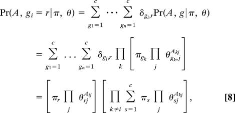
Following the conventional development of the method, we calculate the expected probabilities q of the group memberships given π, θ and the observed data thus:

The factors on the right are given by summing over the possible values of g in Eq. 4 thus:

and

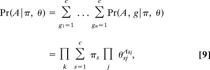where δ_ij is the Kronecker δ symbol. Substituting into Eq. 7, we then find

Note that q_ir correctly satisfies the normalization condition Σ_r q_ir = 1.

Once we have the values of the q_ir, we can use them to evaluate the expected log-likelihood (Eq. 6) and hence to find the values of π,θ that maximize it. One advantage of the current approach now becomes clear: because the q_ir are known, fixed quantities, the maximization can be carried out purely analytically, obviating the need for numerical techniques such as Markov chain Monte Carlo. Introducing Lagrange multipliers to enforce the normalization conditions (Eq. 1) and differentiating, we find that the maximum of the likelihood occurs when

where Σ_j A_ij is the out-degree of vertex i and we have explicitly evaluated the Lagrange multipliers using the normalization conditions.

Eqs. 10 and 11 define our expectation–maximization algorithm. Implementation of the algorithm consists merely of iterating these equations to convergence and the output is the probability q_ir for each vertex to belong to each group, plus the probabilities θ_ri of links from vertices in each group to every other vertex, the latter effectively giving the definitions of the groups. The calculation converges rapidly in practice: typical run times for the networks studied here were fractions of a second. [Some theoretical results are known for the convergence of EM algorithms, see Dempster et al. (23) and Wu (25).]

The obvious choice of starting values for the iteration is the symmetric choice π_i = 1/c, θ_ri = 1/n, but unfortunately these values are a trivial (unstable) fixed point of Eqs. 10 and 11 and hence a poor choice. In our calculations we have instead used starting values that are perturbed randomly a small distance from this fixed point. A random starting condition also gives us an opportunity to assess the robustness of our results. Except in special cases (such as the trivial fixed point above), expectation–maximization algorithms are known to converge to local maxima of the likelihood (24) but not always to global maxima, and hence it is possible to get different solutions from different starting points. The method works well in cases where it frequently converges to the global maximum or where it converges to local maxima that are close to the global maximum, giving good if not perfect solutions on most runs. In practice, we find for some networks that the method almost always converges to the same solution or a very similar one, whereas for others it is necessary to perform several runs with different initial conditions to find a good maximum of the likelihood. In the calculations presented in this paper, we have in each case taken the division of the network giving the highest likelihood over the runs performed.

The developments so far apply to the case of a directed network. Most of the networks studied in the recent literature, however, are undirected. The model used above is inappropriate for the undirected case because its edges represent an inherently asymmetric, directed relationship between vertices in which one vertex chooses unilaterally to link to another, the receiving vertex having no say in the matter. The edges in an undirected network, by contrast, usually represent symmetric relationships. In a social network of friendships, for instance, the edges would typically be drawn undirected because two people can become friends only if both choose to be friendly toward the other. To extend our method to undirected networks, we need to incorporate this symmetry into our model, which we do as follows. Once again, we define θ_ri to be the probability that a vertex in group r “chooses” to link to vertex i, but we now specify that a link will be formed only if two vertices both choose each other. Thus, the probability that an edge falls between vertices i and j, given that i is in group s and j is in group r, is θ_riθ_sj, which is now symmetric. This probability satisfies the normalization condition Σ_ij θ_riθ_sj = 1 for all r,s and setting r = s, we find

and hence Σ_i θ_ri = 1 as before.

Now the probability Pr(A|g, π, θ) in Eq. 4 is given by

exactly as in the directed case, where we have made use of the fact that A_ji = A_ij for an undirected network. (We have also assumed there are no self-edges in the network, edges that connect a vertex to itself, so that A_ii = 0 for all i.)

The remainder of the derivation now follows as before and results in the same equations, 10 and 11, for the final algorithm.

Example Applications

For our first examples of the operation of our method, we apply it to two small networks, one known to have conventional assortative community structure, the other known to have disassortative structure. The first is the much-discussed “karate club” network of friendships between 34 members of a karate club at a U.S. university, assembled by Zachary (26) by direct observation of the club's members. This network is of particular interest because the club split in two during the course of Zachary's observations as a result of an internal dispute, and Zachary recorded the membership of the two factions after the split.

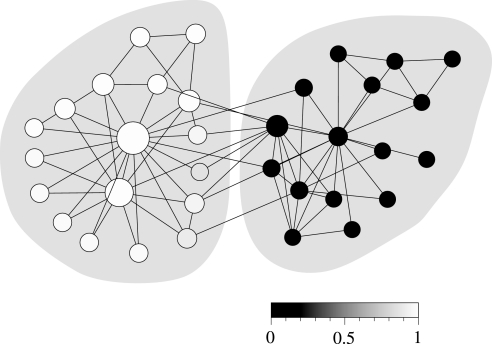
Fig. 1 shows the best division of this network into two groups found using the expectation–maximization method with c set equal to 2. The shades of the vertices in the figure represent the values of the variables q_i1 for each vertex on the scale shown (or equivalently the values of q_i2, because q_i1+q_i2 = 1 for all i). As we can see, the algorithm assigns most of the vertices strongly to one group or the other; in fact, all but 13 vertices are assigned 100% to one of the groups (black and white vertices in the figure). Thus, the algorithm finds a strong split into two clusters in this case, and indeed if one simply divides the vertices according to the cluster to which each is most strongly assigned, the result corresponds perfectly to the division observed in real life (denoted by the shaded regions in the figure).

Fig. 1.

Application of the method described here to the “karate club” network of ref. 26. The two shaded regions indicate the division of the network in the real world, whereas the shades of the individual vertices indicate the decomposition chosen by the algorithm. The sizes of the vertices indicate the probabilities θ_1i for edges from vertices in group 1 (the left group) to be connected to each other vertex, with the probabilities ranging from 0 for the smallest vertices to 0.19 for the largest.

However, the algorithm reveals much more about the network than this. First, where appropriate it can return probabilities for assignment to the two groups that are not 0 or 1 but lie somewhere between these limits, and for some of the vertices in this network it does so. Inspection of the figure reveals in particular a small number of vertices with intermediate shades of gray along the border between the groups. There has been some discussion in the recent literature of methods for divining “fuzzy” or overlapping groups in networks; rather than dividing a network sharply into groups, it is sometimes desirable to assign vertices to more than one group and a number of possible ways of doing this have been proposed (17, 27–29). The present algorithm offers an alternative method that is particularly attractive because of the clear definition of the overlap: the values of the q_ir give the precise probability that a vertex belongs to a specified group, given the observed network structure.

The algorithm also returns the distributions or preferences θ_ri for connections from vertices in group r to each other vertex i. In Fig. 1, we indicate by the sizes of vertices the probabilities θ_1i of edges from vertices in group 1, which is the left group in Fig. 1, to connect to each other vertex. As we can see, two vertices central to the group have high connection probabilities, whereas some of the more peripheral vertices have smaller probabilities. Thus, the values of θ_ri behave as a kind of centrality measure, indicating how important a particular vertex is to a particular group. This could form the basis for a practical measure of within-group influence or attraction in social or other networks. Note that, in this case, this measure is not high for vertices that are central to the other group, group 2; the measure is sensitive to the particular preferences of the vertices in just a single group.

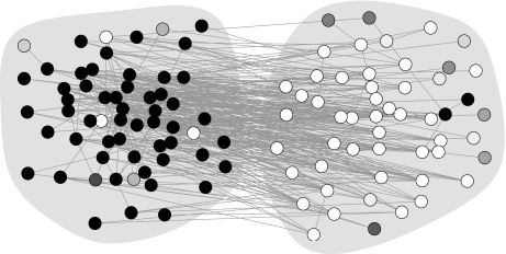
We can take the method further. In Fig. 2, we show the results of its application to an adjacency network of English words taken from ref. 17. In this network, the vertices represent 112 commonly occurring adjectives and nouns in a particular body of text (the novel David Copperfield by Charles Dickens), with edges connecting any pair of words that appear adjacent to each other at any point in the text. Because adjectives typically occur next to nouns in English, most edges connect an adjective to a noun and the network is thus approximately bipartite or disassortative. This can be seen clearly in Fig. 2, where the two shaded groups represent the adjectives and nouns and most edges are observed to run between groups.

Fig. 2.

The adjacency network of English words described in the text. The two shaded groups contain adjectives and nouns respectively and the shades of the individual vertices represent the classification found by the algorithm.

Analyzing this network using our algorithm we find the classification shown by the shades of the vertices. Once again, most vertices are assigned 100% to one class or the other, although there are a few ambiguous cases, visible as the intermediate shades. As Fig. 2 makes clear, the algorithm's classification corresponds closely to the adjective/noun division of the words, almost all of the black vertices falling in one group and the white ones in the other. In fact, 89% of the vertices are correctly classified by our algorithm in this case.

The crucial point to notice, however, is that the algorithm is not merely able to detect the bipartite structure in this network, but it is able to do so without being told that it is to look for bipartite structure. The exact same algorithm, unmodified, finds both the assortative structure of Fig. 1 and the disassortative structure of Fig. 2. This is an important strength of the present method: it is able to detect a range of different structural types without knowing in advance what type to expect. Other methods are able to detect particular kinds of structure, and in many cases do a good job, but they tend to be narrowly tailored to that job. Typically a new method or algorithm has to be devised for each new structural type.

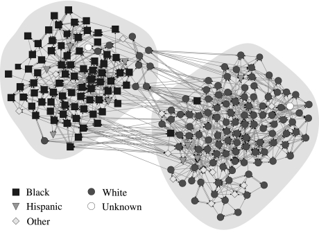
The networks in Figs. 1 and 2 are both undirected, but our method is applicable to directed networks as well. In Fig. 3, we show an example of a directed network, a social network of high school students taken from the U.S. National Longitudinal Study of Adolescent Health (the “AddHealth” study). Students were asked to identify their friends within the school and a response in which student A identifies B as a friend is represented as a directed edge from A to B. In contrast to the common view, discussed earlier, of friendship as a symmetric relationship running in both directions between the individuals it connects, a remarkable number of the friendships identified in this study, more than half, are found to run in only one direction, so that a directed representation of the network is indispensable for capturing the structure of the data.

Fig. 3.

A directed social network of U.S. high school students and the division into two groups found by the directed version of our method. Vertex shapes show the (self-identified) ethnicity of the students, as indicated.

Applying the directed version of our method to this network with c = 2 produces the division shown in Fig. 3. This example is striking because, like many of the networks in the AddHealth data set, the groupings are found to correlate strongly with student ethnicity as shown by the shapes of the vertices (30). In this case, one of the two groups contains most of the school's black students and the other most of the white students, with the few members of other ethnic groups distributed more evenly.

The examples we have seen so far all center on networks with strong assortative or disassortative mixing, but it is important to emphasize that our method is applicable to other types of structure as well. For our final example, we focus on a network of a completely different kind, a computer-generated network of a form mentioned in the introduction. In this network there are a small number of “keystone” vertices and group membership affects only the propensity to link to these vertices; all other connections are purely random. In detail, the network is as follows.

The network is again a directed one, with a total of 108 vertices. One hundred of those vertices are divided into four groups of 25 each, and directed edges are placed uniformly at random between them such that the mean degree (both in and out) is 10. The remaining eight vertices are denoted keystone vertices and the other vertices link to them depending on their group membership. Specifically, the vertices in groups A, B, C, and D link to keystone vertices {1,2,3,4}, {3,4,5,6}, {5,6,7,8}, and {7,8,1,2}, respectively. Thus, no keystone vertex is uniquely identified with any group, but each group has a unique signature set of keystones, and it is only this pattern of keystone links that distinguishes the group. The network is not assortative (or disassortative) by the traditional definition: the randomly placed edges fall within or between groups purely according to chance, and the links to the keystones, although not random, are equally likely to fall within or between groups.

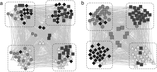
Fig. 4a shows what happens when we analyze this network using a standard community detection technique. The dashed boxes in the figure outline the four groups of vertices and the shapes show the group assignments found by the analysis. Although the analysis does find four groups in this case, the groups do not correspond to the known division of the network: each box contains substantial numbers of vertices of at least two types and in some cases more. The maximum likelihood analysis, by contrast, has no difficulty in discerning the structure of the network. Fig. 4b shows the output of our algorithm with c = 4 and, as we can see, the algorithm has, without prior knowledge of the type of structure in the network, discovered the structure and correctly assigned almost all of the vertices to their groups. The eight keystone vertices, which are shown in the center of Fig. 4b, are not assigned to any group by the algorithm, but are instead divided (almost) equally between all four (meaning that q_ir is close to 0.25 for all r). Thus, the algorithm has, in effect, accurately deduced the five classes of vertices present in the network. Moreover, an examination of the final values of the model parameters θ_ri will tell us exactly what type of structure the algorithm has discovered. In principle, considerably more complex structures than this can be detected as well.

Fig. 4.

The four-group network described in the text, in which connections between vertices are entirely random, except for connections to the eight keystone vertices in the center. Each of the four groups (dashed boxes) is thus distinguished solely by the unique pattern of its connections to the keystone vertices. Vertex shapes represent the groups to which vertices are assigned by our analyses using the traditional community detection (a) and maximum likelihood (b) methods of this paper.

Conclusions

In this paper, we have described a method for exploratory analysis of network data in which vertices are classified into groups based on the observed patterns of connections between them. The method is more general than previous clustering methods, making use of maximum likelihood techniques to classify vertices and simultaneously determine the definitive properties of each class. The result is a simple algorithm that is capable of detecting a broad range of structural signatures in networks, including conventional community structure, bipartite or disassortative structure, fuzzy, or overlapping classifications, and many mixed or hybrid structural forms that have not been considered explicitly in the past. We have demonstrated the method with applications to a variety of examples, including real-world and computer-generated networks. The method's strength is its flexibility, which will allow researchers to probe observed networks for general types of structure without having to specify in advance what type they expect to find.

References

- 1.Newman MEJ, Barabási A-L, Watts DJ. The Structure and Dynamics of Networks. Princeton: Princeton Univ Press; 2006. [Google Scholar]
- 2.Albert R, Barabási A-L. Rev Mod Phys. 2002;74:47–97. [Google Scholar]
- 3.Newman MEJ. SIAM Rev. 2003;45:167–256. [Google Scholar]
- 4.Boccaletti S, Latora V, Moreno Y, Chavez M, Hwang D-U. Phys Rep. 2006;424:175–308. [Google Scholar]
- 5.Wasserman S, Faust K. Social Network Analysis. Cambridge, UK: Cambridge Univ Press; 1994. [Google Scholar]
- 6.Scott J. Social Network Analysis: A Handbook. 2nd Ed. London: Sage; 2000. [Google Scholar]
- 7.Albert R, Jeong H, Barabási A-L. Nature. 1999;401:130–131. [Google Scholar]
- 8.Faloutsos M, Faloutsos P, Faloutsos C. Comput Comm Rev. 1999;29:251–262. [Google Scholar]
- 9.Kleinberg JM, Kumar SR, Raghavan P, Rajagopalan S, Tomkins A. In: Asano T, Imai H, Lee DT, Nakano S-I, Tokuyama T, editors. Proceedings of the 5th Annual International Conference on Combinatorics and Computing; Berlin: Springer; 1999. pp. 1–18. Lecture Notes in Computer Science. [Google Scholar]
- 10.Watts DJ, Strogatz SH. Nature. 1998;393:440–442. doi: 10.1038/30918. [DOI] [PubMed] [Google Scholar]
- 11.Girvan M, Newman MEJ. Proc Natl Acad Sci USA. 2002;99:7821–7826. doi: 10.1073/pnas.122653799. [DOI] [PMC free article] [PubMed] [Google Scholar]
- 12.Danon L, Duch J, Diaz-Guilera A, Arenas A. J Stat Mech. 2005 P09008. [Google Scholar]
- 13.Pastor-Satorras R, Vázquez A, Vespignani A. Phys Rev Lett. 2001;87:258701. doi: 10.1103/PhysRevLett.87.258701. [DOI] [PubMed] [Google Scholar]
- 14.Newman MEJ. Phys Rev Lett. 2002;89:208701. doi: 10.1103/PhysRevLett.89.208701. [DOI] [PubMed] [Google Scholar]
- 15.Milo R, Shen-Orr S, Itzkovitz S, Kashtan N, Chklovskii D, Alon U. Science. 2002;298:824–827. doi: 10.1126/science.298.5594.824. [DOI] [PubMed] [Google Scholar]
- 16.Holme P, Liljeros F, Edling CR, Kim BJ. Phys Rev E. 2003;68 doi: 10.1103/PhysRevE.68.056107. 056107. [DOI] [PubMed] [Google Scholar]
- 17.Newman MEJ. Phys Rev E. 2006;74 036104. [Google Scholar]
- 18.Estrada E, Rodríguez-Velázquez JA. Phys Rev E. 2005;72 doi: 10.1103/PhysRevE.72.046105. 046105. [DOI] [PubMed] [Google Scholar]
- 19.White HC, Boorman SA, Breiger RL. Am J Sociol. 1976;81:730–779. [Google Scholar]
- 20.Jones JH, Handcock MS. Proc R Soc London B. 2003;270:1123–1128. doi: 10.1098/rspb.2003.2369. [DOI] [PMC free article] [PubMed] [Google Scholar]
- 21.Clauset A, Newman MEJ, Moore C. Proceedings of the 23rd International Conference on Machine Learning; New York: Assoc Comp Machinery; 2006. [Google Scholar]
- 22.Hastings MB. Phys Rev E. 2006;74 035102. [Google Scholar]
- 23.Dempster AP, Laird NM, Rubin DB. J R Statist Soc B. 1977;39:185–197. [Google Scholar]
- 24.McLachlan GJ, Krishnan T. The EM Algorithm and Extensions. New York: Wiley; 1996. [Google Scholar]
- 25.Wu CFJ. Ann Stat. 1983;11:93–103. [Google Scholar]
- 26.Zachary WW. J Anthropol Res. 1977;33:452–473. [Google Scholar]
- 27.Reichardt J, Bornholdt S. Phys Rev Lett. 2004;93:218701. doi: 10.1103/PhysRevLett.93.218701. [DOI] [PubMed] [Google Scholar]
- 28.Palla G, Derényi I, Farkas I, Vicsek T. Nature. 2005;435:814–818. doi: 10.1038/nature03607. [DOI] [PubMed] [Google Scholar]
- 29.Baumes J, Goldberg M, Magdon-Ismail M. Proceedings of the IEEE International Conference on Intelligence and Security Informatics; New York: Institute of Electrical and Electronics Engineers; 2005. [Google Scholar]
- 30.Moody J. Am J Sociol. 2001;107:679–716. [Google Scholar]
Associated Data
This section collects any data citations, data availability statements, or supplementary materials included in this article.