

Abstract
Virtual microscopy involves the conversion of histological sections mounted on glass microscope slides to high resolution digital images. Virtual microscopy offers several advantages over traditional microscopy, including remote viewing and data-sharing, annotation, and various forms of data-mining.
We describe a method utilizing virtual microscopy for generation of internet-enabled, high-resolution brain maps and atlases. Virtual microscopy-based digital brain atlases have resolutions approaching 100,000 dpi, which exceeds by three or more orders of magnitude resolutions obtainable in conventional print atlases, MRI, and flat-bed scanning. Virtual microscopy-based digital brain atlases are superior to conventional print atlases in five respects: 1) resolution, 2) annotation, 3) interaction, 4) data integration, and 5) data-mining.
Implementation of virtual microscopy-based digital brain atlases is located at BrainMaps.org, which is based on more than 10 million megapixels (35 terabytes) of scanned images of serial sections of primate and non-primate brains with a resolution of 0.46 microns/pixel (55,000 dpi).
The method can be replicated by labs seeking to increase accessibility and sharing of neuroanatomical data. Online tools offer the possibility of visualizing and exploring completely digitized sections of brains at a sub-neuronal level, and can facilitate large-scale connectional tracing, histochemical and stereological analyses.
1 Introduction
Internet technologies have revolutionized the way we access and share data (Martone, Gupta, & Ellisman, 2004). In recent years, the merging of internet and digital technologies with conventional microscopy has created revolutionary new capabilities for online viewing and navigation through high-resolution digitized “virtual” slides (Ferreira, Moon, Humphries, Sussman, Saltz, Miller, & Demarzo, 1997; Afework, 1998; Felten, Strauss, Okada, & Marchevsky, 1999; Romer & Suster, 2003). These new digital capabilities are commonly referred to as “virtual microscopy”.
Virtual slides facilitate data sharing by transmission over computer networks and offer considerable advantages over conventional glass microscope slides in terms of ease and speed of navigation and inspection of large numbers of brain sections. Virtual slides also facilitate visualization and neuroanatomical analysis. With current scanners, it is possible to achieve resolutions of digitized slides at more than 100,000 dpi, enabling the creation of brain atlases at microscopic resolution that far exceeds the resolutions obtainable through the use of other digital scanning technologies, MRI, or in conventional print media. The immense size of high-resolution neuroanatomical image datasets, however, presents an obstacle to visualization, manipulation, and analysis, especially when used online.
At BrainMaps.org, we have created a zoomable high-resolution digital brain atlas and virtual microscope that is based on more than 10 million megapixels of scanned images of serial sections of primate and non-primate brains. In this technical resport, we describe how the atlas has been created, how it is integrated with a high-speed database for querying and retrieving data about brain structure and function over the internet, and describe how readily available software tools can be applied in visualization of the high resolution images.
The resolution of the images, 0.46 micron per pixel, is considerably higher than any histological atlases currently available, either in print or in digital form, and is approximately three orders of magnitude greater than the resolution of MRI acquired brain images. The atlas permits a viewer to zoom in from the gross sectional outline to the sub-neuronal level, exactly as if viewing the sections through a microscope.
2 Materials and Methods
Figure 1 outlines the major steps in going from stained or immunocytochemically or histochemically processed slide-mounted sections of brains to a web-accessible image pyramid. Each of the individual steps is considered below.
Figure 1.
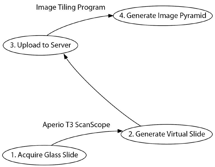
High-throughput virtual microscopy. Block diagram outlining the major steps in going from immunocytochemically or histochemically processed slide-mounted tissue to a web-accessible image pyramid.
2.1 Acquisition of Glass Slide Datasets
Various datasets were available, made up of serial sections of brains stained by the Nissl stain or by histochemistry or immunocytochemistry. Species included were Macaca mulatta, Macaca fascicularis, Chlorocebus aethiops, Homo sapiens, Felis catus, Mus musculus, and Tyto alba (Table 1). Brains were sectioned frozen or after embedding in celloidin in the frontal, horizontal, or sagittal planes. Three of the Macaca mulatta brains contained fiduciary marks made by inserting electrodes at fixed stereotaxic coordinates prior to perfusion with fixative.
Table 1.
Datasets from various species utilized in this study.
| Species | Datasets | Sections |
|---|---|---|
| Homo sapiens | 6 | 163 |
| Macaca mulatta | 15 | 703 |
| Macaca fascicularis | 1 | 6 |
| Chlorocebus aethiops | 1 | 740 |
| Felis catus | 9 | 195 |
| Mus musculus | 13 | 994 |
| Tyto alba | 4 | 182 |
2.2 Generating Virtual Slides
Glass-mounted sections were scanned at 20x (0.46 um/pixel) in an Aperio ScanScope T3 scanner (Aperio Technologies, Vista, CA, USA), specially adapted to accommodate 3”×2” slides, to generate virtual slides. The 3”×2” slide size limitation prevents larger sections such as whole human brain slices from being scanned in toto, which would require at least an 8”×6” slide size. Montaging is one way around the slide size limitation, though it was not employed in this study. Thus, our human brain virtual slide data consists of sections from smaller blocks of brain such as the diencephalon. The image file format used for the virtual slides is JPEG-compressed TIFF, which results in 1/15 compression ratio (and corresponding reduction in file size) with no perceptible loss of image quality. The raw size of each virtual slide is typically about 25 gigabytes uncompressed, but as a JPEG-compressed TIFF, is reduced to 1.5 to 2.5 gigabytes.
Since the width of each virtual slide commonly exceeds 100,000 pixels, the slides cannot be saved solely as JPEG since JPEG files cannot exceed 30,000 pixels in either width or height. The TIFF file format has a maximum size of 4 gigabytes, making the use of TIFF alone not an option for images greater than this maximum. However, as JPEG-compressed TIFFs, it is possible to save 25 gigabyte images of 100,000 pixel width, thereby making JPEG-compressed TIFF currently the sole option for use with the very large images used in constructing the database. The compression schemes offered by DJVU and JPEG2000 present alternatives to JPEG but were not employed due to incompatibility with tiling software used to generate image pyramids. Other “lossless” file formats, such as PNG, are not practicable at this stage due to the excessive disk space that would be consumed (commonly exceeding 25 gigabytes per image).
JPEG compression, although it has been designed with the goal to compress images in a manner that loss of information is not perceptible by the eye, is still not entirely “loss-less” and may be problematic for certain types of image processing algorithms, such as image derivatives used in automated analysis, or in various datamining applications used in automatic analysis.
2.3 Generating Image Pyramids
Following virtual slide generation, virtual slides are uploaded to the image hard drives on the server, via File Transfer Protocol (FTP) or other network protocols.
In the final step, virtual slides are converted to a digital format that permits rapid web-based navigation and visualization using software customized for working with very large images; tiled to multiple small (256×256 pixels) JPEG images to generate composite hierarchically-organized, multiresolution image pyramids (Figure 2), and are finally integrated into a relational database.
Figure 2.
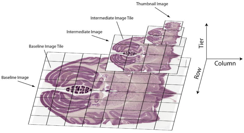
The concept behind an image pyramid. Each virtual slide, representing a single monolithic image file, is chopped up (i.e., tiled) to generate a multi-resolution image pyramid composed of small image tiles with a maximum size of 256 × 256 pixels. Image pyramids allow for rapid online navigation through very large images by loading only the image tiles that are currently being viewed.
Strictly speaking, the image pyramid is still considered a “virtual slide”, although it consists of multiple files (image tiles) instead of a monolithic image file.
Image Tile Generation, Placement, and Retrieval
The Zoomifier EZ tool (Zoomify Inc., Santa Cruz, CA, USA) is used to produce the tiled image pyramid. It generates the image tiles at multiple resolutions (each resolution differs from the preceding one by a multiple of two), places them into a canonical directory, and writes an information file (ImageProperties.xml) at the top of the directory. The meaning of the terms used in ImageProperties.xml are shown in Table 2, along with the terms used in this paper.
Table 2.
Terms used in ImageProperties.xml.
| Constant | This paper | Meaning |
|---|---|---|
| TILESIZE | T | Dimensions of square image tile in pixels |
| WIDTH | W | Width of full-sized image in pixels |
| HEIGHT | H | Height of full-sized image in pixels |
| NUMTILES | N | Total number of all images tiles in this image pyramid |
The first column is the variable as shown in the file, the second column is the term used in this paper, and the third column describes the meaning of the term.
Image tiles are named using the pattern http://baseName/TileGroupG/T-C-R.jpg in which baseName represents the path to the directory containing ImageProperties.xml, G is an integer such that 0 ≤ G ≤ dN/256e, T is the tier number of the desired image such that 0 ≤ T ≤ ⌈log2(max(W,H)/T)⌉, and C and R are the column and row (each numbered from 0) of the tile in the image at tier T.
The data in ImageProperties.xml, along with the knowledge of data file placement, are key to retrieving the image tiles necessary to reconstruct the desired image. It is also helpful to know that logically the tile image files are created and stored in row-order starting with Tier 0 in TileGroup0, and that each TileGroup directory is completely filled with 256 entries before another is started. A detailed example of image tile retrieval can be found in Appendix 5.
2.4 Total Quantity of Virtual Slides
A total of 3035 sections of primate and nonprimate brains were scanned at 0.46 microns per pixel, digitized, and uploaded to the server at BrainMaps.org. The total quantity of image data currently directly accessible online is 10,569,936 MegaPixels (or 31.71 TeraBytes, uncompressed) (Figure 3).
Figure 3.
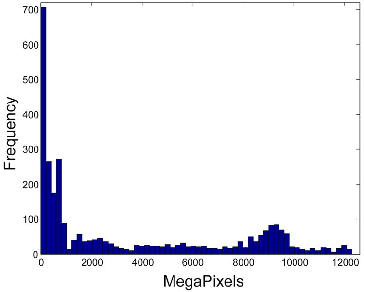
Distribution of image sizes at BrainMaps.org as of 09-25-2006. The total size of the brain images is 10,569,936 MegaPixels, or 31.71 TeraBytes. The total number of images is 3035, with an average size of 3482.68 MegaPixels/image (or 10.45 GigaBytes/image).
2.5 Server Architecture
The server architecture (Figure 4) can be divided into four main components: 1) the web server (Microsoft IIS), 2) the relational database management system (MySQL), 3) the internal hard disk drives, denoted HDD (PHP), for holding web server PHP scripts and MySQL database files, and 4) the external image data hard disk drives, labeled HDD (1) and HDD (2), for holding image data (LaCie, 2TB LaCie Biggest, RAID 5). The first three components are straight-forward to implement and require no additional explanation except to note that the first component, the IIS web server, utilizes the PHP active scripting language to dynamically generate HTML and embed the graphical user interface. Regarding the fourth component, multiple external image data HDD’s can be added as additional image data is added to the server. Each LaCie (LaCie USA, Hillsboro, OR, USA) external HDD disk array holds 2 terabytes. The external HDDs are configured as a RAID 5 array, which has redundancy spread over disks so that, in the event of hard disk failure, no data will be lost. Buffalo Technology (Buffalo Technology Inc, Austin, TX, USA) produces a similar 2 terabyte, RAID 5 disk storage system.
Figure 4.
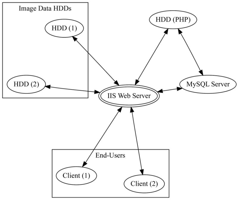
Server organization. The client interacts with the server through a Flash or Java based frontend that interacts with the image file system and relational database. The active scripting language, PHP, is used as a ‘glue’ to tie all the components together.
2.6 Online Navigation and Graphical User Interfaces
Clients interact with the web server (Figure 4) to access image data or retrieve database information. Clients can access the image data either through a web browser (Client A in Figure 4) or a different desktop application (Client B in Figure 4). If accessed through a web browser, then the graphical user interface (GUI) to the image data is coded through Flash, AJAX, or Java. If accessed through a different desktop application, then the GUI can be written in other programming languages, such as C.
We have coded GUI’s for the brainmaps.org image data in Flash, Java, and C. The brainmaps.org GUI can also be coded in AJAX. Each programming language has its own strengths and weaknesses for the GUI. For example, Java is relatively slow for a GUI and requires a separate browser plugin, but it has the advantage of more sophisticated programming. The C programming language is fast and versatile but is operating system-dependent and driver-dependent. Flash is fast but requires a browser plugin (which, however, is present on over 90% of browsers). AJAX is fast, but may have browser compatibility issues and requires that Javascript be enabled (about 10% of users disable Javascript).
Figure 5 shows an example of navigation through virtual slides using the Chlorocebus aethiops Nissl dataset. All images are screenshots from a web browser and are what a visitor to brainmaps.org sees: (a) An array of virtual slides for the Chlorocebus aethiops dataset, shown as clickable thumbnails that, when clicked on, launch a new browser window allowing navigation through the high-resolution image (b). The image in (b) is 95,040 × 74,711 pixels and 20 gigabytes in size. The thumbnail in the upper left is for navigation purposes. Shown also are overlying labels of brain areas that can be toggled on and off. (c) Zooming in on the slide in (b). The red box in (b) corresponds to (c). (d) Zooming in to full resolution in (c), showing details of individual neurons in the insular cortex. The red box in (c) corresponds to (d).
Figure 5.

An example of navigation through virtual slides at brainmaps.org using the African green monkey Nissl dataset. All images are actual screenshots from a web browser and are what a visitor to brainmaps.org would see. (a) An array of virtual slides for the dataset, shown as clickable thumbnails that, when clicked on, launch a new browser window allowing navigation through the high-resolution image (b). The image in (b) is 95,040 × 74,711 pixels and 20 gigabytes in size. The thumbnail in the upper left is for navigation purposes. Shown also are overlying labels of brain areas that may be toggled on and off. (c) Zooming in on the slide in (b). The red box in (b) corresponds to (c). (d) Zooming in to full resolution in (c), showing details of individual neurons in the insula. The red box in (c) corresponds to (d).
Figure 6 shows an example of a Flash-based GUI for viewing the high-resolution images. The label-specific context menu in the upper right enables the user to retrieve related information, including the position of the label in the labeling hierarchy, connectivity, and gene expression patterns derived from other slide datasets.
Figure 6.
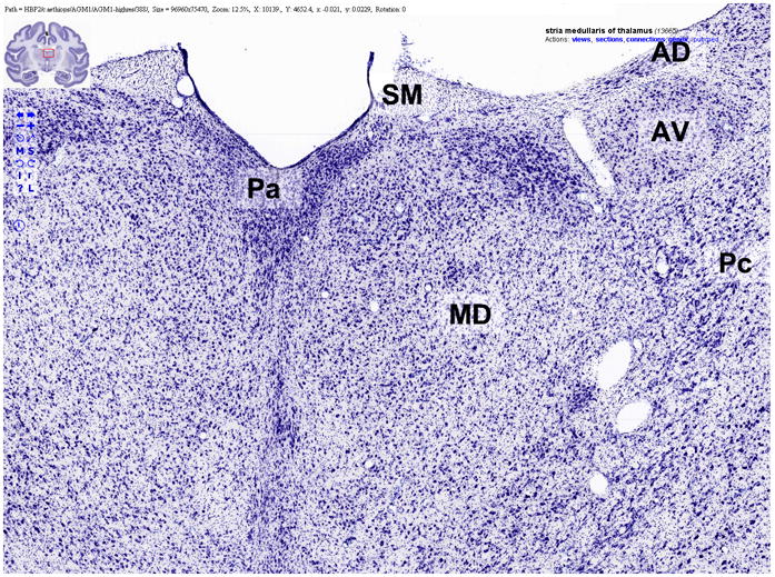
An example of a Flash-based graphical user interface for viewing high-resolution neuroanatomical images at BrainMaps.org. Note the overlaying labels (“Pa”, “MD”, “AD”, “AV”, “Pc”, and “SM”) and the label-specific context menu in the upper right that enables the user to retrieve related information, including the position of the label in the labeling hierarchy, connectivity, and patterns of gene expression.
2.7 Image Labeling
The terminology employed for online labeling of virtual slides is derived from that of Berman (1968), Berman and Jones (1982), Olszewski (1952), and Jones (1985, 2006). It incorporates many of the terms found in NeuroNames (Bowden & Martin, 1995) and other brain atlases, including the atlases of Swanson (1998), Paxinos, Toga, and Feng (2000), and Emmers and Akert (1963). A total of 19,702 labels were made. An example of labels overlaying a Nissl section is shown in Figure 6 for “Pa”, “MD”, “AD”, “AV”, “Pc” and “SM”, indicating the paraventricular, mediodorsal, anterodorsal, anteroventral, and paracentral nuclei of the thalamus, and the stria medullaris.
2.8 Speed of Online Image Accessibility
Figure 7 shows a 2D scatter plot with marginal histograms indicating tile fetch times (in ms) on the Y-axis and tile sizes (in kb) on the X-axis. The number of data points is 1000 and corresponds to a random selection of tiles in an image pyramid for a single monkey section of size 95,040 × 74,061 pixels. The mean image tile fetch time is 84.4 ms and the mean image tile size is 4.11 kb. From the tile size marginal histogram, there are two prominent peaks, with the one centered at 1–2 kb corresponding to non-tissue containing image tiles (which tend to be predominantly white and contain low frequency components), and the one centered at 12 kb corresponding to tissue-containing image tiles (which tend to contain high frequency components, such as cells). Note that tile fetch times are not related to tile size.
Figure 7.
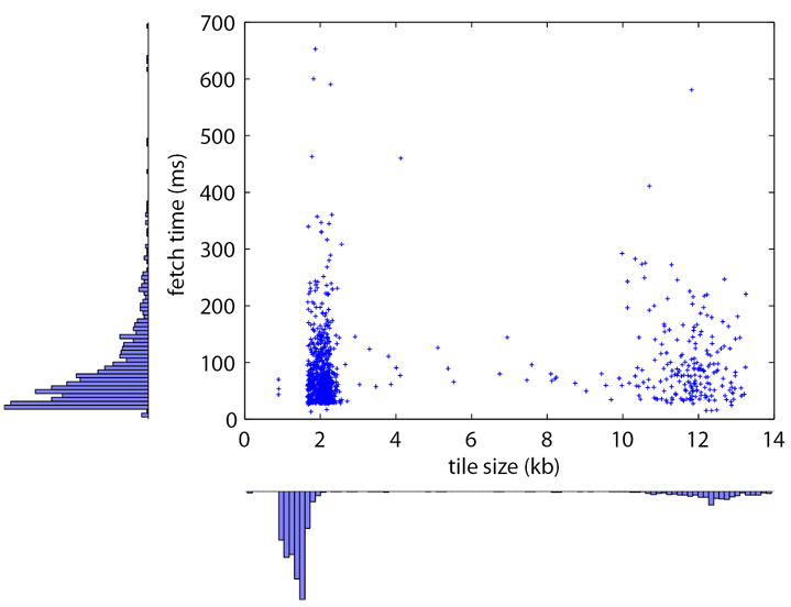
2D scatter plot with marginal histograms showing tile fetch times (in ms) on the Y-axis and tile sizes (in kb) on the X-axis. The number of data points is 1000 and corresponds to a random selection of tiles in an image pyramid for a single monkey section of size 95,040 × 74,061 pixels. The mean image tile fetch time is 84.4 ms and the mean image tile size is 4.11 kb.
3 Discussion
Prior to recent advances in virtual microscopy, slides were commonly digitized by various forms of film or flatbed scanner and image resolutions rarely exceeded 5000 dpi. Nowadays, it is possible to achieve more than 100,000 dpi and thus resolutions approaching that directly visible under the optical microscope. This increase in scanning resolution comes at a price: a typical flatbed or film scanner ranges in cost from $200 to $600; a 100,000 dpi slide scanner ranges from $80,000 to $100,000.
The virtual microscopy technology described in this manuscript first appeared two years ago and is currently offered by several companies, including Aperio (Aperio Technologies, Vista, CA, USA), MicrBrightField (MicroBrightField Inc, Williston, VT, USA), Zeiss (Carl Zeiss Inc), and Bacus Laboratories (Lombard, IL, USA). The virtual microscopy solutions offered by these companies vary. Aperio’s line scanning technology enables the fastest acquisition of virtual slides. In this paper, we have demonstrated that the technology scales to at least 10 million megapixels.
Scalability is an important issue. Scalability involves 1) image storage, 2) database storage, 3) visitor demands (or bandwidth), and 4) CPU. The most obvious question, when dealing with multi-terabyte image storage, is how will the server architecture (Figure 4) scale with increasing image storage requirements. With each LaCie external HDD disk array holding 2 terabytes, it is realistic to have over 35 terabytes on a single server (the upper limit is over 2 petabytes but space limitations make this unfeasible). To scale beyond 35 terabytes on a single server, it will be necessary to have multiple servers with multiple multi-terabyte image repositories, possibly geographically distributed. This is readily feasible with current technology, and would allow for almost unlimited scaling of image storage. The distributed nature of image storage would be invisible to an end-user, who would only see petabytes or more of image data accessible from an apparently centralized web location. Scaling with respect to database storage does not present a problem as most of the database storage would be for storing pointers to image locations (which may or may not be distributed and could reside on different servers). Consequently, the size of the database for storage of image locations would be very small and would not be expected to exceed one gigabyte, even for hundreds of thousands of virtual slides. Scaling with respect to visitor demands (or bandwidth) is not currently an issue with 1000 – 2000 unique users visiting BrainMaps.org on a daily basis to access virtual slides. However, it will be necessary to assess how well the server architecture (Figure 4) will scale with increasing visitor demands. Finally, there is the issue of scalability with respect to computer CPU. Our experience is that CPU demands are minimal and rarely exceed 1% even during peak visitor usage. Thus, we expect that scalability with respect to CPU will not be an issue in the foreseeable future. In sum, we expect our server architecture (Figure 4) to scale at least up to 35 terabytes of compressed image storage, and thereafter, that a distributed server and image storage solution can be readily implemented to accommodate potential petabyte-sized image storage and beyond.
How does the BrainMaps.org database, containing more than 10 million megapixels (or 35 terabytes), compare with other image databases? The Allen Brain Atlas (brain-map.org), featuring in situ hybridizations for 20,000 genes, contains 200,000 serial sections of the mouse brain at 100 megapixels per section, is estimated to have 20 million megapixels (or 60 terabytes). MicroBrightField’s neuroinformatica.com, which offers functionality in many respects similar to what is described here, is estimated to have less than 1 million megapixels. Perhaps the best known and arguably most massive image databases is Google Maps (maps.google.com), which provides high resolution satellite image data covering the entire earth, and is estimated to have 50–100 million megapixels (with an upper bound of 460 million megapixels). If the trend towards increasingly massive online image databases continues, we expect not only increasing numbers of online image databases of the kind that we describe here to appear, but also that the size of these databases will also increase. The largest image databases in existence today, including brainmaps.org, brain-map.org, and maps.google.com, are terabyte-size databases. Given the pace of technology, we can expect the appearance of petabyte-size image databases within the next 5–10 years. Neuroanatomical image databases of this size would contain more data than any individual lab could accumulate, and would necessitate the formation of a community of data contributors and sharers. The end-users would be the entire public. The implications of this massive sharing of neuroanatomical data have yet to be fully appreciated, particularly when additional tools are provided for visualization and neuroanatomical exploration of the data.
Virtual microscopy, although having many advantages, is unlikely to replace real microscopy any time soon. For one thing, it still depends on the preparation of conventional slides where quality must be controlled in the first instance by microscopic observation. For the time being, it nicely complements and extends the capabilities of real microscopes. Virtual microscopy, however, facilitates: 1) data-sharing and remote access, 2) data-management and annotation, and 3) various forms of data-mining. Data management and data-mining by microscopic observation of conventional slides are time-consuming and costly. Virtual (digitized) slides make this possible at minimal cost. The online distribution and sharing of virtual slides with anyone with an internet connection ensures the rapid dissemination and comparison of neuroanatomical data that is otherwise extremely difficult.
While virtual slides have many benefits, they also lack certain attributes. It is not possible to change focus in a virtual slide as it is in a real slide. For visualization, this is not a problem since the preparation of virtual slides tends to bring them into a single plane of focus. However, the inability to change the plane of focus in a virtual slide rules out its use in unbiased stereological estimation methods that require optical disectors (West & Gundersen, 1990). Nonetheless, biased stereological estimation methods, or unbiased methods not using optical disectors, are still possible. Another potential drawback is that the resolution of the virtual slide is limited to the optical lens used in the scanner. For example, if we generate a virtual slide at 20x and subsequently want to examine part of the slide at 40x, then it is necessary to rescan the entire slide using a higher power objective, which in some cases, is not possible due to file size restrictions or hardware issues. Finally, at the time of writing, virtual microscopy does not deal well with fluorescence because of low illumination and the bleaching of fluorophores during scanning.
Virtual microscopy-based digital brain atlases are superior to conventional print atlases in: 1) resolution, 2) annotation, 3) interaction, 4) data integration, and 5) the variety of data that can be obtained from them. The resolution of conventional print brain atlases typically does not exceed 7200 dpi, whereas virtual microscopy-based digital brain atlases attain 100,000 dpi and offer the ability to zoom in and out. Annotation can be more complete in virtual microscopy-based digital brain atlases, with options to display some types of annotations and make the rest invisible and it can be modified readily when necessary. Greater interactivity means that the user can zoom in/out and pan through brain image data, which is not possible in print-based atlases. Data-integration capabilities, including the integration of connectivity and gene expression data, are superior for the virtual microscopy-based digital brain atlases. And finally, the ability to extract other forms of data from virtual microscopy-based digital brain atlases, and from images of connection tracing and in situ hybridization section, is not available for print-based atlases. This kind of data-mining involves, for example, extraction of implicit, previously unknown, and potentially useful information and patterns from image data. An example could be the application of granulometry analysis for determining distributions of cell body sizes (assumed to be roughly spherical) throughout the brain. High-throughput image analysis is also possible through the use of programs that interact directly with the BrainMaps.org server. Many examples of such programs exist and certain ones are freely available at BrainMaps.org.
In summary, we have implemented a method for digitizing at microscopic resolution histological, histochemical, and immunocytochemical section data and making the content easily and conveniently accessible online. We have shown that web-accessible virtual microscopes and brain atlases can be developed using existing computer and internet technologies that offer universal data-sharing, and that rapid and seamless navigation through vast image datasets can be achieved using hierarchically-organized, multiresolution images in conjunction with a graphical user interface. By offering the possibility of interactively visualizing completely digitized brains at the sub-neuronal level, our online tools will prove useful for very large-scale histochemical, gene expression, and eventually stereological analyses. Our method will be straightforward to replicate by other labs seeking to increase accessibility and facilitate sharing of their neuroanatomical data.
Acknowledgments
We gratefully acknowledge Mr. Phong Nguyen for immunocytochemical and histochemical assistance, Matthew Countryman and Long Votran for annotation assistance, and Dr. Alessandro Graziano for manuscript review. Supported by Human Brain Project Grant Number MH60975 from the National Institutes of Health, United States Public Health Service.
5 Appendix
5.1 Image Tile Retrieval Example
Here we consider a detailed example from Section 2.3 of image tile retrieval. Consider the image pyramid of one of the monkey images, RH4-0801: From ImageProperties.xml, we make the following assignments: W=93707, H=70262, N=134841, and T=256. There are 10 Tiers, numbered 0 to 9 (⌈log2(max(93707, 70262)/256)⌉ + 1 = 9). The directory containing ImageProperties.xml itself contains directories TileGroup0 to TileGroup526. TileGroup0 contains files 0-0-0.jpg, 1-0-0.jpg to 1-1-1.jpg, 2-0-0.jpg to 2-2-2.jpg, 3-0-0.jpg to 3-5-4.jpg, 4-0-0.jpg to 4-11-8.jpg, and 5-0-0.jpg to 5-22-3.jpg. The remainder of the Tier 5 files are contained in TileGroup1 (256 files) and TileGroup2, which contains the remainder of Tier 5. The remainder of TileGroup2 contains 6-0-0.jpg up to 6-45-3.jpg for a total of 256 files. All of the TileGroup directories contain exactly 256 files with the possible exception of the last (TileGroup526 in this case), which will contain N mod 256 files, if this value is greater than zero; otherwise, it will contain the full 256 files. In this example, it contains 134841 mod 256 = 185 files.
Footnotes
Publisher's Disclaimer: This is a PDF file of an unedited manuscript that has been accepted for publication. As a service to our customers we are providing this early version of the manuscript. The manuscript will undergo copyediting, typesetting, and review of the resulting proof before it is published in its final citable form. Please note that during the production process errors may be discovered which could affect the content, and all legal disclaimers that apply to the journal pertain.
References
- Afework A. Digital Dynamic Telepathology: The Virtual Microscope. University of Maryland; 1998. [PMC free article] [PubMed] [Google Scholar]
- Berman AL. The Brain Stem of the Cat. University of Wisconsin Press; 1968. [Google Scholar]
- Berman AL, Jones EG. The thalamus and basal telencephalon of the cat: a cytoarchitectonic atlas with stereotaxic coordinates. University of Wisconsin Press; 1982. [Google Scholar]
- Bowden D, Martin R. NeuroNames Brain Hierarchy. Neuroimage. 1995;2(1):63–83. doi: 10.1006/nimg.1995.1009. [DOI] [PubMed] [Google Scholar]
- Emmers R, Akert K. A Stereotaxic Atlas of the Brain of the Squirrel Monkey (Saimiri Sciureus. Madison: Univ. of Wisconsin Press; 1963. [Google Scholar]
- Felten C, Strauss J, Okada D, Marchevsky A. Virtual microscopy: high resolution digital photomicrography as a tool for light microscopy simulation. Hum Pathol. 1999;30(4):477–83. doi: 10.1016/s0046-8177(99)90126-0. [DOI] [PubMed] [Google Scholar]
- Ferreira R, Moon B, Humphries J, Sussman A, Saltz J, Miller R, Demarzo A. The Virtual Microscope. Proceedings of the 1997 AMIA Annual Fall Symposium. 1997:449–453. [PMC free article] [PubMed] [Google Scholar]
- Jones EG. The Thalamus. Plenum Press; 1985. [Google Scholar]
- Jones EG. The Thalamus - Revisited. Cambridge University Press; 2006. [Google Scholar]
- Martone M, Gupta A, Ellisman M. e-Neuroscience: challenges and triumphs in integrating distributed data from molecules to brains. Nature Neuroscience. 2004;7(5):467–472. doi: 10.1038/nn1229. [DOI] [PubMed] [Google Scholar]
- Olszewski J. The Thalamus of the Macaca Mulatta; an Atlas for Use with the Stereotaxic Instrument. Basel; Karger: 1952. [Google Scholar]
- Paxinos G, Toga A, Feng X. The rhesus monkey brain in stereotaxic coordinates. Academic Press; 2000. [Google Scholar]
- Romer D, Suster S. Use of virtual microscopy for didactic live-audience presentation in anatomic pathology. Ann Diagn Pathol. 2003;7(1):67–72. doi: 10.1053/adpa.2003.50021. [DOI] [PubMed] [Google Scholar]
- Swanson LW. Brain Maps: Structure of the Rat Brain: a Laboratory Guide with Printed and Electronic Templates for Data, Models, and Schematics. Elsevier; 1998. [Google Scholar]
- West MJ, Gundersen HJG. Unbiased stereological estimation of the number of neurons in the human hippocampus. 1990 doi: 10.1002/cne.902960102. [DOI] [PubMed] [Google Scholar]