

Abstract
In continuous wave (CW) electron paramagnetic resonance imaging (EPRI), high quality of reconstructed image along with fast and reliable data acquisition is highly desirable for many biological applications. An accurate representation of uniform distribution of projection data is necessary to ensure high reconstruction quality. The current techniques for data acquisition suffer from nonuniformities or local anisotropies in the distribution of projection data and present a poor approximation of a true uniform and isotropic distribution. In this work, we have implemented a technique based on Quasi-Monte Carlo method to acquire projections with more uniform and isotropic distribution of data over a 3D acquisition space. The proposed technique exhibits improvements in the reconstruction quality in terms of both mean-square-error and visual judgment. The effectiveness of the suggested technique is demonstrated using computer simulations and 3D EPRI experiments. The technique is robust and exhibits consistent performance for different object configurations and orientations.
Keywords: Projection Acquisition, Artifacts, Reconstruction, EPRI
INTRODUCTION
Electron paramagnetic resonance imaging (EPRI) is a noninvasive technique that is capable of mapping the distribution of unpaired electrons [1,2]. It has a distinct advantage in many medical applications [3–5] where it can be used for the direct measurement of both endogenous and introduced free radicals which carry unpaired electrons. In the past few years, the potential applications of EPRI to studies of living biological systems have been recognized [6–9]. Despite all the progress made in the last two decades, the acquisition of high quality images of biological samples has been limited by several technical factors including resolution, sensitivity, and speed of data acquisition [10,11].
Most of the EPR experiments are conducted in continuous wave (CW) domain as the technical challenges associated with pulsed EPR [12] limit its broad use. In CW EPRI, the data are acquired in the form of projections [13], and filtered backprojection (FBP) [14] or Fourier based reconstruction techniques [15] are commonly used to reconstruct the image from the acquired projections. Quality of the reconstructed image depends on a number of factors such as number of acquired projections, sensitivity of the system, signal to noise ratio, field homogeneity, and linewidth of the paramagnetic species under study. In general, the reconstruction quality can be improved by acquiring a large number of projections. This, however, is not an attractive solution because projection acquisition can be a time consuming process [16], e.g., it may take several seconds to acquire a projection. Hence, increasing the number of acquired projections beyond a certain limit may not be practical especially for biological applications. Consequently, it is highly desirable to improve the reconstruction quality without acquiring further projections.
One important parameter to ensure an improved quality of the reconstructed image is the distribution of acquired projection data. Adaptive acquisition techniques have been proposed [17,18] to acquire a set of nonuniformly distributed projections which capture more vital and distinct information and hence result in reduced acquisition time. Although, the adaptive techniques tend to converge faster (generate lower mean-square-error (MSE) for same number of projections) than the uniform acquisition techniques, they are not suited to preserve weak signal [19]. Furthermore, the performance of the adaptive techniques is content-dependant and suited mostly for objects with highly anisotropic configurations. The performance of the uniform acquisition techniques, on the other hand, tends to be more robust and content-independent. The calculation of a uniform distribution of projections for 2D imaging is a trivial problem, but for 3D cases, the estimation of a uniform distribution of projections (gradient directions) is more complicated. The previously proposed uniform acquisition technique [17,20] offers an improvement over the conventional method of acquiring projections on a latitude-longitude grid by saving approximately 30% of the acquisition time, but it is still not an accurate approximation of a true uniform distribution of the gradient directions. In this work, we have shown that the reconstruction quality can be improved by adopting a more accurate representation of the uniform distribution of the projection data. The technique (for uniform distribution) described in this paper is based on a Quasi-Monte Carlo (QMC) method [21]. Such techniques have been frequently applied to simulate the behavior of various stochastic processes. Although the technique is explained for 3D spatial imaging, it can be readily extended to 3D spectral-spatial imaging. Extension of the suggested technique for 4D spectral spatial imaging is not straight forward and will be reported separately.
THEORY
In CW EPRI, the data are collected in the form of projections. A projection is acquired by measuring the absorption signal as a function of magnetic field in the presence of a static gradient. The orientation of the acquired projection is determined by the direction of the magnetic field gradient which is a vector sum of three independent and mutually orthogonal field gradients in the x, y, and z directions. The 3D radon transform [13] of an object f (x, y, z) is expressed as:
| (1) |
where p(r,θ,φ) represents an acquired projection along orientation defined by spherical coordinates θ, φ, and r. The distribution of θ and φ determines the distribution of projection data over the surface of a 3D sphere.
Once a sufficient number of projections are acquired, the image can be reconstructed by the FBP method. The FBP method requires that the gradient directions for the acquired projections are uniformly distributed over the 3D spatial domain. If the projections are not uniformly distributed, an appropriate weighting factor is used to validate the use of the FBP which is based on inverse Radon transform.
| (2) |
where pf represents a filtered projection and D represents the surface of a unit sphere. For a limited number of projections Eq. (2) can be approximated numerically by selecting a suitable distribution of sampling points.
| (3) |
The error of approximation (f− f̃) depends on the number of projections (n) and the distribution of the projections. Generally, a projection distribution which is more uniform over the sphere surface results in smaller approximation errors because there is a connection between better uniformity of data distribution and more accurate integration [22].
Equal linear angle sampling
For the traditional acquisition technique where θ and φ are arranged on a latitude-longitude grid as shown in Fig. 1A, reconstruction from the projections is described by Eq. (4), which is translated to Eq. (5) for a limited number of projections.
Figure 1.
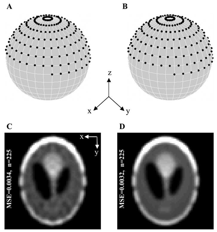
Effect of dislocating the gradient directions from a latitude-longitude grid on the reconstruction quality. A 3D Shepp-Logan phantom constructed by stacking (along z-axis) 2D Shepp-Logan phantom of size 64x64. (A) Distribution of 225 projections over a hemisphere using equal linear angle acquisition with Δθ= Δφ=π 15. All the projections corresponding to φ= 0 are identical regardless of the θ value. In order to avoid the acquisition of these identical projections, the angleφ is started from Δφ2 instead of 0. It should also be noted that the projections corresponding to φ=π 2 are only acquired for θϵ[ 0,π)since the symmetry of the projection data ensures that the other half(θϵ[ π, 2π)) is covered automatically. (B) Distribution of 225 projections after equal linear angle distribution given in A is modified by choosing a different set of azimuth angles for each iteration of mΔφ so that projection distribution does not follow the rigid latitude-longitude grid. (C) Center slice of image reconstructed using distribution given in A. (D) Center slice of image reconstructed using distribution given in B. From C to D, there is a visible reduction in the reconstruction artifacts suggesting that the isotropy of the data distribution results in an improved reconstruction quality.
| (4) |

An equal increment of θ and φ results in a nonuniform distribution of the data over the surface of the 3D sphere. The acquired data are highly concentrated near the poles and get sparse as we move towards the equator. The weighting term sin(mΔφ) K in Eq. (5) compensates for the nonuniform data distribution. As a result, the impact of a projection, which is near the pole (φ≈ 0), on the reconstruction is reduced. Since a projection near the pole requires the same amount of acquisition time as a projection near the equator, reducing the weighting of the projections near the pole results in the loss of data acquisition efficiency. In addition, sampling of data on a rigid latitude-longitude grid can lead to more pronounced reconstruction artifacts, because in such cases artifacts from various projections may get added constructively, which may have a degrading effect on the reconstruction quality. An improvement in the reconstruction quality can be achieved by dislocating the data points from the latitude-longitude grid which can be achieved by starting each iteration of φ from a different azimuth angle as shown in Fig. 1B. Even though the data points are still concentrated near the poles, a more isotropic coverage of 3D space is achieved by picking nonoverlapping sets of θ for each iteration of φ. Visual inspection of the simulation results presented in Fig. 1C and 1D illustrate that introducing a jitter in the angular distribution of the data can lower the reconstruction artifacts.
Equal solid angle sampling
A distribution based on equal solid angle approximation is shown in Fig. 2A. Since solid angle associated with gradient direction is proportional to ΔφxΔθx sin (φ), equal solid angle span [20] can be approximated by keeping Δφ constant and incrementing Δθ for each latitude ring in proportion to 1/sin(φ). This way, the number of azimuth samples for each φ is determined as:
Figure 2.

Distribution of gradient directions (A) 229 projection directions distributed using equal solid angle scheme. (B) 225 projection directions distributed using the suggested QMC-based acquisition technique.
| (6) |
where K is a constant that determines the total number of projections.
Therefore, as φ decreases (near the poles), the number of points also decreases accordingly which results in a more uniform distribution of the gradient directions. Consequently, for equal solid angle sampling Eq. (5) can be modified as:

As sin(mΔφ) Km ≈ 1 K, therefore from Eq. (7) it is evident that all the projections are weighted almost equally which results in an efficient data acquisition. Although the overall distribution of the gradient directions is more uniform as compared to the acquisition over a latitude-longitude grid, it still suffers from local anisotropies. Since the data distribution follows a pattern, it may exaggerate the reconstruction artifacts depending on the object configuration.
QMC-based sampling
QMC-based methods are often used in the numerical analysis for the computation of multidimensional integrals by using low discrepancy sequences [23]. This is in contrast to a regular Monte Carlo (MC) method which is based on the sequences of random or pseudorandom numbers. It has been shown that QMC-based distributions provide a better uniformity of data points than MC-based techniques [24]. Data uniformity is usually measured in terms of star discrepancy [25]. If is an infinite sequence of points in the interval [0, 1) and VN denotes the finite subsequence , star discrepancy, for each N, is defined as:
| (8) |
where N is the number of data points and sup |·| represents supremum [26].
The sequence V is uniformly distributed in [0, 1) if and only if . In this work, we are interested in sequences for which is small for all N. It has been shown [27] that for low discrepancy sequences the star discrepancy is bounded:
| (9) |
where d is the dimension in which the points of V lie and C is a constant that depends on d.
In QMC-based methods, since the samples are generated from a deterministic formula, they exhibit certain regularity properties of the distribution which is described by their discrepancy. As a result, these methods have leverage over MC methods in the sense that the bounds over the error magnitude are deterministic [21]. There are several algorithms available to generate low-discrepancy sequences [21]. In this work, we present a technique that is based on two successive Fibonacci numbers. Similar techniques have been presented before [28–30] for other applications. For the numerical integration on a sphere surface, there is a distinct advantage of using an oblique array of sampling points based on a chosen pair of successive Fibonacci numbers [31]. The pattern has a familiar appearance of intersecting spirals, avoiding the local anisotropy of a conventional latitude-longitude array which may result in enhanced reconstruction artifacts due to the coherent interaction between the data points.
For a high quality 3D reconstruction of the projection data, we are interested in a distribution of points on the surface of the hemisphere that is more uniform. The joint probability density function (p.d.f.) [32] of random variables Θ and Φ is given as:
| (10) |
The corresponding stochastic representation follows
| (11) |
| (12) |
where U1 and U2 represent uniform random variables in [0,1). It is the mechanism of selecting θ and φ that distinguishes QMC from MC method. For MC simulation of the data distribution, the points are selected randomly for U1 and U2. For QMC, the selection of θ and φ is deterministic and is based on two successive Fibonacci numbers. Pseudocode for generating uniformly distributed points, from two successive Fibonacci numbers, over the hemisphere surface is given by Eqs. (13–17). Figure 2B shows the distribution of 225 points generated using the QMC-based algorithm over a hemisphere. Once the projection are acquired along these orientations (θ and φ), the inverse Radon transform is applied to reconstruct a 3D image in a single stage, in which all the acquired projections are filtered and then back-projected directly on to the 3D image space.
| (13) |
where fk represents kth term of the Fibonacci sequence.
| (14) |
| (15) |
| (16) |
| (17) |
For an accurate distribution of the projection data, it is desirable for N and M to be successive Fibonacci numbers because of the strong irrationality of the inverse golden ratio , but it may restrict us from acquiring an arbitrary number of projections. This limitation can be relaxed by choosing N and M which are not necessarily Fibonacci numbers as long their ratio N/M stays close to the golden ratio. This approximation, however, may introduce discrepancy in the distribution of the projection data. Furthermore, the proposed algorithm does not take into account that 3D EPRI data is acquired over a hemisphere as opposed to a sphere since the symmetry ensures that the data on other hemisphere is acquired automatically. As a result, the QMC-based acquisition may introduce nonuniformity in the distribution of data along the junction of hemispheres. Fortunately, such discrepancies are limited in extent and do not have profound effects on the reconstruction quality, and therefore can be ignored if there are sufficient projections. Such nonuniformity in the distribution of the data, nevertheless, can be suppressed by applying a density compensation scheme, such as Voronoi diagram [33], where each projection is assigned a weight depending on its spherical distance from the neighboring projections.
The Voronoi diagrams are frequently used to segment a Euclidean space by determining the distances to a discrete set of points. Recently, the Voronoi diagrams have been used in MRI for density compensation [34] of the non-Cartesian k-space sampling such as spiral or radial. The non-Cartesian k-space sampling has an undesired property of nonuniform distribution of data over the k-space. The Voronoi diagram segments the k-space into convex polygons such that each polygon encloses only one data point, and all the points in the polygon are closer to the data point enclosed by the polygon than any other data point. The size of the each polygon can be used as the weight for the data point enclosed by the polygon. The same approach is applied here to calculate the weighting of the individual projections by calculating the Voronoi diagram over the surface of a sphere [35]. To accomplish that, the entire surface of the sphere is covered uniformly with the points selected using equal solid angle distribution. For accurate results, the number of points should be at least two orders of magnitude larger than the number of data points (projections). Now each of these uniformly distributed points is assigned to its closest (in terms of spherical distance) projection. Consequently, the relative weight of each projection equals the number of points assigned to it. These calculated weights for the projections are then normalized so that the average weight is one.
RESULTS
Simulations
To demonstrate the performance of the QMC-based isotropic distribution, the reconstruction results from the three acquisition techniques are compared using a digital phantom of size 64x64x64. The phantom consisted of six torus shaped configurations. The red color tori represent a normalized intensity of 1, while the yellow and the blue tori represent normalized intensities of 0.7 and 0.4 respectively. The reconstruction was performed for three orthogonal orientations of the phantom as shown in Fig. 3A. These orientations were achieved digitally by a 90° change in elevation angle (Fig. 3A, second column) followed by a 90° change in azimuth angle (Fig. 3A, third column). The imaging parameters were chosen to simulate EPRI experiments at L-band (1.2 GHz). All the simulations were performed using our EPRI simulation program written in Matlab (Mathworks, Massachusetts, USA). The imaging parameters in the simulation were as follows: field of view, 1.2x1.2x1.2 cm3; sweep width, 12 G; data points per projection, 120; gradient strength, 10 G/cm; width of Lorentzian lineshape, 300 mG. To simulate the experimental setup, deconvolution was performed on each projection using a Hanning window whose width was chosen empirically.
Figure 3.

Reconstruction results of a simulated phantom using the three acquisition techniques for three orthogonal orientations of a phantom (see text for the description of the phantom). (A) Three orthogonal orientations of the simulated phantom which consists of six torus-shaped objects. (B) Reconstruction of A based on equal linear angle acquisition with 225 projections. (C) Reconstruction of A based on equal solid angle acquisition with 229 projections. (D) Reconstruction of A using the QMC-based acquisition with 225 projections. For proper display, voxels with intensity less than the 25% of the peak intensity of the reconstructed image were set to zero. In addition, all the reconstructed images were cropped from the center for better visualization.
Figures 3B, 3C, and 3D show the reconstructed images for the three given phantom orientations using equal linear angle acquisition, equal solid angle acquisition, and the QMC-based angle selection, respectively, with 225 projections. The voxels with signal intensity less than 25% of the maximum intensity of the reconstructed image were set to zero. The results presented in Fig. 3 suggest that the isotropic distribution of the data for the QMC-based technique translates to a performance which is more consistent, predictable, and content independent. On the other hand, the performances of equal linear angle increment and equal solid angle increment techniques are more content dependant, e.g., the reconstruction based on equal solid angle acquisition generates reasonable results for the first orientation of the phantom (first column of Fig. 3C) while the reconstruction of same phantom, for identical imaging parameters, suffers from enhanced reconstruction artifacts for the second orientation (second column of Fig. 3C). Moreover, Fig. 4 shows that the QMC-based method generates lower MSE as compared to other two acquisition techniques for same number of acquired projections. For simplicity we have used MSE, along with the visual judgment, as a figure of merit. It should be noted that although MSE is commonly used to quantify the overall reconstruction quality, it may not express all aspects of the reconstruction quality such as spatial resolution or maximum error.
Figure 4.

MSE convergence for the three acquisition techniques. Number of projections vs. MSE for the phantom orientation shown in: (A) first column of Fig. 3A, (B) second column of Fig. 3A, and (C) third column of Fig. 3A. Here, ELA, ESA, and QMC stand for equal linear angle, equal solid angle, and the Quasi-Monte Carlo based acquisition, respectively.
EPRI experiment
For validation of the technique, an experimental phantom was constructed with 21 capillary tubes arranged in 3 rows and 7 columns as shown in Fig. 5. Each capillary tube had an inner diameter of 0.9 mm and an outer diameter of 1.4 mm. The tubes were filled to a height of 10 mm with Triarylmethyl radical TAM (0.7 mM) dissolved in PBS (phosphate buffer saline). Overall sample dimensions were 4.2 mm x 9.8 mm x 10 mm.
Figure 5.

Experimental phantom used for 3D EPRI experiment. A total of 21 capillary tubes were glued together so that they were arranged on a 7x3 grid. Each capillary tube had an inner diameter of 0.9 mm and an outer diameter of 1.4 mm. A 0.7 mM TAM solution was used to fill each capillary tube to a height of 10 mm. Sample dimensions were approximately 4.2 mm x 9.8 mm x 10 mm.
The phantom was imaged on an L-Band (1.2 GHz) EPRI system with a volume resonator with diameter of 12.57 mm and useable height of 12 mm. Spectrometer settings were: incident microwave power 4 mW, sweep width 12 G, modulation amplitude 0.15 G, scan time 5.24 s, and gradient strength 6 G/cm. The measured linewidth of the signal was 280 mG. Deconvolution, using Hanning low-pass window, was applied to individual projections to improve resolution. The cutoff frequency of the window was selected empirically. The measured SNR, defined as the ratio of peak signal amplitude to peak noise amplitude for the zero-gradient projection was 250. For each projection, 1024 data points per collected. No correction for B1 field inhomogeneities [36] was applied. A total of nine datasets were acquired using the parameter values listed above such that there were three datasets for each acquisition technique for three different numbers of projections. For equal linear angle acquisition, three datasets were acquired with 169, 256, and 576 projections, for equal solid angle acquisition, three datasets were acquired with 163, 254, and 499 projections, and for the QMC-based acquisition, three datasets were acquired with 165, 254, and 497 projections.
The reconstruction results from the three acquisition techniques, presented in Fig. 6, suggest an improvement in the reconstruction quality for the QMC-based acquisition technique. The reference image to calculate MSE was constructed from 1124 projections acquired using equal solid angle acquisition. The QMC-based acquisition technique generates lower MSE than other two acquisition techniques and gives consistent performance for different number of projections. On the other hand, the reconstructions based on the equal linear angle and equal solid angle techniques exhibit artifacts depending on the data distribution for a given object configuration. Depending on the configuration of the object, the more informative projections may be localized to a certain range of θ and φ. Both equal linear angle and equal solid angle based acquisitions have the tendency to skip that range of orientations altogether because of the large structured gaps in the data distribution. As a result, the performances of these techniques are hard to predict for arbitrary shaped objects. For instance, an increase in the number of acquired projections may result in further deterioration of the reconstruction quality if the corresponding projections do not capture the vital orientations that were initially covered by fewer projections. This may also explain the degradation in the image quality for equal linear angle and equal solid angle acquisition in Fig. 6A and 6B for the first two columns. On the other hand, the isotropic distribution of the projection data for QMC-based sampling is less susceptible to the mismatch of the sampling pattern and the orientations of the more informative projections.
Figure 6.
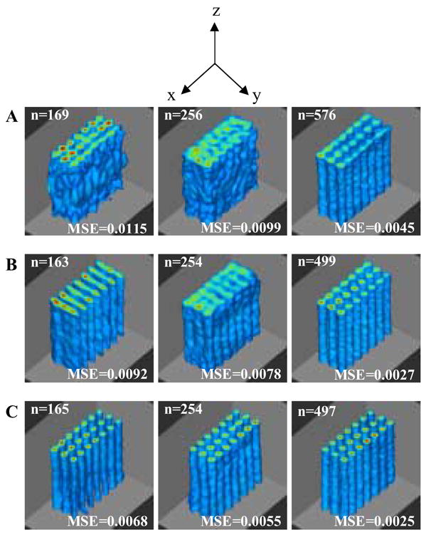
Reconstruction results for 3D EPRI of the capillary tubes phantom (shown in Fig. 5) to evaluate the performance of three different acquisition techniques. The measurements were performed on an L-band (1.2 GHz) EPRI system. Reconstruction results based on: (A) equal linear angle acquisition, (B) equal solid angle acquisition, and (C) the QMC-based acquisition for three different numbers of projections. Top 10% of the tubes were cropped for better visualization. Voxels with intensity less than the 25% of the peak intensity of the reconstructed image were set to zero.
DISCUSSION
The uniform isotropic coverage of 3D space is important for an optimized reconstruction quality. A poor approximation of the uniform distribution, on the other hand, may result in pronounced artifacts in the reconstructed image which may degrade the reconstruction quality to an unacceptable level. Although, equal solid angle acquisition provides an improvement over equal linear angle acquisition, it still suffers from local anisotropies in the distribution of gradient directions which may manifest themselves as enhanced artifacts in the reconstructed image. Both the simulations and the EPRI results indicate that the QMC-based uniform distribution of the gradient directions results in an improved image quality in terms of both MSE and visual inspection.
For the simulation data, the performance of the pre-existing data acquisition techniques, for identical imaging parameters, varies considerably for different orientations of the input phantom which implies that depending on the configuration, these techniques may require extra projections to generate similar reconstruction quality. On the other hand, the performance of the QMC-based technique is more consistent and independent of the phantom orientation. Visual inspection also reveals that the images reconstructed using the suggested acquisition technique exhibit lesser artifacts which in turn is effective in preserving the weak signal (blue tori). In addition, the suggested acquisition technique generates considerably lower MSE (Fig. 5) for all three orientations, and the difference is substantial especially at lower number projections. Likewise, the results from 3D EPRI experiment show that the reconstruction quality can be improved by acquiring the projections using the QMC-based acquisition. Figure 6 demonstrates that the reconstruction from the proposed acquisition technique exhibits lesser artifacts and generates lower MSE. For example, the MSE for the QMC-based technique with 165 projections is lower than the MSE generated by the other two acquisition techniques with more than 250 projections. The computation cost of the technique is low, e.g., in Matlab it takes couple of seconds to find an array of uniformly distributed gradient directions for 1000 projections.
CONCLUSIONS
A QMC based technique is suggested for a better approximation of the uniform distribution of projection data. The performance of the technique is compared to the existing techniques using both the computer simulations and the data from EPRI experiment. The results suggest an improvement, both qualitatively and quantitatively, in the reconstruction quality for the acquisition based on the suggested technique. Moreover, the performance of the QMC-based technique is more consistent and predictable. The technique is presented for 3D spatial imaging and can be extended to 3D spectral-spatial imaging.
Acknowledgments
This work was supported by NIH Grant EB005004 and NSF upon Agreement No. 0112050. We thank Sergey Petryakov for technical assistance.
Footnotes
Publisher's Disclaimer: This is a PDF file of an unedited manuscript that has been accepted for publication. As a service to our customers we are providing this early version of the manuscript. The manuscript will undergo copyediting, typesetting, and review of the resulting proof before it is published in its final citable form. Please note that during the production process errors may be discovered which could affect the content, and all legal disclaimers that apply to the journal pertain.
References
- 1.Fujii H, Berliner LJ. One- and two-dimensional EPR imaging studies on phantoms and plant specimens. Magn Reson Med. 1985;2:275–82. doi: 10.1002/mrm.1910020310. [DOI] [PubMed] [Google Scholar]
- 2.Ferrari M, Quaresima V, Sotgiu A. Present status of electron paramagnetic resonance (EPR) spectroscopy/imaging for free radical detection. Pflugers Arch. 1996;431:R267–8. doi: 10.1007/BF02346371. [DOI] [PubMed] [Google Scholar]
- 3.Fuchs J, Freisleben HJ, Groth N, Herrling T, Zimmer G, Milbradt R, Packer L. One- and two-dimensional electron paramagnetic resonance imaging in skin. Free Radic Res Commun. 1991;15:245–53. doi: 10.3109/10715769109105220. [DOI] [PubMed] [Google Scholar]
- 4.Hochi A, Furusawa M, Ikeya M. Applications of microwave scanning ESR microscope: human tooth with metal. Appl Radiat Isot. 1993;44:401–5. doi: 10.1016/0969-8043(93)90256-a. [DOI] [PubMed] [Google Scholar]
- 5.Kuppusamy P. EPR spectroscopy in biology and medicine. Antioxid Redox Signal. 2004;6:583–5. doi: 10.1089/152308604773934332. [DOI] [PubMed] [Google Scholar]
- 6.Kuppusamy P, Shankar RA, Roubaud VM, Zweier JL. Whole body detection and imaging of nitric oxide generation in mice following cardiopulmonary arrest: detection of intrinsic nitrosoheme complexes. Magn Reson Med. 2001;45:700–7. doi: 10.1002/mrm.1093. [DOI] [PubMed] [Google Scholar]
- 7.Matsumoto A, Matsumoto S, Sowers AL, Koscielniak JW, Trigg NJ, Kuppusamy P, Mitchell JB, Subramanian S, Krishna MC, Matsumoto K. Absolute oxygen tension (pO(2)) in murine fatty and muscle tissue as determined by EPR. Magn Reson Med. 2005;54:1530–5. doi: 10.1002/mrm.20714. [DOI] [PubMed] [Google Scholar]
- 8.Rolett EL, Azzawi A, Liu KJ, Yongbi MN, Swartz HM, Dunn JF. Critical oxygen tension in rat brain: a combined (31)P-NMR and EPR oximetry study. Am J Physiol Regul Integr Comp Physiol. 2000;279:R9–R16. doi: 10.1152/ajpregu.2000.279.1.R9. [DOI] [PubMed] [Google Scholar]
- 9.Velayutham M, Li H, Kuppusamy P, Zweier JL. Mapping ischemic risk region and necrosis in the isolated heart using EPR imaging. Magn Reson Med. 2003;49:1181–7. doi: 10.1002/mrm.10473. [DOI] [PubMed] [Google Scholar]
- 10.Deng Y, He G, Petryakov S, Kuppusamy P, Zweier JL. Fast EPR imaging at 300 MHz using spinning magnetic field gradients. J Magn Reson. 2004;168:220–7. doi: 10.1016/j.jmr.2004.02.012. [DOI] [PubMed] [Google Scholar]
- 11.Joshi JP, Ballard JR, Rinard GA, Quine RW, Eaton SS, Eaton GR. Rapid-scan EPR with triangular scans and fourier deconvolution to recover the slow-scan spectrum. J Magn Reson. 2005;175:44–51. doi: 10.1016/j.jmr.2005.03.013. [DOI] [PubMed] [Google Scholar]
- 12.Bourg J, Krishna MC, Mitchell JB, Tschudin RG, Pohida TJ, Friauf WS, Smith PD, Metcalfe J, Harrington F, Subramanian S. Radiofrequency FT EPR spectroscopy and imaging. J Magn Reson B. 1993;102:112–5. [Google Scholar]
- 13.Deans SR. The Radon transform and some of its applications. Wiley; New York: 1983. [Google Scholar]
- 14.Shepp LA, Logan BF. The Fourier reconstruction of a head section. IEEE Trans Nucl Sci. 1974;21:21–42. [Google Scholar]
- 15.Cho ZH, Jones JP, Singh M. Foundations of Medical Imaging. Wiley; New York: 1993. [Google Scholar]
- 16.Kuppusamy P, Chzhan M, Zweier JL. Development and optimization of three-dimensional spatial EPR imaging for biological organs and tissues. J Magn Reson B. 1995;106:122–30. doi: 10.1006/jmrb.1995.1022. [DOI] [PubMed] [Google Scholar]
- 17.Deng Y, Kuppusamy P, Zweier JL. Progressive EPR imaging with adaptive projection acquisition. J Magn Reson. 2005;174:177–87. doi: 10.1016/j.jmr.2005.01.019. [DOI] [PMC free article] [PubMed] [Google Scholar]
- 18.Placidi G, Alecci M, Sotgiu A. Theory of adaptive acquisition method for image reconstruction from projections and application to EPR imaging. J Magn Reson. 1995;108:55–7. [Google Scholar]
- 19.Ahmad R, Clymer B, Deng Y, He G, Vikram D, Kuppusamy P, Zweier JL. Optimization of data acquisition for EPR imaging. J Magn Reson. 2006;179:263–72. doi: 10.1016/j.jmr.2005.12.013. [DOI] [PubMed] [Google Scholar]
- 20.Lai CM, Lauterbur PC. A gradient control device for complete three-dimensional nuclear magnetic resonance zeugmatographic imaging. J Phys E: Sci Instrum. 1980;13 [Google Scholar]
- 21.Niederreiter H. Random number generation and quasi-Monte Carlo methods. Soc. Ind. Appl. Math; Philadelphia, Pa: 1992. [Google Scholar]
- 22.Hlawka E. Funktionen von beschränkter Variation in der Theorie der Gleichverteilung. Annali di Matematica Pura ed Applicata. 1961;54:325–33. [Google Scholar]
- 23.Shirley P. Proc Eurographics. Vol. 91. North-Holland: 1991. Discrepancy as a quality measure for sample distributions; pp. 183–93. [Google Scholar]
- 24.Papageorgiou A, Traub JG. Faster Evaluation of Multidimensional Integrals. Comput Phys. 1997;11:574–8. [Google Scholar]
- 25.Drmota M, Tichy RF. Sequences, discrepancies and applications, Lecture Notes in Math. Springer; Berlin: 1997. [Google Scholar]
- 26.Pyke R. The Supremum and Infimum of the Poisson Process. The Annals of Mathematical Statistics. 1959;30:568–76. [Google Scholar]
- 27.Thiémard E. An algorithm to compute bounds for the star discrepancy. J Complexity. 2001;17:850–80. [Google Scholar]
- 28.Mathé P, Wei G. Quasi-Monte Carlo integration over Rd. Math Comp. 2004;73:827–41. [Google Scholar]
- 29.Niederreiter H, Sloan IH. Integration of non-periodic functions of two variables by Fibonacci lattice rules. J Comp Appl Math. 1994;51:57–70. [Google Scholar]
- 30.Tezuka S, Fushimi M. Fast generation of low discrepancy points based on Fibonacci polynomials. Proc. 24th Winter Simul. Conf; Virginia. 1992. pp. 433–7. [Google Scholar]
- 31.Hannay JH, Nye JF. Fibonacci numerical integration on a sphere. J Phys A: Math Gen. 2004;37:11591–601. [Google Scholar]
- 32.Stark H, Woods JW. Probability and random processes with applications to signal processing. Prentice Hall; Upper Saddle River, N.J: 2002. [Google Scholar]
- 33.Aurenhammer F. Voronoi diagrams - a survey of a fundamental geometric data structure. ACM Comput Surveys. 1991;23:345–405. [Google Scholar]
- 34.Rasche V, Proksa R, Sinkus R, Bornert P, Eggers H. Resampling of data between arbitrary grids using convolution interpolation. IEEE Trans Med Imag. 1999;18:385–92. doi: 10.1109/42.774166. [DOI] [PubMed] [Google Scholar]
- 35.Na HS, Lee CN, Cheong O. Voronoi diagrams on the sphere. Comput Geom: Theory Appl. 2002;23:183–94. [Google Scholar]
- 36.He G, Evalappan SP, Hirata H, Deng Y, Petryakov S, Kuppusamy P, Zweier JL. Mapping of the B1 field distribution of a surface coil resonator using EPR imaging. Magn Reson Med. 2002;48:1057–62. doi: 10.1002/mrm.10302. [DOI] [PubMed] [Google Scholar]