

Abstract
The macaque striate cortex (V1) contains neurons that respond preferentially to various hues. The properties of these hue-selective neurons have been studied extensively at the single-unit level, but it is unclear how stimulus hue is represented by the distribution of activity across neuronal populations in V1. Here we use the intrinsic optical signal to image V1 responses to spatially uniform stimuli of various hues. We found that 1) Each of these stimuli activates an array of patches in the supragranular layers of the parafoveal V1; 2) The patches activated by different hues overlapped partially; 3) The peak locations of these patches were determined by stimulus hue. The peaks associated with various hues form well-separated clusters, in which nearby peaks represent perceptually similar hues. Each cluster represents a full gamut of hue in a small cortical area (∼160 μm long). The hue order is preserved within each peak cluster, but the clusters have various geometrical shapes. These clusters were co-localized with regions that responded preferentially to chromatic gratings compared with achromatic ones. Our results suggest that V1 contains an array of hue maps, in which the hue of a stimulus is represented by the location of the peak response to the stimulus. The orderly, organized hue maps in V1, together with the recently discovered hue maps in the extrastriate cortical area V2, are likely to play an important role in hue perception in primates.
Keywords: striate cortex, primate, color, map, perception, optical imaging
Introduction
The macaque striate cortex (V1) may play an important role in transforming the cone-specific inputs from the lateral geniculate nucleus into signals that are more specific for color perception (Hanazawa et al., 2000; Conway, 2001; Johnson et al., 2001; Wachtler et al., 2003). Numerous studies have focused on the receptive field properties and spatial organization of individual color-selective cells in V1, and have generated important hypotheses regarding cortical processing of color information (for reviews, see Shapley and Hawken, 2002; Lennie and Movshon, 2005). However, the responses of a neuron to repeated presentations of a given stimulus are variable (Schiller et al., 1976; Dean, 1981; Snowden et al., 1992; Croner et al., 1993; Gur and Snodderly, 1997; Kara et al., 2000; Gur and Snodderly, 2006). In addition, many neurons in V1 are selective for more than one attributes of a stimulus (Leventhal et al., 1995; Johnson et al., 2001; Friedman et al., 2003). In order to reliably extract information about a particular attribute of a stimulus from a single trial, a subject may rely on information coded in the spatiotemporal pattern of activity across neuronal populations. So far, it is unclear how information about color is coded in this pattern of activity in V1.
A Previous study has found that extrastriate cortical area V2 encodes information about stimulus color in the spatial distribution of activity across neuronal populations (Xiao et al., 2003). This finding raised the possibility that stimulus color might be coded by the spatial distribution of activity across V1 as well. To explore this possibility, imaging techniques and stimuli consisting of individual colors, rather than pairs of opponent colors, are required. One such study using the 14C-2-deoxy-d-glucose (2DG) technique found that stimuli of diffuse color activated an array of patches in both supragranular and infragranular layers (Tootell et al., 1988b). Regardless of the stimulus color, the peak region of these activated patches all overlapped with the cytochrome oxidase (CO) blobs, a compartment that has been hypothesized to play a particularly important role in color processing (Livingstone and Hubel, 1984; Ts'o and Gilbert, 1988). However, because the 2DG technique at that time could not be used to visualize the response of a cortical region to more than one stimulus, that study did not examine fine-scale spatial relationships among the activation patches associated with several colors.
An earlier study from our lab used intrinsic optical imaging, and found that color gratings also activated an array of patches in V1 (Orbach et al., 1996). The patches associated with different colors partially overlapped, but were centered at different locations. However, the spatial resolution of images in that study was relatively low (>50 μm/pixel). In addition, that study used colored gratings as stimuli. Since the orientation of gratings affects the spatial distribution of activity in V1 (Blasdel and Salama, 1986), it was difficult to interpret the results of that study regarding the coding of stimulus color by this spatial distribution.
In the current study, we used spatially uniform colored stimuli, and imaged the intrinsic optical signal at a very high spatial resolution. Our results suggest a possible mechanism by which the spatial distribution of V1 activity represents stimulus color.
Materials and Methods
Physiological Preparation
Experiments were carried out on four anesthetized monkeys (Macaca fascicularis). All procedures were approved by the local institutional Animal Welfare Committee, and were in full compliance with the NIH guidelines for the use of laboratory animals. Anesthesia was induced by ketamine (10 mg/kg), and continued with a mixture of propofol (4 mg/kg/h) and sufentanil citrate (0.05 μg/kg/h). Paralysis was maintained with pancuronium bromide (0.25 mg/kg/h) to prevent eye movements. End tidal CO2 was maintained at 32 mmHg (∼4.5%) and the body temperature was kept at 37.3°C, Blood pressure and EKG were continuously monitored to assure adequate anesthesia. A craniotomy and durotomy exposed the dorsal portion of V1 that represents retinal eccentricities of 1.5-5°. A recording chamber was installed over the exposed cortex, filled with silicon oil and sealed with glass during imaging.
Visual Stimulation
Visual stimuli were presented on a Sony GDM-400PS color monitor (refresh rate: 100 or 60 Hz, resolution: 640×480 or 1024×768), placed at a distance of 57 cm, which covered a 36° × 27° of the visual field, and centered on the fovea of the tested eye with a modified fundus camera. Phosphor emission spectra of the monitor were measured at 4 nm intervals using a spectraradiometer (PR-650, Photoresearch, CA). The monitor was driven by a VSG graphics card (Cambridge Research Systems, United Kingdom). Gamma correction was performed using the VSG software and the OptiCAL photometer (Cambridge Research Systems). Spatially uniform colors or gray was presented on the entire screen, and were all photometrically isoluminant (9.5 cd/m2). The CIE 1931-xy coordinates of the tested stimuli were: red(R) (0.55, 0.33), orange(O) (0.54, 0.40), yellow(Y) (0.45, 0.47), lime(L) (0.35, 0.54), green lime (GL) (0.28,0.61), green(G) (0.27, 0.49), aqua(A) (0.23, 0.36), blue(B) (0.16, 0.08), purple(P) (0.23, 0.12), reddish purple(RP) (0.31,0.17), pink(K) (0.38, 0.27) or (0.43, 0.24), and gray(W) (0.32, 0.32) or (0.35, 0.32). The letters in parentheses are abbreviations of the color names that are shown in Fig. 1A, which illustrates the location of all our stimuli on a CIE 1931-xy diagram. The CIE-xy coordinates of the three phosphors (red, green, blue) of the CRT were (0.62, 0.35), (0.28, 0.61), and (0.15, 0.07), respectively. The hue angel of each stimulus color, or huv as defined in the CIE 1976 (L*u*v*)-space, was calculated according to Wyszecki (1982). The CIE illuminant C was used as the white object-color stimulus in that calculation.
Fig. 1.
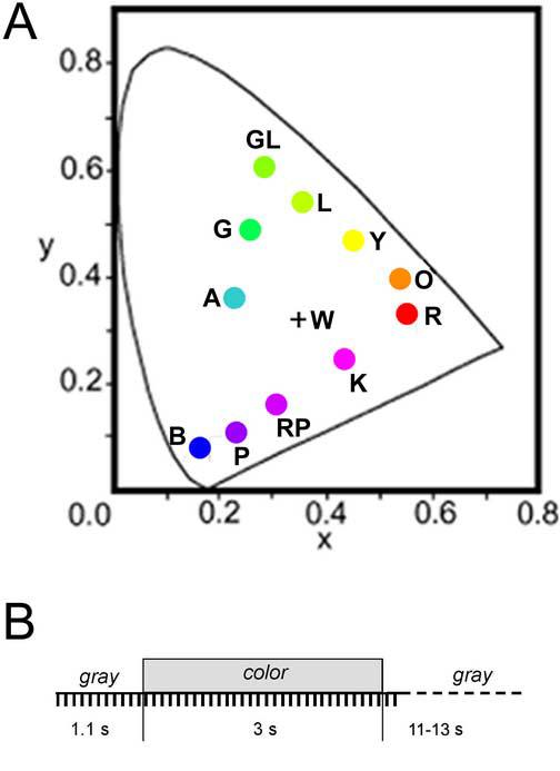
A: CIE 1931-xy coordinates of the stimulus colors. R, red; O, Orange; Y, Yellow; L, Lime; GL, green-lime; G, green; A, aqua; B, blue; P, purple; RP, reddish purple; K, pink; W, gray. B: A schematic depiction of the experimental protocol, showing the temporal sequence of stimulus presentation and data acquisition. Each tick mark indicates the time at which a cortical image was acquired.
To visualize the previously reported color patches that respond preferentially to chromatic grating compared with achromatic ones, responses to photometrically isoluminant red/green gratings were compared with those to black/white gratings (Roe and Ts'o, 1999; Landisman and Ts'o, 2002a). Both types of gratings had the same spatial and temporal frequencies (0.5 cycle/degree, 2 cycle/sec, square wave), and were presented at two alternating orientations (horizontal and vertical). The two colors in the red/green gratings are those of the red and green phosphors of the CRT, respectively.
The stimuli were presented either to the contra-lateral eye or to both eyes. In one animal that had a glaucomatous eye, the stimuli were presented to the normal eye.
Optical Imaging and data analysis
The intrinsic optical signal was recorded using a CCD camera with 652×492 pixels (PlutoCCD, PixelVision, OR, which has a 2×2 set of CCD detectors). The camera was focused 0–400μm below the cortical surface by a tandem lens macroscope (Ratzlaff and Grinvald, 1991). The camera took 10 frames/second at a resolution of 6.1 μm/pixel. The cortex was illuminated by 610 (+/− 8) nm light from LEDs driven by a stabilized power supply.
During each imaging trial, 11 frames were taken before, 30 during, and 2 after the 3-second presentation of a stimulus, followed by a rest period of 11-13 seconds, during which the display was uniformly gray (Fig. 1B). In two earlier experiments (Cases 1 and 2) that generated panels M-N and O-P of Fig. 6, respectively, 18 frames were taken during the 1.8-second presentation of a stimulus. An imaging block consisted of one imaging trial for each stimulus, including a control trial without stimulation, presented in a pseudo-random order. Functional maps were derived from an experiment consisting of 50-51 imaging blocks. To test the reproducibility of the functional images, the red stimulus was repeated twice in each imaging block.
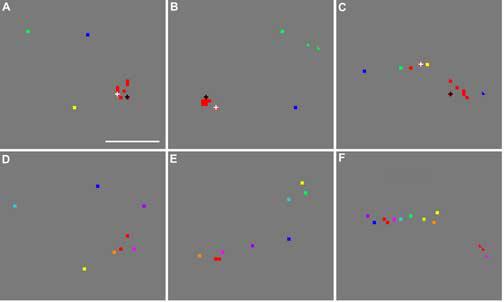
Fig. 6.
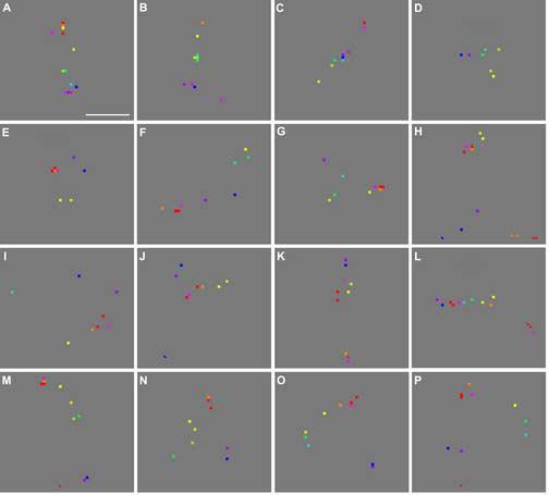
Clusters of response peaks imaged in additional experiments. (A)-(D) Clusters imaged in the same cortical area shown in Fig. 2, but here imaged during binocular stimulation. (E)-(L) Clusters imaged in Case 3, using monocular stimulation. (M)-(N) Clusters imaged in Case 2, using binocular stimulation. (O)-(P) Clusters imaged in Case 1, using monocular stimulation. Scale bar: 100 μm.
For each imaging trial, we calculated the average of 11 pre-stimulation frames and the average of the last 7 frames (5 during-stimulation frames and 2 after-stimulation ones). They are called pre-stimulation frames and response frames, respectively. To calculate a ‘single-condition’ image that represents the change in surface reflectance elicited by a given stimulus, we averaged the pre-stimulation frames and the response frames across all trials associated with the given stimulus. A ‘single-condition’ image was calculated by (Fr−Fp)/Fp, where Fr and Fp stand for the final average response frame and the final average pre-stimulation frame, respectively. A differential image was calculated by subtracting the single-condition image associated with one stimulus from that associated with another stimulus. Single-condition or differential images were then band-pass filtered by a Difference of Gaussian (DOG) filter (σ1=42.7 μm and σ2=331.8 μm) to remove both high frequency noise and very low frequency gradients. This filter also reduced the global intrinsic signal that is not specific to the stimulus (Frostig et al, 1990). It has been shown that the signal in a filtered single-condition image is highly correlated with the local neural activity (Meister and Bonhoeffer, 2001; Tsunoda et al., 2001; Xiao et al., 2003).
To estimate the statistical significance of each pixel's response to a given stimulus, we first filtered the pre-stimulation and response frames by the same DOG filter described above, and then calculated the paired t-value for each pixel based on all 50 or 51 pairs of pre-stimulation frames and response frames associated with that stimulus. A pixel is said to be significantly activated by a stimulus if the corresponding t-value is below −4.721 (for n=50) or −4.711 (for n=51), which corresponds to a significance level of P<10−5 (one tail). We used this P threshold that is more stringent than 0.05 as a correction for multiple comparisons. But it is less stringent than that calculated from the Bonferroni correction which may increase the risk of a type II error (not detecting activated pixels). By definition, the t-value of a pixel is also the signal-to-noise (S/N) ratio of the single-condition image at that pixel. By choosing a relatively high threshold of t-value, we have concentrated our study on regions with high S/N ratio.
Because intrinsic optical signals increase monotonically during the first three seconds of stimulation (Malonek and Grinvald, 1996; Xiao et al., 2003), the S/N ratio in the earlier experiments (Case 1 and 2) that used shorter stimuli (1.8 seconds) was lower compared with later experiments that used longer stimuli (3 seconds). As a consequence, these earlier experiments visualized fewer activated patches in response to each stimulus (especially the mid-spectral colors), compared with later experiments.
To locate the peak(s) in each response patch, the local minima were identified in a single-condition image. The local minima represent pixels with the most negative values, which correspond to the strongest neural response. Only the minima whose corresponding t-values passed the threshold described above were included in subsequent analyses of response peaks. The location of each response peak was marked with a square or a triangle of a color that is close to the color of the associated stimulus. These marking colors are illustrated in Fig. 1 as the color of circles that specify the CIE-xy coordinates. When two response peaks associated with different stimuli were located at the same pixel, one of these peaks was marked at the adjacent pixel for the purpose of illustration.
To exclude the response peak located on or near large blood vessels, the following procedures were performed. First, large blood vessels (> 30 μm) were identified on images of the cortical surface that were taken under green (570 nm) illumination. When the focal plane was not parallel to the cortical surface, successive images were taken, each focusing on different part of the surface. Second, any peak near (< 43 μm) or on the identified large blood vessels was excluded from further analysis. In this step, one of the raw images that generated the functional images was used to estimate the edges of each large blood vessel. The surface images were not used in this step because the functional images were derived from raw images that were taken at a deeper focal plane. This difference in focal plane caused a slight mismatch between the functional images and the surface ones. However, to illustrate the vasculature pattern more clearly, two surface images are shown in Fig. 5 and Fig. 11, overlaid with their corresponding peak maps. The selection of the images to be rejected was performed by a naive observer who did not know the objective of the current study, in order to avoid any bias in this process.
Fig. 5.

Cluster of peaks of hue-specific activated patches. (A) Peaks of all hue-specific activated patches marked on an anatomical image of the cortical surface. The color of each mark corresponds to the color of the associated stimulus. (B)-(G) Magnified view of the six clusters of response peaks that are labelled with numbers 1-6 in panel A, respectively. When several peaks associate with a given stimulus are present within a cluster, the strongest one is marked by a square, while the remaining ones are marked by triangles. Scale bar: A, 500 μm; B-G, 100 μm.
Fig. 11.
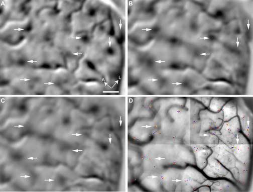
Co-localization of color patches and peak clusters. (A) A differential image that compares the response to red/green gratings with that to black/white gratings. The arrows point to some color patches that preferentially responded to chromatic gratings. (B)-(C) Single-condition images associated with uniform red and blue, respectively. (D) Peak locations marked on an anatomical image of the surface. The peak clusters pointed by the arrows correspond to those shown in Fig. 6E-L. The location of the arrows is fixed across different panels. A, anterior; L, lateral; Scale bar: 500 μm.
Image processing was carried out with MATLAB (MathWorks, MA) and ImageJ (National Institutes of Health, USA).
Results
Population response in V1 to uniformly colored stimuli
To visualize how the spatial distribution of neural activity in V1 depends on stimulus color, we imaged intrinsic optical signals across V1 in response to static, spatially uniform colors. In each experiment, nine to eleven photometrically isoluminant stimuli of different colors were used (Fig. 1). For each stimulus, we calculated a ‘single-condition’ image that represents the relative change in surface reflectance elicited by the stimulus. In these single-condition images, darker areas represent regions with stronger neuronal activation (Meister and Bonhoeffer, 2001; Tsunoda et al., 2001; Xiao et al., 2003).
Fig. 2 illustrates band-pass filtered single-condition images derived from an experiment in which stimuli were presented monocularly. Panels A-D show responses to red, yellow, green, and blue stimuli, respectively. To determine the reproducibility of the single-condition images, we presented the red stimulus twice in each imaging block, and derived two red-associated images from independent sets of raw data (panels A&E). Panel F is a single-condition image derived from control trials in which no stimulus was presented.
Fig. 2.

V1 responses to uniformly colored stimuli. (A)-(E) Single-condition images representing the spatial distribution of activities elicited by stimulation with red, yellow, green, blue, and a repeated red, respectively. The dark patches represent activated regions, except for the elongated ones along large blood vessels. The framed regions in panels A-D are enlarged and shown in Fig. 3. (F) A single-condition image derived from control trials in which no stimulus was presented. (G)-(H) Differential images calculated by subtracting panel E from panels A and D, respectively. A, anterior; L, lateral; ΔR/R, band-passed value of the relative change in surface reflectance. Scale bar: 500 μm.
Fig. 2 shows that each uniform color stimulus activated an array of patches that were about 200 μm wide at half height and were spaced more than 400 μm apart. These patches were not present in the control image (panel F). The patches activated by different colors were partially overlapping. The responses to end-spectral colors (red and blue, panels A and D) were stronger than those to mid-spectral colors (e.g., yellow and green, panels B and C). These results are all consistent with a previous study using 14C-2-deoxy-d-glucose (2DG) (Tootell et al., 1988b).
A comparison of panels A and E of Figure 2 shows that the spatial pattern of the response elicited by a given color was reproducible. To demonstrate this reproducibility more clearly, we derived a differential image (panel G) by subtracting panel E from panel A. There is no clear pattern in this differential image, suggesting that the patterns in panels A and E were similar and were canceled out by the subtraction. In contrast, the differential image (panel H) generated from panels D and E contains pairs of nearby bright (positive) and dark (negative) patches. The presence of these pairs of patches suggests that the response patches elicited by blue (panel D) and red (panel E) were displaced from each other by short distances.
Spatial organization of response patches associated with various colors
To further explore the dependence of the precise location of the activated patches on stimulus color, we first identified the significantly activated regions in response to each stimulus. A paired t-map was used to determine the statistical significance of the response of each pixel to a given stimulus. Within each paired t-map, we identified the regions activated by a given stimulus using a threshold of t that corresponds to a significance level of P<10−5 (one tail). Within each significant region, we then located the strongest responses by identifying the darkest pixel in a given single-condition image. The locations of these strongest responses are referred to below as the peak locations of the corresponding response patches.
Fig. 3 illustrates the two framed parts of the single-condition images shown in Fig. 2. Panels A-D and E-H of Fig. 3 correspond to the upper-right and lower-left frames, respectively. The peak location in each panel is marked by a white square. The cross in each panel marks the center of the panel. This figure shows that, although the patches activated by different colors partially overlapped, each patch peaked at a slightly different location.
Fig. 3.

Enlarged views of the framed regions in Fig. 2A-D. (A)-(D) The upper-right frame in panels A-D of Fig. 2, respectively. (E)-(H) The lower-left frame in panels A-D of Fig. 2, respectively. Each white square marks the peak location of a response patch. Cross: the center of each panel; Scale bar: 100 μm.
The partial overlap between differently activated patches is illustrated more clearly in Fig. 4, in which the contours of their peak region are superimposed. Each contour was drawn at the level of 75% of the maximal response of the corresponding patch, and was drawn with the color of the associated stimulus. Panels A and B represent the peak-contour maps in the upper and lower framed regions shown in Fig. 2, respectively. Due to the extensive overlap between different contours, it is hard to discern the order of the relatively small displacements among different peak response regions in these contour maps. To quantify these displacements, we concentrate our further analysis on the location of the maximal response in each patch, namely, the peak location. We have chosen the peak location rather than the centroid of the peak region (or other geometrical parameters) as the landmark of each response patch for several reasons that are given in the Discussion. However, the results based on the analysis of peak locations or centroids were similar.
Fig. 4.
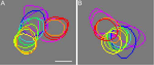
Contours of the peak response regions activated by different colors. (A) The contours derived from the region in the upper-right frame in Fig. 2. (B) The contours derived from the region in the lower-left frame in Fig. 2. The color of each contour corresponds to the color of the associated stimulus. Scale bar: 100 μm.
To examine the relationship between the peak locations associated with various colors, we marked each peak location with a square that has the color of the associated stimulus. Fig. 5A shows a map of peak locations overlaid on the anatomical image of the cortical surface. It demonstrates that the response peaks associated with various colors were clustered in small areas that were about 200 μm across. Neighboring clusters of these response peaks were spaced more than 400 μm apart. Because the optical signal is not spatially reliable near large blood vessels due to pulsations, the response peaks at or near large blood vessels were excluded from further analysis.
Panels B-G of Fig. 5 show a magnified view of peak clusters 1-6 labeled in panel A. The cluster shown in panel B consists of one response peak for each of the twelve stimuli, except for the orange stimulus and one of the two red stimuli, which gave rise to two peaks each. For the orange and red stimuli, the weaker peak of a pair is marked with a triangle of the appropriate color, and the stronger one is marked with a square. Our subsequent analysis is concentrated on the strongest peak, when multiple peaks associated with a stimulus are present in a peak cluster.
Relationship between stimulus colors associated with neighboring response peaks
In the cluster shown in Fig. 5B, each pair of closest peaks is associated with a pair of colors that have closest hues among the colors we tested, suggesting that spatial relationship among response peaks are related to the perceptual relationship among the associated colors. For instance, the peak associated with reddish purple is spatially closest to the one associated with purple, and the latter is next to the blue-associated peak. This hue-dependent proximity relationship also holds for the majority of response peaks in other clusters shown in Fig. 5, except for cluster 6 shown in panel G. The possible reason for the random organization of cluster 6 is given below (see section Reproducibility). In this and in the following analyses, we calculated the average position of the two red-associated peaks that were derived from independent data sets, and used that average as the location of the red-associated peak in a given cluster. Across all clusters analyzed in this study, the median distance between two red-associated peaks in each cluster was only 13.6 μm.
Across all peak clusters visualized in four animals, 79% of the response peaks (151 out of 190) followed the hue-dependent proximity relationship. Fig. 6 shows all clusters analyzed in this study, in addition to those already shown in Fig. 5. Each of these clusters is associated with at least seven different colors. In some clusters, one or more tested colors are not present because they did not elicit significant responses at the corresponding locations, or their peaks were near large blood vessels. For these clusters, a pair of colors that flanked the missing one was treated as having closest hues. For instance, yellow and green were regarded as the closest hue pair for the cluster shown in Fig. 6F, where a lime-associated peak is missing and the hue green-lime (GL) was not used in this experiment. This and further analyses were performed on all clusters associated with seven or more colors. The minimal number of seven was chosen as a compromise between the need to densely sample color space and the desire to have a large sample of clusters to analyze.
If each of the analyzed clusters were associated with only seven colors, and the response peaks were randomly located in each cluster, 33% of the response peaks would be expected to follow the hue-dependent proximity relationship by chance. The probability that 151 out of 190 (79%) response peaks will follow that relationship by chance is smaller than 10−40 (χ2 test). For a random cluster associated with more than seven colors, less than 33% of the response peaks would be expected to follow the hue-dependent proximity relationship, which further reduces the probability derived from the χ2 test. Therefore, our results suggest that the response peaks to various colors were not arranged randomly within each peak cluster, but instead followed the hue-dependent proximity relationship.
The peak clusters shown in Fig. 6 were visualized from four animals. Those in panels A-D were from the hemisphere shown in Fig. 2 and 5A (Case 4), but were obtained with binocular stimulation. They were not present in Fig. 5A, suggesting that they were driven by the eye that was closed during the experiment that generated Fig. 5A. Those in panels E-L, M-N, and O-P were from Cases 3, 2, and 1, respectively. Monocular stimulation was used in Cases 1 and 3, whereas binocular stimulation was used in Case 2.
Topological relationship within each cluster of response peaks
The hue-dependent proximity relationship describes the relationship between the associated stimulus colors for any pair of neighboring response peaks, and indicates a location-based representation of stimulus hue within each peak cluster. However, it does not tell us how the spatial organization of an entire peak cluster is related to the organization of the stimuli in color space. To address this global relationship, we performed another analysis. For each peak cluster, we connected all the peaks in such a way that the total physical length of the connecting line is the shortest among all possible connections. For instance, the shortest connection in Fig. 5B is K-R-O-RP-P-B-A-G-GL-L-Y. Except for the first three peaks (K-R-O), all the peaks along this shortest path followed the same order as did the hues of their associated stimuli. In order for the first three peaks to follow the order of their associated hues as well, we need to make three swaps between them: one between the pink and the red peaks, one between the newly positioned pink peak and the orange one, and one between the orange and red peaks. Thus, in this cluster, three swaps are needed in order to make all peaks along the shortest path follow the order of their associated hues. For a randomly arranged cluster with 11 peaks, the number of required swaps could be between 0 and 18. By calculating the number of needed swaps for each possible arrangement within a cluster that have 11 peaks, we found that the average number of needed swaps across a population of randomly arranged clusters is 13. Similarly, we calculated the average numbers of needed swaps for other categories of clusters, each consisting of a different number of peaks (from 7 to 10). To quantify the extent to which the order of all peaks in a given cluster deviated from the order of the associated hues, we used the number of swaps required for that cluster, divided by the average number of required swaps across randomly organized clusters of the corresponding category. We call this number the disorder index (DI). A cluster whose peaks are arranged strictly in the order of their associated hues has a DI of 0. For the cluster shown in Fig. 5B, the DI is 0.23 (3 divided by 13).
For the 22 clusters we studied, the average DI is 0.32 ± 0.05 (mean ± SEM.), which is much smaller than the value of 1.0 expected from a population of randomly arranged clusters. This small value of the average DI suggests that the majority of response peaks within each cluster were arranged on the cortex according to the hue order of their associated stimuli.
Fig. 7 shows the distribution of DI among the imaged clusters (black bars), compared with its distribution in a group of randomly organized clusters (gray bars). To compute the latter distribution, we first derived the probability function p(DI) for each category of randomly organized clusters. The category is defined by the number of peaks in each cluster. p(DI) was derived by calculating the DI for each possible arrangement of peaks in a cluster belonging to a given category. Each p(DI) was then multiplied by the number of imaged clusters that belonged to the corresponding category. For instance, we have imaged 6 clusters with 7 peaks each, so the p(DI) of this category (7 peaks/cluster) was multiplied by 6. Finally, these weighted p(DI) were summed to produce the predicted distribution of DI in a group of randomly organized clusters. Fig. 7 demonstrates that the number of imaged clusters that had small DIs was greater than that predicted from a group of randomly organized clusters. According to this predicted distribution, less than 20.7% of all clusters have a DI <0.8. Since the DI of each imaged cluster was smaller than 0.8, it is nearly impossible that they were all drawn from the population of randomly organized ones (P< 0.20722, or approximately 10−15). This result suggests that the observed preservation of hue order in most peak clusters has a biological origin. Furthermore, the analysis of DI and that of the similarity in associated hue between neighboring peaks both suggest that each peak cluster forms a location-based representation of stimulus hue, in which nearby locations represent perceptually similar hues.
Fig. 7.

Distribution of the Disorder Index (DI) in the imaged clusters (black bars) and in randomly-arranged clusters (gray bars). The two distributions are significantly different (P<10−15, see text).
The peak clusters had various geometrical shapes, even within a given hemisphere (e.g., Fig. 5). In addition, the two ends of the shortest path in a cluster varied among the various clusters. After a small number of swaps is made to bring the whole cluster into the order of hue (see above), the two ends are associated with perceptually similar hues in most clusters. The similarity in their associated hues between these two ends reflects the fact that a full gamut of hues constitutes a full cycle.
Regardless of its shape, an average cluster in this study was restricted to a small area of 162 ±10 μm long (mean ±SEM., n=22), as measured by the largest distance between any pair of peaks within each cluster.
Dependence of peak location on stimulus hue
Peak displacement is caused by a hue change, not variability
In an average peak cluster observed in this study, the response peaks associated with different stimuli were displaced from each other by no more than 162 μm. To establish that these displacements were not caused by the variability of the peak location associated with any stimulus, we need to compare them with the displacement between the pair of red-associated peaks that were derived from independent data sets. Fig. 8A plots the median distances from one of the red-associated peaks to other peaks, derived from 22 clusters. The asterisks denote distances that were significantly greater than the distance between the pair of red-associated peaks (P<0.0001, Mann-Whitney U test). The median distance between the pair of red-associated peaks was 13.6 μm (the interquartile range, or IQR, was 18.2 μm, n=19), suggesting a rather small variability of the peak location associated with a given stimulus. Relative to this red-to-red distance, the distance between red-associated peaks and each of the other peaks was significantly greater (P<0.0001), except for peaks associated with pink or orange, hues that are closest to red (in our stimulus set). This result suggests that the displacements between most pairs of response peaks were indeed caused by the difference in the hue of their associated stimuli.
Fig. 8.
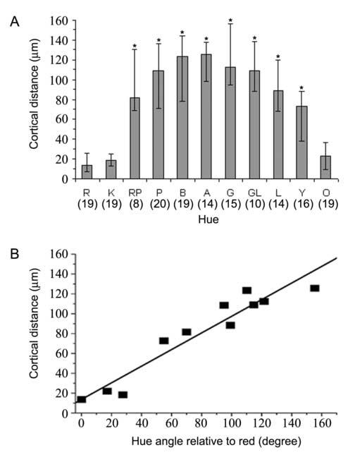
Cortical distances to a red-associated peak from other hue-specific peaks in each cluster. (A) The median distances displayed in the order of stimulus hue. Compared with the separation between two red-associated peaks in each cluster, the peaks associated with other hues were significantly more distant from a red-associated one, except for peaks associated with pink or orange. Error bar: IQR; *: P<10−4 , Man-Whitney U test, one tail, n is given under each hue. (B) The median distance as a function of the hue angle relative to the red. The straight line represents the linear regression between these hue difference and cortical distance. The correlation between these two variables is significant (r2=0.91, P<10−5). See Fig. 1 for color names abbreviations.
The reliability of the peak location associated with each stimulus color was further demonstrated in another experiment, in which each imaging block consisted of six trials with identical red stimuli, one trial with each of blue, green, and yellow stimuli, and two trials with red stimuli at different luminance levels. Panels A-C of Fig. 9 show three examples of the peak cluster visualized in this experiment. Compared with the separation between peaks associated with different colors, the majority of red-associated peaks were close to each other, except for those in Fig. 9C. In each of 15 clusters visualized in this experiment, we measured the distances from a randomly chosen red peak (called the reference peak below) to the other five red peaks. The median distance was only 12.2 μm (IQR = 7.5 μm, n=66), suggesting again that the variability in the peak location was too small to account for the displacement between most pairs of the differently-activated peaks.
Fig. 9.
Reproducibility of peak clusters and the effect of luminance. (A)-(C) Repeated imaging of the clusters shown in panels D-F, after five hours. Only four hues (red, yellow, green, blue) were used in this experiment, but the same red stimulus was repeated six times, producing six red-associated peaks in each cluster. In addition, a brighter red stimulus and a darker red one were also used, and their associated peaks are marked over two red squares by a white and black cross, respectively. (D)-(F) Re-drawn of the clusters shown in panels I, F, and L of Fig. 6, respectively. Scale bar: 100 μm.
Correlation between hue difference and cortical distance
To quantitatively assess the relationship between the physical peak displacement and the perceptual difference in hue of the associated stimuli, we plot the distance values presented in Fig. 8A as a function of the difference in hue angle between each stimulus color and red (Fig. 8B). The hue angle of each stimulus color, huv, is defined in the CIE 1976 (L*u*v*)-space (see Methods). The difference in hue angel between any pair of colors (|Δhuv|, or 360-|Δhuv| when |Δhuv| is greater than 180 degrees) is used to quantify their perceptual difference in hue. Fig. 8B shows that the cortical distance between response peaks is significantly correlated with the difference in hue between the associated stimulus color (r2 = 0.91, P < 10−5), when the red-associated peak is used as the reference point for perceptual comparisons. This result shows that the spatial organization of each peak cluster is not random with respect to the stimulus hue, and thus supports our earlier suggestion, that each peak cluster represents a possible hue map.
Effect of luminance
Although all stimuli tested were designed to have the same photometric luminance (9.5 cd/m2), there could be small luminance differences among these stimuli due to the difference in spectral sensitivity between different species, retinal eccentricities and individual animals (Jacobs and Deegan, 1997). To test the effect of luminance on the peak location, in the experiment associated with Fig. 9, we also included 2 trials using stimuli that had the same CIE coordinates as our standard red, but different luminance levels. The two non-standard reds had luminance of 19 cd/m2 and 4.5 cd/m2, respectively. In Fig. 9A-C, the peak locations associated with these bright and dim reds are marked by red squares under a white or black cross, respectively. It is clear from Fig. 9A-C that the luminance level had little effect on peak location. Across all visualized clusters, the distances from each of these two peaks to the reference red peak were not significantly different from the distance between the reference peak and the other five red peaks (P>0.1, Mann-Whitney U test, two-tails, n= 12 and 13 for the groups of reduced luminance and increased luminance, respectively, n=66 for the isoluminance group). In contrast, the peaks associated with three other colors were significantly separated from the reference red one (P<0.0001, Mann-Whitney U test, one-tail, n= 13, 9, 8 for blue, green, and yellow, respectively). These results rule out the possibility that the significant separation between peaks associated with different colors were caused by any spurious differences in luminance among our photometrically isoluminant stimuli. In addition, because spurious differences in luminance among various stimuli were likely random, it is unlikely that they could account for the observed arrangement of the response peaks that followed the hue order of the associated stimuli.
Reproducibility of peak clusters
The peak clusters shown in panels A-C of Fig. 9 were located in the same cortical regions as those shown in panels D-F, respectively. But these two sets of clusters were derived from two different experiments separated by 5.3 hours. Panels D-F are re-drawn of panels I, F and L of Fig. 6. A comparison of Fig. 9A-C with Fig. 9D-F establishes that the spatial arrangement of each cluster was reproducible across experiments separated by more than 5 hours. The reproducibility for the cluster shown in panels C&F was not as good as that for other clusters, probably due to the reason given in the next paragraph. For each pair of clusters derived from these two experiments, we measured the distance from each red peak derived from the first experiment to each red peak derived from the second one. The median value of this distance was 17.3 μm (IQR = 12.2 μm, n=174). Similarly calculated distances for blue, green, and yellow peaks were 18.3 μm (IQR = 29.7 μm, n=12), 40.9 μm (n=3), and 17.3 μm (IQR = 17.6 μm, n=7), respectively. These small distances suggest that most peak locations were highly reproducible across separate experiments, and were therefore reliable estimates of the location of their associated response patches. Since the variability in location of most peaks is small, as demonstrated by the above across-experiment and within-experiment analysis, it is unlikely to account for the variation in the geometrical shape of various clusters.
It is noteworthy that the two clusters shown in panels C and F of Fig. 9 were more different from each other compared with other pairs shown in the same figure. The poor reproducibility of peak location in this cluster was accompanied by the large separations between red-associated peaks that were derived from the same experiment (compare panel C with panels A and B). Coincidently, the full cluster shown in panel F appears to be randomly organized with respect to the hue order. It contained 44% of peaks that did not follow the hue-dependent proximity relationship, which was more than twice as great as the ratio (21%) across all clusters. It is likely that the random organization of this cluster was caused by the large variability in peak location at this part of the image. We noticed that the camera was focused at less than 100 μm below the cortical surface at this part of the image, whereas the majority of other clusters were derived from parts of images where the focal plane was 100-400 μm deep. The only two other clusters derived from the superficial focal plane (<100 μm) were those shown in Fig. 5G and 6K, which also had more than 42% of peaks that did not follow the hue-dependent proximity relationship. We speculate that small blood vessels at the cortical surface introduced greater noise at a superficial focal plane compared to deeper focal planes, which caused greater variability in peak location at the corresponding part of the image.
Monocular vs. Binocular stimulation
Monocular and binocular stimulations produced similar spatial organization of each peak cluster. The clusters shown in panels A-D of Fig. 10 were imaged at the same locations as those shown in panels E-H, respectively. They were derived from two experiments separated by 4 hours, one with binocular stimulation (A-D) and the other with monocular stimulation (E-H). Panels E-H are re-drawn of the clusters shown in Fig. 5B-D and G, respectively. The remaining two clusters in Fig. 5 are not displayed here because their binocularly-driven counterparts had only four peaks that were above the statistical threshold. The spatial organization of each cluster shown in Fig. 10 was similar under the monocular and binocular viewing conditions, except for the cluster shown in panels D and H. This similarity suggests that the monocularly-driven clusters that compose the major part of our data provide a good estimate of the corresponding peak clusters involved in normal, binocular viewing condition. The only irreproducible cluster in Fig. 10 (panels D and H) was one of the three clusters described above that were imaged at a superficial focal plane.
Fig. 10.

Binocular versus monocular stimulation. (A)-(D) Repeated imaging of the clusters shown in panels E-H, respectively, using binocular stimulation. (E)-(H) Re-drawn of the clusters shown in panels B, C, D, and G of Fig. 5, respectively. These clusters were visualized using monocular stimulation. Scale bar: 100 μm.
Hue maps and color patches
Previous studies have shown that V1 contains an array of regions that are preferentially activated by chromatic stimuli compared with achromatic stimuli (Orbach et al., 1996; Roe and Ts'o, 1999; Landisman and Ts'o, 2002a). These regions, called “color patches” by some investigators, have a higher concentration of color-selective cells than do the surrounding regions (Landisman and Ts'o, 2002a, b). To compare our study with these previous ones, we compared the V1 response to red/green gratings with that to black/white gratings in one animal (Case 3), using a set of stimuli that were similar to those used in the previous studies. The differential image derived from the above comparison in our study also contained an array of dark patches (Fig. 11A), which corresponded to the color patches described in previous studies. Examples of such patches are pointed by arrows in Fig. 11A.
Panels B and C of Fig. 11 illustrate single-condition images associated with spatially uniform red and blue stimuli, respectively, derived from the same area as that shown in panel A. Panel D illustrates the corresponding map of response peaks associated with all colors, overlaid on an anatomical image of the cortical surface. The arrows in panel D point to peak clusters illustrated in Fig. 6E-L. To facilitate comparison among four panels of Fig. 11, the arrows are located identically across these panels.
Panels A and B of Fig. 11 demonstrate that each patch activated by the uniform red was spatially registered with a color patch. Panel C shows that the blue-activated patches were also located near the color patches, but not as close to the latter as were the red-activated patches. The reduced proximity between the blue-activated patches and the color patches can be explained by the fact that the latter were visualized by using red/green and black/white gratings.
The median value of the distance between the red-associated peak in each analyzed peak cluster (pointed in Fig. 11D) and the peak of nearby color patch (pointed in Fig. 11A) was only 54.8 μm (IQR = 82.3 μm, n = 8). This result suggests that the peak clusters visualized in this study, or the hue maps, were co-localized with the color patches described in the previous studies. Because the color patches have a higher concentration of color-selective cells than do the surrounding regions (Landisman and Ts'o, 2002a, b), their co-localization with hue maps suggests that hue maps also contain relatively high concentration of color-selective cells. In addition, a previous study (Landisman and Ts'o, 2002a) found that the color patches have a high degree of overlap with CO blobs. Therefore the co-localization of these patches with the hue maps suggests the possibility that the hue maps also overlap with blobs extensively. This possibility is also supported by some of our preliminary results (Xiao et al., 2006).
Discussion
Hue maps in V1
We have found that stimuli of uniform color activated an array of patches (∼200 μm across) in the supragranular layers of parafoveal V1, and that the patches associated with different colors partially overlapped (Fig. 2-4). The peak locations of these activated patches were clustered in small cortical regions that are ∼160 μm long each (Fig. 5-6). Within each peak cluster, spatially close peaks were mostly associated with perceptually similar hues. The topological relationship among different peaks within each cluster largely followed the perceptual relationship among their associated hues. These results suggest that each peak cluster could represent a systematic hue map in which stimulus hue is coded by the location of response peaks. Each of these peak clusters represented a full gamut of hue, and different clusters often had different geometrical shapes.
In this study, we used static and spatially uniform stimuli. For a stimulus of this kind, its perceptual hue is determined completely by its coordinate in a colorimetrically-defined chromaticity space. Indeed, in the CIE 1976 (L*u*v*)-space, stimulus hue is specified by the angle of the line that connect the location of the stimulus in this space with that of the standard white (Wyszecki and Stiles, 1982). Our use of the term “hue” is qualitatively the same as that in the above CIE space. However, in a natural environment, the perceptual hue of a stimulus is not determined completely by its chromaticity coordinate (Wandell, 1995). Future experiments that use patterned stimuli are needed to address which of these two properties (perceptual hue or chromaticity coordinate) determines the peak location of the response.
The hue maps in V1 are similar to those we have previously discovered in the CO thin stripes of V2 (Xiao et al., 2003; Wang et al., 2006). However, the hue maps in V2 are 2.5 to 5 times as long as those in V1, consistent with the increase in the sizes of the color patches and orientation columns from V1 to V2 (Ts'o et al., 1990; Roe and Ts'o, 1995). Since hue maps in V1 may overlap extensively with blobs (see below), and blobs are more densely connected with the V2 thin stripes than are inter-blob regions (Livingstone and Hubel, 1984; Sincich and Horton, 2002; Xiao and Felleman, 2004; Sincich and Horton, 2005), it is likely that the hue maps in V1 and V2 are interconnected. Indeed, Roe and Ts'o (1999) have found hue-specific connectivity between neurons in V1 blobs and those in V2 thin stripes. However, how hue maps in one cortical area contribute to the formation of their counterparts in the other area remains to be determined.
Reliability of peak localization
Because at least 7 response peaks were confined within a small cortical area that is ∼162 μm long, high reliability in peak localization is critical for examining the spatial relationship among various peaks. To estimate the reliability of our measurements, we have included in each imaging block two separate trials that used identical red stimuli. Across all peak clusters, the median distance between two red-associated peaks was 13.6 μm. Similarly small variability of peak location was found in another experiment that included six repeats of the red stimulus. Thus the uncertainty in peak location is too small to account for the significantly greater distances that we found between red-associated peaks and peaks associated with most of the other colors (Fig. 8A).
Four main factors have contributed to the high reliability of our peak localization: 1) Each single-condition image was derived from at least 50 imaging trials, a relatively large number compared with previous studies that imaged intrinsic optical signals; 2) Our images were collected during the first 3.2 seconds following stimulus onset, when the intrinsic optical signal is more tightly correlated spatially with the local neural activity compared with the later period (Malonek and Grinvald, 1996); 3) We imaged the cortex at high resolution (6.1 μm/pixel), and then smoothed the single-condition images with a Gaussian filter that has a standard deviation of 7 pixels. The first part of this protocol enables us to discern small displacement between patches activated by different stimuli, while the second part reduces the variability in the value of each pixel caused by shot noise. When filters of smaller sigma were used on some images, the variability in the peak location was greater than that described above; 4) We concentrated our analysis on the activated patches where each pixel had a relatively high S/N ratio (> 4.71), as measured in the corresponding t-map.
The high reliability of peak locations is one of the reasons why we have chosen them, rather than the centroid of the peak region or other geometrical parameters as the landmark of each response patch. Across the peak clusters labeled in Fig. 5, the median distance between the pair of red-associated peaks was 13.6 μm (n=6), whereas the median distance between the corresponding centroids was 14.9 μm. The slightly larger variability of the centroids could be caused by the presence of large blood vessels in most peak regions. There are two more reasons why have focused our analysis on the peak locations. First, it has been shown that the intrinsic optical signal spreads beyond the focal point where neuronal firing rates increase in response to a stimulus (Das and Gilbert, 1997). This blood-related spreading is particularly broad in single-condition images (Frostig et al., 1990). It is possible that this spreading contributed to some of the peak regions, and thus affected the location of their centroids. On the other hand, the peak locations are likely the sources of the spreading, and represent the locations with increased firing rates. Second, the centroids depend on the choice of a threshold that defines the peak regions, whereas the peak locations are independent of any threshold.
A recent computational study found that the spatial blur, which is inherent in the imaging of intrinsic signal, can severely distort a vector-valued image (Polimeni et al., 2005). A vector-valued image, such as the orientation selectivity map, is derived from a vector summation of individual differential or single-condition images. However, as the authors of that study pointed out, the spatial blur has much smaller effect on a scalar-valued image compared with a vector-valued one. A scalar-valued image, such as a single-condition image, is a two-dimensional pattern of changes in surface reflectance. Since our analyses were focused on location of response peaks in each single-condition image, and did not involve any vector summation, our results should be relatively insensitive to the spatial blur. In addition, the blur is not likely to make a random cluster appear highly organized.
The small variability in peak location reported here represents an advantage of optical imaging over electrode recording for locating the peak response. Successive electrophysiological recordings from single units cannot locate the peak reliably, because only a very limited number of units can be recorded from each penetration, and the heterogeneity of neuronal population makes the comparison across penetrations unreliable. In addition, it is impractical to make more than 10 penetrations in a small range of 160 μm, which is required if one tries to confirm the spatial layout of a hue map with electrodes. Therefore, electrode recording cannot be used to either confirm or challenge our results directly. A potentially ideal tool for this task is in vivo calcium imaging with two-photon microscope, which has been used to image the spiking activity of a group of neurons in non-primate animals (Ohki et al., 2005).
Hue maps and CO blobs
The hue maps we have uncovered were co-localized with patches that were preferentially activated by chromatic gratings. These previously discovered color patches have been found to have a high degree of overlap with CO blobs (Landisman and Ts'o, 2002a). Therefore, the co-localization of these patches and hue maps suggests the possibility that the hue maps also overlap extensively with blobs. This possibility is supported by two additional lines of evidences presented below, as well as by some of our preliminary results (Xiao et al., 2006).
First, a study using the 2DG technique also found that spatially uniform color stimuli activated an array of V1 patches that were co-localized with CO blobs (Tootell et al., 1988b). These patches are likely to correspond to the patches visualized in our study because we also used spatially uniform stimuli. In both studies, the amplitude of the responses to end-spectral hues were stronger compared with those to mid-spectral hues.
Second, several studies have reported that, on average, cells inside CO blobs are tuned to lower spatial frequency compared with cells outside blobs (Tootell et al., 1988a; Born and Tootell, 1991; Edwards et al., 1995). Since our stimuli were all spatially uniform, these previous studies lead to the expectation that the response peaks in our study were located inside or near blobs.
Since it was first reported by Livingston and Hubel (1984) that CO blobs contain a higher concentration of color-selective cells and a lower concentration of orientation-selective cells compared with inter-blob regions, the question of whether blobs are specialized for processing color information has remained one of the central controversies regarding the functional organization of V1 (Livingstone and Hubel, 1988; Ts'o and Gilbert, 1988; Lennie et al., 1990; Leventhal et al., 1995; Yoshioka and Dow, 1996; Landisman and Ts'o, 2002a, b). We have preliminary results from one animal in which we stained the brain for CO (Xiao et al., 2006). The results from that animal showed a high degree (but not 100%) of overlap between CO blobs and hue maps, consistent with the arguments presented above. However, aligning functional images with CO-stained section precisely is extremely difficult at fine spatial scale, largely due to the problem of parallax and the distortion of the stained sections. Because of this well-known difficulty, our preliminary results can not provide a definitive answer to the question of whether each hue map is confined entirely within a CO blob. Addressing this important question may require new techniques that can visualize CO blobs in vivo.
Spatial arrangement of hue-selective cells
Several previous studies have found clusters of V1 cells that responded better to color than to luminance or patterned stimuli (Hubel and Wiesel, 1968; Dow and Gouras, 1973; Dow, 1974; Gouras, 1974; Michael, 1981; Livingstone and Hubel, 1984; Landisman and Ts'o, 2002a, b), and these observations are consistent with our results showing that an array of patches in V1 responds vigorously to color stimuli. However, only a few studies have addressed the spatial relationship between cells preferring various hues, and the results are inconsistent. One study found that V1 contains regions of ∼300 μm long where all cells preferred a specific hue (Michael, 1981). Two other studies reported that each blob contained either red/green cells or blue/yellow cells (Ts'o and Gilbert, 1988; Landisman and Ts'o, 2002b), and that the red/green blobs were three times as numerous as the blue/yellow blobs (Ts'o and Gilbert, 1988). These two studies are inconsistent with an earlier study that found red/green and blue/yellow cells in the same blobs (Livingstone and Hubel, 1984). Finally, another study found that most blob cells prefer end-spectral hues, while most interblob cells prefer mid-spectral ones (Yoshioka and Dow, 1996).
Our study focused on the peak location of the response patches to a given hue, rather than hue preference at each pixel. Because the responses to end-spectral hues were much stronger than those to the mid-spectral ones (Fig. 2) (Tootell et al., 1988b), the peak location associated with a mid-spectral hue often responded preferentially to an end-spectral hue. For instance, the peak location associated with yellow often responded more to blue than to yellow. This stronger optical response to an un-associated hue at a given peak location might either be caused by the spread of optical signal beyond the focal point where neuronal firing rate increased in response to the un-associated hue (Das and Gilbert, 1997), or indicates a mixture of cells preferring different hues at that peak location. Due to the above uncertainty, our results can not be taken as evidence for or against the fine-scale segregation of cells tuned to various hues. Extensive electrophysiological recordings from many neurons at each peak location are required to investigate this fine-scale segregation, which is beyond the scope of our paper.
However, the size of each hue map (∼160 μm) makes our result incompatible with the hypothesis that red/green and blue/yellow are represented in different sets of CO blobs ((Ts'o and Gilbert, 1988; Landisman and Ts'o, 2002b). More specifically, the average distance between red and blue peaks in a hue map was 124 μm (Fig. 8), much smaller than the distance between neighboring blobs (350-550 μm)(Horton, 1984). This small size of each hue map is compatible with the finding that a blob contains both red/green and blue/yellow cells (Livingstone and Hubel, 1984). Compared with the hypothesis of dual blob system (one for red/green, one for blue/yellow), the one of single blob system is more consistent with the anatomical findings that the supragranular layers of all blobs receive inputs from the konio-cellular layers of the LGN, which carry s-cone signals (Livingstone and Hubel, 1982; Fitzpatrick et al., 1983; Itaya et al., 1984; Hendry and Reid, 2000; Chatterjee and Callaway, 2003). In addition, the latter hypothesis is supported by a previous study using the 2DG technique, which showed that both red and blue stimuli activated the full set of CO blobs (Tootell et al., 1988b).
The advantage of peak-location-based representation of hue
Our findings of hue maps in V1 and V2 suggest that stimulus hue could be represented by the peak location of response patches elicited by a given stimulus. This peak-location-based code does not rely on the absolute amplitude of each responding column or neuron, but on a comparison among them. It is well established that the neural response to repeated presentations of a stimulus is variable (Schiller et al., 1976; Dean, 1981; Snowden et al., 1992; Croner et al., 1993), although the exact extent of this variability in V1 has been debated (Gur and Snodderly, 1997; Kara et al., 2000; Gur and Snodderly, 2006). If the variability of neighboring neurons is uncorrelated, the mean firing rate of neurons within a cortical column will be relatively constant in response to each presentation of a given stimulus (Britten et al., 1992). However, the variability of neurons located as far apart as 1 mm is usually correlated (Arieli et al., 1996), presumably due to ongoing cortical activity and intracortical connections. Because of this correlated variability, any coding scheme that depends on the absolute firing rate of each column will be unreliable. In contrast, a code that is based on peak location depends on both the averaging within each column and a comparison between them. The operations of averaging and comparing can minimize the uncorrelated and correlated variability, respectively.
Conclusions
Our results suggest that the primate V1 contains an array of hue maps, in which the hue of a spatially uniform stimulus is represented by the location of the peak response to the stimulus. Nearby locations in these maps represent perceptually similar hues. It remains to be determined whether the same set of hue maps also represents hue of patterned stimuli.
Acknowledgements
We thank Christopher Kavanau, Takeshi Yokoo, Jason Snell, Yao Chen, Tanya Nauvel, and Alex Beylin for their help with data analysis, programming and technical support. This research was supported by grants from NIH to E.K. (EY016371 and EY12867), a grant from Fight for Sight to Y.X., a core grant from the National Eye Institute to the Mount Sinai School of Medicine (EY001867), and an unrestricted grant from Research to Prevent Blindness, Inc to the Department of Ophthalmology, Mount Sinai School of Medicine.
Footnotes
Publisher's Disclaimer: This is a PDF file of an unedited manuscript that has been accepted for publication. As a service to our customers we are providing this early version of the manuscript. The manuscript will undergo copyediting, typesetting, and review of the resulting proof before it is published in its final citable form. Please note that during the production process errors may be discovered which could affect the content, and all legal disclaimers that apply to the journal pertain.
References
- Arieli A, Sterkin A, Grinvald A, Aertsen A. Dynamics of ongoing activity: explanation of the large variability in evoked cortical responses. Science. 1996;273:1868–1871. doi: 10.1126/science.273.5283.1868. [DOI] [PubMed] [Google Scholar]
- Blasdel GG, Salama G. Voltage-sensitive dyes reveal a modular organization in monkey striate cortex. Nature. 1986;321:579–585. doi: 10.1038/321579a0. [DOI] [PubMed] [Google Scholar]
- Born RT, Tootell RB. Spatial frequency tuning of single units in macaque supragranular striate cortex. Proceedings of the National Academy of Sciences of the United States of America. 1991;88:7066–7070. doi: 10.1073/pnas.88.16.7066. [DOI] [PMC free article] [PubMed] [Google Scholar]
- Britten KH, Shadlen MN, Newsome WT, Movshon JA. The analysis of visual motion: a comparison of neuronal and psychophysical performance. J Neurosci. 1992;12:4745–4765. doi: 10.1523/JNEUROSCI.12-12-04745.1992. [DOI] [PMC free article] [PubMed] [Google Scholar]
- Chatterjee S, Callaway EM. Parallel colour-opponent pathways to primary visual cortex. Nature. 2003;426:668–671. doi: 10.1038/nature02167. [DOI] [PubMed] [Google Scholar]
- Conway BR. Spatial structure of cone inputs to color cells in alert macaque primary visual cortex (V-1) J Neurosci. 2001;21:2768–2783. doi: 10.1523/JNEUROSCI.21-08-02768.2001. [DOI] [PMC free article] [PubMed] [Google Scholar]
- Croner LJ, Purpura K, Kaplan E. Response variability in retinal ganglion cells of primates. Proc Natl Acad Sci U S A. 1993;90:8128–8130. doi: 10.1073/pnas.90.17.8128. [DOI] [PMC free article] [PubMed] [Google Scholar]
- Das A, Gilbert CD. Distortions of visuotopic map match orientation singularities in primary visual cortex. Nature. 1997;387:594–598. doi: 10.1038/42461. [DOI] [PubMed] [Google Scholar]
- Dean AF. The variability of discharge of simple cells in the cat striate cortex. Exp Brain Res. 1981;44:437–440. doi: 10.1007/BF00238837. [DOI] [PubMed] [Google Scholar]
- Dow BM. Functional classes of cells and their laminar distribution in monkey visual cortex. J Neurophysiol. 1974;37:927–946. doi: 10.1152/jn.1974.37.5.927. [DOI] [PubMed] [Google Scholar]
- Dow BM, Gouras P. Color and spatial specificity of single units in Rhesus monkey foveal striate cortex. J Neurophysiol. 1973;36:79–100. doi: 10.1152/jn.1973.36.1.79. [DOI] [PubMed] [Google Scholar]
- Edwards DP, Purpura KP, Kaplan E. Contrast sensitivity and spatial frequency response of primate cortical neurons in and around the cytochrome oxidase blobs. Vision Research. 1995;35:1501–1523. doi: 10.1016/0042-6989(94)00253-i. [DOI] [PubMed] [Google Scholar]
- Fitzpatrick D, Itoh K, Diamond IT. The laminar organization of the lateral geniculate body and the striate cortex in the squirrel monkey (Saimiri sciureus) J Neurosci. 1983;3:673–702. doi: 10.1523/JNEUROSCI.03-04-00673.1983. [DOI] [PMC free article] [PubMed] [Google Scholar]
- Friedman HS, Zhou H, von der Heydt R. The coding of uniform colour figures in monkey visual cortex. J Physiol. 2003;548:593–613. doi: 10.1113/jphysiol.2002.033555. [DOI] [PMC free article] [PubMed] [Google Scholar]
- Frostig RD, Lieke EE, Ts'o DY, Grinvald A. Cortical functional architecture and local coupling between neuronal activity and the microcirculation revealed by in vivo high-resolution optical imaging of intrinsic signals. Proc Natl Acad Sci U S A. 1990;87:6082–6086. doi: 10.1073/pnas.87.16.6082. [DOI] [PMC free article] [PubMed] [Google Scholar]
- Gouras P. Opponent-colour cells in different layers of foveal striate cortex. J Physiol. 1974;238:583–602. doi: 10.1113/jphysiol.1974.sp010545. [DOI] [PMC free article] [PubMed] [Google Scholar]
- Gur M, Snodderly DM. Visual receptive fields of neurons in primary visual cortex (V1) move in space with the eye movements of fixation. Vision Res. 1997;37:257–265. doi: 10.1016/s0042-6989(96)00182-4. [DOI] [PubMed] [Google Scholar]
- Gur M, Snodderly DM. High response reliability of neurons in primary visual cortex (V1) of alert, trained monkeys. Cereb Cortex. 2006;16:888–895. doi: 10.1093/cercor/bhj032. [DOI] [PubMed] [Google Scholar]
- Hanazawa A, Komatsu H, Murakami I. Neural selectivity for hue and saturation of colour in the primary visual cortex of the monkey. Eur J Neurosci. 2000;12:1753–1763. doi: 10.1046/j.1460-9568.2000.00041.x. [DOI] [PubMed] [Google Scholar]
- Hendry SH, Reid RC. The koniocellular pathway in primate vision. Annu Rev Neurosci. 2000;23:127–153. doi: 10.1146/annurev.neuro.23.1.127. [DOI] [PubMed] [Google Scholar]
- Horton JC. Cytochrome oxidase patches: a new cytoarchitectonic feature of monkey visual cortex. Philosophical Transactions of the Royal Society of London - Series B: Biological Sciences. 1984;304:199–253. doi: 10.1098/rstb.1984.0021. [DOI] [PubMed] [Google Scholar]
- Hubel DH, Wiesel TN. Receptive fields and functional architecture of monkey striate cortex. Journal of Physiology. 1968;195:215–243. doi: 10.1113/jphysiol.1968.sp008455. [DOI] [PMC free article] [PubMed] [Google Scholar]
- Itaya SK, Itaya PW, Van Hoesen GW. Intracortical termination of the retinogeniculo-striate pathway studied with transsynaptic tracer (wheat germ agglutinin-horseradish peroxidase) and cytochrome oxidase staining in the macaque monkey. Brain Res. 1984;304:303–310. doi: 10.1016/0006-8993(84)90334-2. [DOI] [PubMed] [Google Scholar]
- Jacobs GH, Deegan JF., 2nd Spectral sensitivity of macaque monkeys measured with ERG flicker photometry. Vis Neurosci. 1997;14:921–928. doi: 10.1017/s0952523800011639. [DOI] [PubMed] [Google Scholar]
- Johnson EN, Hawken MJ, Shapley R. The spatial transformation of color in the primary visual cortex of the macaque monkey. Nat Neurosci. 2001;4:409–416. doi: 10.1038/86061. [DOI] [PubMed] [Google Scholar]
- Kara P, Reinagel P, Reid RC. Low response variability in simultaneously recorded retinal, thalamic, and cortical neurons. Neuron. 2000;27:635–646. doi: 10.1016/s0896-6273(00)00072-6. [DOI] [PubMed] [Google Scholar]
- Landisman CE, Ts'o DY. Color processing in macaque striate cortex: relationships to ocular dominance, cytochrome oxidase, and orientation. J Neurophysiol. 2002a;87:3126–3137. doi: 10.1152/jn.2002.87.6.3126. [DOI] [PubMed] [Google Scholar]
- Landisman CE, Ts'o DY. Color processing in macaque striate cortex: electrophysiological properties. J Neurophysiol. 2002b;87:3138–3151. doi: 10.1152/jn.00957.1999. [DOI] [PubMed] [Google Scholar]
- Lennie P, Movshon JA. Coding of color and form in the geniculostriate visual pathway (invited review) J Opt Soc Am A Opt Image Sci Vis. 2005;22:2013–2033. doi: 10.1364/josaa.22.002013. [DOI] [PubMed] [Google Scholar]
- Lennie P, Krauskopf J, Sclar G. Chromatic mechanisms in striate cortex of macaque. J Neurosci. 1990;10:649–669. doi: 10.1523/JNEUROSCI.10-02-00649.1990. [DOI] [PMC free article] [PubMed] [Google Scholar]
- Leventhal AG, Thompson KG, Liu D, Zhou Y, Ault SJ. Concomitant sensitivity to orientation, direction, and color of cells in layers 2, 3, and 4 of monkey striate cortex. Journal of Neuroscience. 1995;15:1808–1818. doi: 10.1523/JNEUROSCI.15-03-01808.1995. [DOI] [PMC free article] [PubMed] [Google Scholar]
- Livingstone M, Hubel D. Segregation of form, color, movement, and depth: anatomy, physiology, and perception. Science. 1988;240:740–749. doi: 10.1126/science.3283936. [DOI] [PubMed] [Google Scholar]
- Livingstone MS, Hubel DH. Thalamic inputs to cytochrome oxidase-rich regions in monkey visual cortex. Proceedings of the National Academy of Sciences of the United States of America. 1982;79:6098–6101. doi: 10.1073/pnas.79.19.6098. [DOI] [PMC free article] [PubMed] [Google Scholar]
- Livingstone MS, Hubel DH. Anatomy and physiology of a color system in the primate visual cortex. Journal of Neuroscience. 1984;4:309–356. doi: 10.1523/JNEUROSCI.04-01-00309.1984. [DOI] [PMC free article] [PubMed] [Google Scholar]
- Malonek D, Grinvald A. Interactions between electrical activity and cortical microcirculation revealed by imaging spectroscopy: implications for functional brain mapping. Science. 1996;272:551–554. doi: 10.1126/science.272.5261.551. [DOI] [PubMed] [Google Scholar]
- Meister M, Bonhoeffer T. Tuning and topography in an odor map on the rat olfactory bulb. J Neurosci. 2001;21:1351–1360. doi: 10.1523/JNEUROSCI.21-04-01351.2001. [DOI] [PMC free article] [PubMed] [Google Scholar]
- Michael CR. Columnar organization of color cells in monkey's striate cortex. Journal of Neurophysiology. 1981;46:587–604. doi: 10.1152/jn.1981.46.3.587. [DOI] [PubMed] [Google Scholar]
- Ohki K, Chung S, Ch'ng YH, Kara P, Reid RC. Functional imaging with cellular resolution reveals precise micro-architecture in visual cortex. Nature. 2005;433:597–603. doi: 10.1038/nature03274. [DOI] [PubMed] [Google Scholar]
- Orbach D, Everson R, Kaplan E. Color and Luminance processing in macaque V1: Spatial structure revealed by intrinsic optical imaging. Soc. Neurosci. Abstr. 1996;22:376.374. [Google Scholar]
- Polimeni JR, Granquist-Fraser D, Wood RJ, Schwartz EL. Physical limits to spatial resolution of optical recording: clarifying the spatial structure of cortical hypercolumns. Proc Natl Acad Sci U S A. 2005;102:4158–4163. doi: 10.1073/pnas.0500291102. [DOI] [PMC free article] [PubMed] [Google Scholar]
- Ratzlaff EH, Grinvald A. A tandem-lens epifluorescence macroscope: hundredfold brightness advantage for wide-field imaging. J Neurosci Methods. 1991;36:127–137. doi: 10.1016/0165-0270(91)90038-2. [DOI] [PubMed] [Google Scholar]
- Roe AW, Ts'o DY. Visual topography in primate V2: multiple representation across functional stripes. Journal of Neuroscience. 1995;15:3689–3715. doi: 10.1523/JNEUROSCI.15-05-03689.1995. [DOI] [PMC free article] [PubMed] [Google Scholar]
- Roe AW, Ts'o DY. Specificity of color connectivity between primate V1 and V2. J Neurophysiol. 1999;82:2719–2730. doi: 10.1152/jn.1999.82.5.2719. [DOI] [PubMed] [Google Scholar]
- Schiller PH, Finlay BL, Volman SF. Short-term response variability of monkey striate neurons. Brain Res. 1976;105:347–349. doi: 10.1016/0006-8993(76)90432-7. [DOI] [PubMed] [Google Scholar]
- Shapley R, Hawken M. Neural mechanisms for color perception in the primary visual cortex. Curr Opin Neurobiol. 2002;12:426–432. doi: 10.1016/s0959-4388(02)00349-5. [DOI] [PubMed] [Google Scholar]
- Sincich LC, Horton JC. Divided by cytochrome oxidase: a map of the projections from v1 to v2 in macaques. Science. 2002;295:1734–1737. doi: 10.1126/science.1067902. [DOI] [PubMed] [Google Scholar]
- Sincich LC, Horton JC. Input to V2 thin stripes arises from V1 cytochrome oxidase patches. J Neurosci. 2005;25:10087–10093. doi: 10.1523/JNEUROSCI.3313-05.2005. [DOI] [PMC free article] [PubMed] [Google Scholar]
- Snowden RJ, Treue S, Andersen RA. The response of neurons in areas V1 and MT of the alert rhesus monkey to moving random dot patterns. Exp Brain Res. 1992;88:389–400. doi: 10.1007/BF02259114. [DOI] [PubMed] [Google Scholar]
- Tootell RB, Silverman MS, Hamilton SL, Switkes E, De Valois RL. Functional anatomy of macaque striate cortex. V. Spatial frequency. Journal of Neuroscience. 1988a;8:1610–1624. doi: 10.1523/JNEUROSCI.08-05-01610.1988. [DOI] [PMC free article] [PubMed] [Google Scholar]
- Tootell RB, Silverman MS, Hamilton SL, De Valois RL, Switkes E. Functional anatomy of macaque striate cortex. III. Color. Journal of Neuroscience. 1988b;8:1569–1593. doi: 10.1523/JNEUROSCI.08-05-01569.1988. [DOI] [PMC free article] [PubMed] [Google Scholar]
- Ts'o DY, Gilbert CD. The organization of chromatic and spatial interactions in the primate striate cortex. Journal of Neuroscience. 1988;8:1712–1727. doi: 10.1523/JNEUROSCI.08-05-01712.1988. [DOI] [PMC free article] [PubMed] [Google Scholar]
- Ts'o DY, Frostig RD, Lieke EE, Grinvald A. Functional organization of primate visual cortex revealed by high resolution optical imaging. Science. 1990;249:417–420. doi: 10.1126/science.2165630. [DOI] [PubMed] [Google Scholar]
- Tsunoda K, Yamane Y, Nishizaki M, Tanifuji M. Complex objects are represented in macaque inferotemporal cortex by the combination of feature columns. Nat Neurosci. 2001;4:832–838. doi: 10.1038/90547. [DOI] [PubMed] [Google Scholar]
- Wachtler T, Sejnowski TJ, Albright TD. Representation of color stimuli in awake macaque primary visual cortex. Neuron. 2003;37:681–691. doi: 10.1016/s0896-6273(03)00035-7. [DOI] [PMC free article] [PubMed] [Google Scholar]
- Wandell BA. Foundations of Vision. Sinauer Associates, Inc.; Sunderland, MA: 1995. [Google Scholar]
- Wang Y, Xiao Y, Felleman DJ. V2 Thin Stripes Contain Spatially Organized Representations of Achromatic Luminance Change. Cereb Cortex Advance. 2006 doi: 10.1093/cercor/bhj131. Access published February 8, 2006. [DOI] [PubMed] [Google Scholar]
- Wyszecki G, Stiles WS. Color Science. 2nd Edition Jonh Wiley & Sons; New York: 1982. [Google Scholar]
- Xiao Y, Felleman DJ. Projections from primary visual cortex to cytochrome oxidase thin stripes and interstripes of macaque visual area 2. Proc Natl Acad Sci U S A. 2004;101:7147–7151. doi: 10.1073/pnas.0402052101. [DOI] [PMC free article] [PubMed] [Google Scholar]
- Xiao Y, Wang Y, Felleman DJ. A spatially organized representation of colour in macaque cortical area V2. Nature. 2003;421:535–539. doi: 10.1038/nature01372. [DOI] [PubMed] [Google Scholar]
- Xiao Y, Casti ARR, Xiao J, Kaplan E. A spatially organised representation of colour in macaque primary visual cortex. Perception. 2006;35(supplement):21. [Google Scholar]
- Yoshioka T, Dow BM. Color, orientation and cytochrome oxidase reactivity in areas V1, V2 and V4 of macaque monkey visual cortex. Behavioural Brain Research. 1996;76:71–88. doi: 10.1016/0166-4328(95)00184-0. [DOI] [PubMed] [Google Scholar]