Abstract
Longitudinal samples of DNA sequences, the DNA sequences sampled from the same population at different time points, have increasingly been used to study the evolutionary process of fast-evolving organisms, e.g., RNA virus, in recent years. We propose in this article several methods for testing genetical isochronism or detecting significant genetical heterochronism in this type of sample. These methods can be used to determine the necessary sample size and sampling interval in experimental design or to combine genetically isochronic samples for better data analysis. We investigate the properties of these test statistics, including their powers of detecting heterochronism, assuming different evolutionary processes using simulation. The possible choices and usages of these test statistics are discussed.
LONGITUDINAL samples, or serial samples, are samples taken at a series of time points from the same population. Strictly speaking, almost all DNA sequence samples in population genetics studies are longitudinal samples, since the sequence sample from different individuals is most likely taken at different times, although the time interval between samplings may be small. In most cases, such samples can be safely regarded as a sample taken at a single time point, which simplifies analysis of the data. The justification of such a convention is that the sampling interval is so small that the possible mutations accumulated on the sequences studied within the sampling intervals are negligible. In other words, these samples are genetically isochronic. However, for organisms with a very high mutation rate, e.g., RNA virus, caution must be taken in the sampling intervals because the genetic change within the samples may be significant. In fact, for fast-evolving organisms, samples are purposely taken at different time points to keep track of the change in the population. Several new statistical methods have been developed for analyzing longitudinal DNA samples (reviewed by Drummond et al. 2003).
Important questions with regard to the experimental design include how large a sample size and how long a sampling interval is needed for conducting a meaningful genetic analysis. Sample sizes that are too small may render the study useless and sampling intervals that are too long may lead to loss of important information from the population. Furthermore, very short sampling intervals may be unnecessary and cost ineffective.
Because genetic difference is the primary information in such studies, genetical isochronism is a suitable criterion for guiding experiment design. A test of genetical isochronism along with simulation can show the probability of detecting the desired genetic change within samples with given sample sizes, sampling intervals, and evolutionary models. Such tests can also be used to guide the combination of genetically isochronic samples to obtain a larger “single sample” in the data analysis. The increased sample size and reduced parameter space will in general lead to more powerful analysis.
Seo et al. (2002b) studied the optimal experimental design specially for estimating mutation rate and divergence time using longitudinal samples. The purpose of the present article is to develop general statistical tests for detecting genetical heterochronism (i.e., deviation from genetical isochronism). Assuming a fixed genealogy of the samples, such a test can be built under a likelihood framework (e.g., Rambaut 2000; Drummond et al. 2001; Rodrigo et al. 2003). However, the genealogy of the samples is usually unknown and not easy to infer with accuracy, so that a general test based on summary statistics without assumption of genealogies may be desirable. The tests proposed in this article are based on two groups of summary statistics of longitudinal samples, one of which is the average nucleotide difference between two sequences between and within samples, and the other is the number of private mutations within samples. Different linear combinations of these summary statistics were used to construct test statistics. Besides the permutation approach we also used simulation to determine the critical values of the tests. For each combination of test statistics and critical values, the test powers with different sample sizes and sampling intervals under different evolutionary models were investigated. Finally, the choices of test statistics and critical values under different circumstances are discussed.
CONSTRUCTING STATISTICAL TESTS
Genetical isochronism:
Define genetical isochronism as the genetic equivalence of two statuses of the same population at two successive time points, which is due to the time interval being relatively small such that the gene frequencies were not changed significantly by mutation and/or genetic drift, so that genetical isochronism is a statistical concept. If the two statuses of the population are significantly different, they are genetically heterochronic. Let G be a measure of the difference of gene frequencies between two samples taken at different time points in a population; then the null hypothesis of the test of isochronism is G = 0 and the alternative hypothesis is G > 0.
Two-sample model:
Suppose there are two samples taken from an evolving haploid population at times t0 and t0 + t, respectively, where t is the sampling interval in generations. Let n1 and n2 be the sizes of samples taken at t0 and t0 + t, respectively. Define the population mutation rate θ = 2Neμ, where Ne is the effective population size and μ is the mutation rate per gene site per generation, both assumed to be constant.
Test statistics based on the average nucleotide difference between two sequences between and within samples:
Let Πi (i = 1, 2) be the average number of nucleotide differences between two sequences from sample i. Let Π12 be the average nucleotide differences between two sequences, one from sample 1 and the other from sample 2. That is,
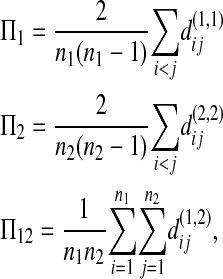 |
where  is the nucleotide difference between the ith sequence of sample k and the jth sequence of sample l.
The expectations of Π1, Π2, and Π12 under the neutral Wright–Fisher model are
 |
 |
 |
where E( ) stands for mathematical expectation (e.g. Drummond and Rodrigo 2000; Fu 2001).
Here testing genetical isochronism is equivalent to testing the null hypothesis of μt = 0. It is easy to see that the expectations of both (Π12 − Π1) and (Π12 − Π2) are equal to μt and that the expectations of any linear combination of (Π12 − Π1) and (Π12 − Π2) are equal to 0 under the null hypothesis. The above analyses result in the following form of test statistics by standardizing a linear combination of (Π12 − Π1) and (Π12 − Π2),
 |
(1) |
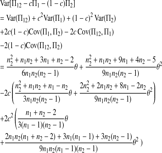
where
 |
(2) |
is the variance of  under the null hypothesis of μt = 0 (see appendix a).
Three particular values of c, 1, 0, and  are of interest. The first two correspond to
  and
and 
Since the expectation of  equals μt, a significant positive value of Dc is taken as evidence of heterochronism, which corresponds to the one-tail test of the alternative hypothesis of Dc > 0 vs. Dc = 0.
Test statistics based on the number of private mutations within samples:
Define the number of private mutations within a sample as the number of sites that are only polymorphic in that sample but are monomorphic in the other sample. Let Kp(i) (i = 1, 2) be the number of private mutations of sample i. Wakeley and Hey (1997) showed that the expectations of Kp(1) and Kp(2) under the null hypothesis are
 |
(3) |
 |
(4) |
where 
If the sampling interval is big, both samples will tend to contain more mutations that are “private” to that sample. In other words, the expectations of both Kp(1) and Kp(2) will be larger than their expectations under the null hypothesis of no sampling interval. So both Kp(1) and Kp(2) and their linear combinations can be used to test genetical isochronism. Therefore we consider a group of tests of the form
 |
(5) |
Five particular values of c, 1, 0, 0.5,  and
and  are of interest.
For example, if c = 1 or 0, (5) is simplified to  or
or 
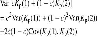
 is the variance of
  under the null hypothesis. There is no simple formula for
  However, it can be calculated with the formulas
 |
(6) |
 |
(7) |
 |
(8) |
 |
(9) |
 |
(10) |
 |
(11) |
 |
(12) |
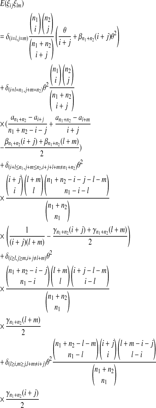 |
(13) |
 |
(14) |
 |
(15) |
where  is the number of mutations whose frequency is i in sample 1 and j in sample 2, and δ is an index variable such that it takes the value 1 if conditions in parentheses are true and takes the value 0 otherwise [see appendix b for derivation of (13)]. The test of genetical isochronism is equivalent to the one-tail test of the alternative hypothesis of Tc > 0 vs. Tc = 0.
DETERMINING THE LEVEL OF SIGNIFICANCE
Simulation:
Although all the test statistics proposed in this article are in standardized form, their distributions do not follow a normal distribution or other standard distributions under the null hypothesis, which is similar to the tests for single sample (e.g., see Fu and Li 1999). Furthermore, when such statistics are applied, an estimation of θ is needed to replace θ in formulas (2), (3), (4), and (13). Therefore simulation has to be used to determine the critical values of these tests. However, the standardization does help to minimize the effect of θ, n1, and n2 on the test statistics and will lead to more accurate and stable estimation of critical values using interpolation (see below).
To obtain the critical values of Dc's and Tc's, we first simulated independent samples under the null hypothesis with a large number of combinations of θ, n1, and n2. We chose 40 different n1 [n1 = 5 (5) 100 (10) 300, i.e., 5, 10, 15, …, 100, 110, …, 300], 40 different n2 [n2 = 5 (5) 100 (10) 300] and 46 different θ [θ = 0.2 (0.1) 1 (0.2) 3 (0.5) 4 (1) 20 (5) 50 (10) 80]. For each of the parameter sets, 20,000 independent samples were simulated using the coalescent algorithms (e.g., Hudson 1983). From each sample, all test statistics were calculated with θ's in formulas (2), (3), (4), and (13) replaced by Watterson's estimator (Watterson 1975)  where K is the total number of polymorphic sites when combining samples 1 and 2. The empirical critical values for each parameter set can be easily determined from the empirical distribution. For example, the critical value of a given test with a 5% significance level is the 95th percentile of the empirical distribution of that test statistic after ascending sorting. The critical values of other combinations of parameters can be obtained by interpolating the values from the big table obtained above.
Permutation:
Permutation or shuffling has been widely used in data analysis for conducting tests without assumption of normality of the test statistics (e.g., Ewens and Grant 2005). The procedure of permutation is easy to conduct: (1) combine sample 1 and sample 2 into a big sample; (2) randomly pick n1 sequences from the big sample to form a pseudosample 1 and let the remaining n2 sequences be pseudosample 2 (each one of such a shuffle is called a permutation); (3) from pseudosamples 1 and 2, calculate some specified test statistics; (4) repeat the process above from step 2 for a large number of times (20,000 times in our tests); and (5) the empirical critical values can be obtained similar to that of simulation.
The rationale behind the procedure is as follows. In the procedure of permutation, each test statistic estimated from each permutation has the same probability. If the null hypothesis is true, the actual observed value of the test statistic should have only probability α to be among the 100α% most extreme values. On the other hand, if the alternative hypothesis is true, the random permutation will tend to shift the distribution of the test statistic estimated from each permutation to that expected under the null hypothesis, which will make the actual observed value of the test statistic more likely to be among the extreme values.
POWERS OF THE TESTS
Since the main purpose of this research is to develop guidelines for experimental design, we are mostly interested in the effects of n1, n2, θ, and μt on the power of the tests. For each combination of parameters, 5000 independent samples were simulated using coalescent algorithms, which assume a neutral Wright–Fisher model with constant population size. Each test was applied to the simulated samples and the frequency of successful detections by a given test was used as an estimate of its power.
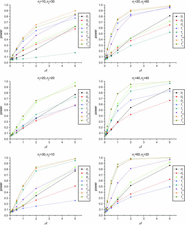
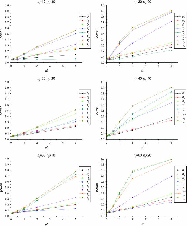
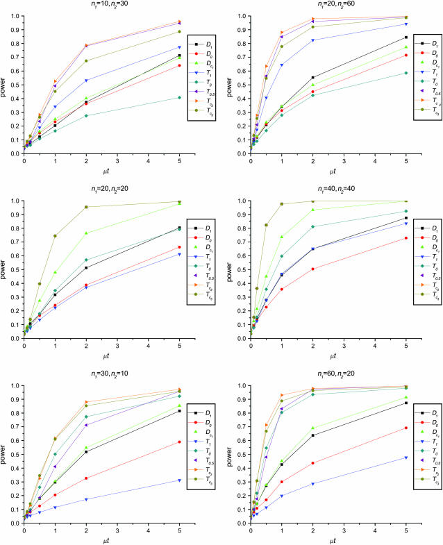
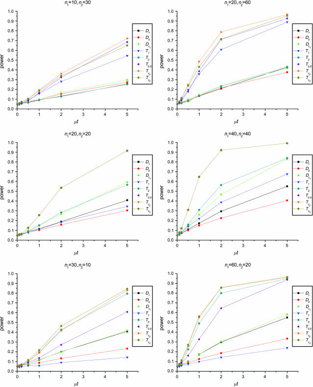
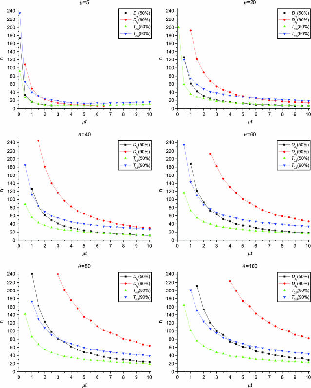
Figure 1 shows the powers of the tests (Dc's and Tc's) using the critical values determined by simulation, with different n1, n2, and μt and fixed θ = 10. Figure 2 shows the powers of the same tests with θ = 40. Figures 3 and 4 show the powers of the tests using the critical values determined by permutation, corresponding to the same parameters of Figures 1 and 2, respectively. Figure 5 shows the minimum sample sizes (assuming n1 = n2) needed to achieve 50 or 90% power using  and
and  (which are identical to
  and
and  in this case) with a 5% significance level. For example, to achieve 50% detection power using
  with a 5% significance level, we need a minimum sample size n1 = n2 = 16 for a population with θ = 5 or n1 = n2 = 101 for a population with θ = 100.
Figure 1.—
Powers of Dc's and Tc's with 5% significance level determined by simulation (θ = 10). T0.5,  and
and  are identical when n1 = n2.
Figure 2.—
Powers of Dc's and Tc's with 5% significance level determined by simulation (θ = 40). T0.5,  and
and  are identical when n1 = n2.
Figure 3.—
Powers of Dc's and Tc's with 5% significance level determined by permutation (θ = 10). T0.5,  and
and  are identical when n1 = n2.
Figure 4.—
Powers of Dc's and Tc's with 5% significance level determined by permutation (θ = 40). T0.5,  and
and  are identical when n1 = n2.
Figure 5.—
Minimum sample sizes, assuming n1 = n2
= n, needed to achieve 50 or 90% power using  and T0.5 (T0.5,
  and
and  are identical when n1 = n2) with 5% significance level.
The results can be summarized as follows:
The test power is positively correlated with μt, that is, the larger the μt the higher the power. On the other hand, θ is negatively correlated with the test power, i.e., the larger the θ the lower the test power.
The larger the total sample size the higher the test power, which is true for all test statistics. However, the effects of n1 and n2 on different test statistics are quite different. If total sample size is fixed, T0 and D1 have higher powers when n1 > n2 than when n2 > n1. On the contrary, T1 and D0 have higher powers when n1 < n2 than when n2 < n1. D1 and D0 have higher powers when n1 = n2 than when n1 > n2 or when n1 < n2.
 has higher power than T1 and T0 when n1 = n2, but its power is in between those of T1 and T0 when n2 > n1 or n2 < n1. The powers of
  and
and  are consistently better than those of both T1 and T0. The power
  is higher than that of D1 and D0 in general.
 and
and  are the most powerful test statistics in general.
  is also quite powerful when n1 = n2. Especially when μt is relatively large, e.g., the quantity is comparable to θ, it can be the most powerful test statistic under such a condition.
In general, tests using critical values determined by permutation are slightly more powerful than those using the critical values determined by simulation. This is largely because they consider the sampling variation but not the evolutionary variation (see discussion). But there are some exceptions; e.g., T1 may be slightly less powerful using the critical values from permutation rather than using those from simulation, especially when n1 < n2 and/or with population growth (see discussion).
AN EXAMPLE
Here we use longitudinal samples of env genes of human immunodeficiency virus (HIV)-1 from Rodrigo et al. (1999) to illustrate the use of the tests developed in this article. These longitudinal samples were taken from an AIDS patient over a course of 3 years. After the first blood sample was taken from the patient, four other blood samples were taken 7, 22, 23, and 34 months later. From each blood sample, between 8 and 15 DNA sequences of a 0.65-kb region of HIV env gene were obtained. The summary of their sample is listed in Table 1 of Rodrigo et al. (1999).
TABLE 1.
The values and P-values of test statistics for sample 1 vs. sample 2
| Test statistic | D1 | D0 |  |
T1 | T0 | T0.5 |  |
 |
|---|---|---|---|---|---|---|---|---|
| Value | 0.321 | 0.392 | 0.729 | 1.866 | 1.091 | 2.107 | 2.151 | 2.183 |
| P-value | 0.260 | 0.231 | 0.122 | 0.044 | 0.100 | 0.025 | 0.023 | 0.021 |
| 0.196 | 0.158 | 0.008 | 0.076 | 0.422 | 0.001 | 0.001 | 0.003 |
The first and second rows of P-values are determined by simulation and permutation, respectively.
Consider sample 1 and sample 2 first. We have 


 and
and  Then we obtained
  which replaces θ in formulas (2), (3), (4), and (13), and calculated the test statistics (Table 1). Finally, we used permutation and simulation to get the empirical distributions of the test statistics and then obtained the empirical P-values (Table 1).
Table 2 shows the P-values of  using the critical values determined by simulation and permutation for all pairwise comparisons of the samples. Most of them are <0.05, and therefore most pairs of samples can be regarded as significant deviation from genetical isochronism. However, all tests involving sample 5 based on simulation are not significant while all those based on permutation are significant or marginally significant. This may be due to the fact that the sample size of sample 5 is only eight and is the smallest one of all. With such a small sample size,
  based on simulation may be just lack of enough power as that based on permutation. This may be compounded by the possibility that the mutation rate changed after the third sampling time because of drug treatment (Drummond
et al. 2001).
TABLE 2.
P-values of Tc2 for pairwise comparisons of samples
| Sample | 1 | 2 | 3 | 4 | 5 |
|---|---|---|---|---|---|
| 1 | 0.023 | 0.008 | 0.003 | 0.060 | |
| 2 | 0.001 | 0.019 | 0.037 | 0.058 | |
| 3 | <0.001 | <0.001 | 0.045 | 0.084 | |
| 4 | 0.004 | 0.001 | 0.005 | 0.187 | |
| 5 | 0.049 | 0.010 | 0.019 | 0.027 |
P-values on the top diagonal and on the bottom diagonal are determined by simulation and permutation, respectively.
This example reveals the issues of sample size in experimental design. If one wants to study the evolution of HIV via longitudinal samples of env genes, the sampling interval of 1 year with sample size ∼20 is sufficient for a relatively conservative design.
DISCUSSION
In this article we proposed and studied two forms of test statistics for testing genetical isochronism, using critical values based on two different approaches, simulation and permutation. We showed that the tests with critical values determined by permutation are slightly more powerful than those determined by simulation. The permutation approach also has other advantages: no parameters need to be estimated (indeed no standardization is needed), and it is relatively fast for a small number of tests and easy to program. However, caution must be taken when using the permutation approach. There are two levels of variation in samples that will affect statistical tests. One level is due to the stochastic nature of evolution, that is, the variation of different replications (i.e., the resulting populations) of the same evolution process. The second level is due to the sampling process, that is, the variation of different samples from the same population. The permutation approach effectively assumes that the two samples are taken from the same population, thus taking into consideration only the second level of variation. The result is that the variances of test statistics are smaller than those from the simulation approach. Nevertheless, it provides the lower bound of the total variance. On the other hand, simulation considers both levels of variation, which makes it more conservative than permutation. Because of these differences, both approaches are useful. We suggest using critical values from simulation as the standard for experimental design, in which the evolution process is the subject of research. As to the application for combining genetically isochronic samples in data analysis, passing tests with critical values from permutation can be used as a prerequisite because it is more powerful in detecting heterochronism.
T0.5,  and
and  are linear combinations of T1 and T0 with different weighting. T0.5 puts equal weights on T1 and T0, while
  and
and  put higher weight on T1 than on T0 when n1 < n2 and higher weight on T0 than on T1 when n1 > n2. Since T0 has a higher power than T1 when n1 > n2 while T1 has a higher power than T0 when n1 < n2, the strategy of putting more weight on the more powerful test statistic successfully makes the powers of composite test statistics
  and
and  better than or at least as good as T1, T0, and T0.5. Similarly,
  can also be regarded as a linear combination of D1 and D0 with higher weight on D1 than on D0 when n1 > n2 and higher weight on D0 than on D1 when n1 < n2. The same weighting strategy makes its power higher than D1 and D0 in general. There are infinite possible linear combinations of T1 and T0 with different weighting. It is possible to construct more powerful test statistics than
  and
and  However, the power of the test statistic depends on many factors, e.g., n1, n2, μt, and θ. The task of looking for the most powerful test statistic in general may be extremely hard. Our limited experience showed that the performances of
  and
and  were quite good in most cases we studied. The same is true for
  Other than looking for a single test statistic that is powerful in all situations, an alternative is to combine different test statistics to form a multidimensional test that could be more powerful than any single one of them by taking account of their different performances under different situations.
In this article we presented several methods for testing genetical isochronism from two samples at two time points. Extending them to samples from multiple time points is of practical value. One possible approach is to form a test statistics vector consisting of all pairwise test statistics and testing the significance of deviation of the observed vector from its expectation. A multivariate normal distribution may be assumed and the variance and covariance matrix of such a vector should be calculated. Alternatively, we could define a new global test statistic, such as the sum of the squares of all pairwise test statistics, and use simulation to obtain the distribution of such a global test statistic under the null hypothesis. In such a simulation, multiple samples will be taken from the same population other than just two samples. There are many ways to define such a global test statistic and finding a powerful one will be a challenge.
Although we constructed the test statistics under the assumption of constant population size, these tests can also be used under different evolutionary models. We also investigated the test powers assuming sudden population growth or shrinkage at the sampling point of sample 1 (data not shown). Compared to the powers with constant population size, T0 becomes less powerful with a decrease in population size in the second sample, while most of the other tests become more powerful, especially  On the contrary, most tests become less powerful with an increase of population size in the second sample while T0 becomes more powerful.
As to the choice of test statistics, we suggest either  or
or  as the first choice, since they are the most powerful test statistics in most cases we studied. When there are evidences of population growth, T0 can be added as a supplement. On the other hand, when there are evidences of population shrinkage,
  can be added as a supplement if n1 ≈ n2.
As shown in box 1 in Drummond
et al. (2003) and in this study, the power of tests is positively related to μt and negatively related to θ. This effect can be understood by examining one of the tests. Take D1, for example: the numerator is  whose expectation is μt under the alternative hypothesis. Obviously, the larger the μt, the larger the departure from 0, which is expected under the null hypothesis. The denominator is standard deviation (SD) of
  under the null hypothesis. Using (2), it is easy to show that the quantity is
 |
which is a monotone increasing function of θ. The larger the θ, the larger the SD of  which makes the deviation from 0 statistically less significant. For other test statistics, μt and θ will increase or decrease their power in a similar way as for D1.
When conducting tests, we choose to use Watterson's estimator  to replace θ for calculating the test statistics. Other estimators of θ can also be used, e.g., Tajima's estimator (Tajima 1983), Fu's BLUE estimator (Fu 1994), and maximum-likelihood estimators (Felsenstein 1992; Griffiths and Tavare 1994; Kuhner
et al. 1995). θ can also be estimated without assuming the null hypothesis, that is, be estimated directly from longitudinal samples, e.g., likelihood-based methods developed by Drummond
et al. (2002) and Seo
et al. (2002a). However, these maximum-likelihood-based methods are quite time consuming and other assumptions of evolution process, e.g., constant population size, still need to be made. If the assumed evolution process is true, a more accurate estimator will increase the test power while retaining the false positive rate. However, when we are not very sure about the true evolution process, a relatively conservative test with a slightly larger estimation of θ is desired, and Watterson's estimator
  seems to be a good choice in this case. This is again similar to the case of a test for a single sample.
Although we constructed the simulation under the assumption of a neutral Wright–Fisher model with constant population size, the same test framework can also be used for testing genetical isochronism under other evolutionary models. The same Tc's and Dc's can still be used as indicators of deviation from genetical isochronism. However, their expectations and variances are now different from those used here. If these expectations and variances cannot be calculated easily under the null hypothesis with the new evolutionary model, or not many comparisons are needed, direct simulation under the null hypothesis with the new evolutionary model can be used to obtain the empirical distribution of  and
and  and the critical values or P-values of the tests can be estimated.
The tests we presented in this article are designed for detecting genetical heterochronism. However, significant test results may be caused by other departures from the null hypothesis, such as population substructure. Vice versa, significant tests for population substructure may also be caused by genetical heterochronism. For example, Achaz et al. (2004) directly applied Hudson et al.'s (1992) tests, which were designed for testing population substructure, to longitudinal samples of HIV-1 populations and interpreted the significant results as evidence of genetical heterochronism.
Acknowledgments
We thank Bruce Walsh and two anonymous reviewers for their wonderful comments and suggestions. This work was supported by National Institutes of Health grants GM60777 and GM50428.
APPENDIX A
To derive (2), we begin with decomposing 
 |
(A1) |
 and
and  concern only the information of single samples. Their formulas are known since the seminal work of Tajima (1983):
 |
(A2) |
 |
(A3) |
To compute  we decompose it further:
 |
(A4) |
Under the null hypothesis t = 0,
 |
(A5) |
and
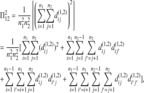 |
(A6) |
where  is the difference between sequence i of sample 1 and sequence j of sample 2. Since there is no order structure in either sample 1 or sample 2, i and i′ are just two randomly picked sequences from sample 1, and j and j′ are just two randomly picked sequences from sample 2, so that
 |
(A7) |
Under the null hypothesis,  has the same statistical property as
  or
or  so that in the remaining text of appendix a we just write it as
  regardless of where sequence i or j comes from. According to Tajima (1983),
 |
(A8) |
 |
(A9) |
 |
(A10) |
Combining (A4)–(A10), we have
 |
(A11) |
Similarly, we can get
 |
(A12) |
 |
(A13) |
 |
(A14) |
and
 |
(A15) |
 |
(A16) |
 |
(A17) |
Combining (A5), (A8)–(A10), and (A12)–(A17), we have
 |
(A18) |
 |
(A19) |
 |
(A20) |
Combining (A2), (A3), (A11), and (A18)–(A20) with (A1), we finally get (2).
APPENDIX B
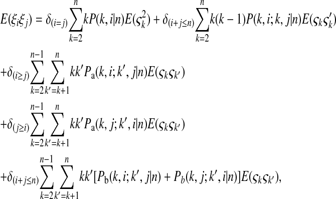
Fu (1995) showed, for a single sample,
 |
(B1) |
where  is the number of mutations whose frequency is i. δ is an index variable so that it takes the value 1 if all conditional statements in parentheses are true and takes the value 0 otherwise. Define state k as the time period in history during which the sample has exactly k ancestral sequences. Then
  is number of mutations accumulated on one of the ancestral sequences during state k, and ς′k is number of mutations accumulated on another ancestral sequence during state k,
 |
(B2) |
 |
(B3) |
 |
(B4) |
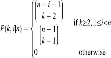 |
(B5) |
is the probability that an ancestral sequence at state k has i descendants in the sample,w
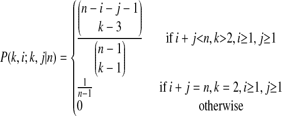 |
(B6) |
is the probability that two randomly chosen ancestral sequences at state k are of size i and j in the sample,
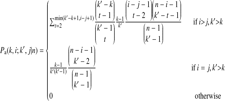 |
(B7) |
is the probability that an ancestral sequence at state k and one of its descendant sequences at state k′ (k′ > k) are of size i and j, respectively, in the sample, and
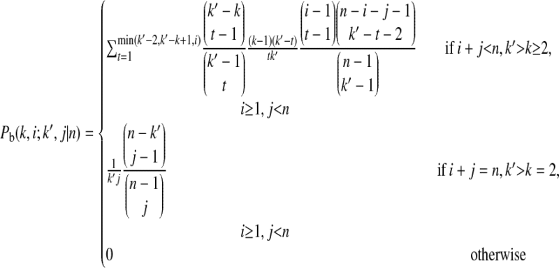 |
(B8) |
is the probability that an ancestral sequence at state k and one of its nondescendant sequences at state k′ (k′ > k) are of size i and j, respectively, in the sample.
Extending (B1) for two samples under null hypothesis, we have
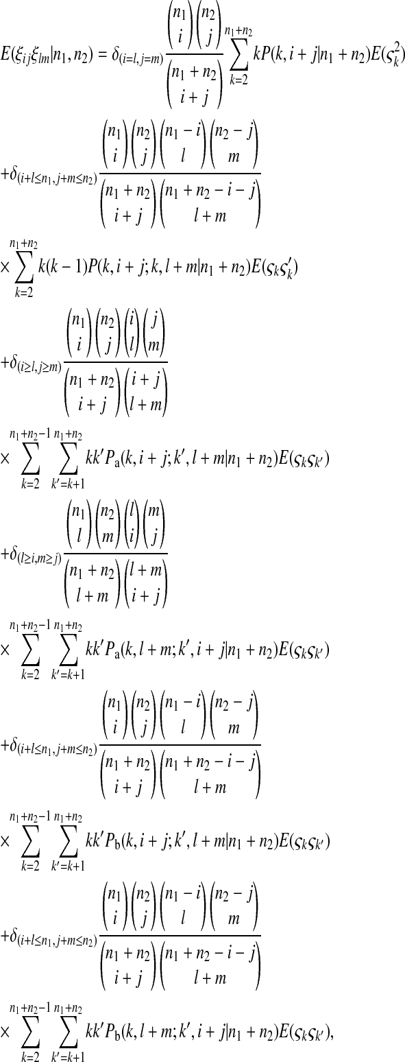 |
(B9) |
where  is the number of mutations whose frequency is i in sample 1 and j in sample 2.
 is the probability an ancestral sequence at state k has i descendants in sample 1 and j descendants in sample 2.
 is the probability that one ancestral sequence at state k has i descendants in sample 1 and j descendants in sample 2 while at the same time another ancestral sequence at state k has l descendants in sample 1 and m descendants in sample 2.
 is the probability that an ancestral sequence at state k has i descendants in sample 1 and j descendants in sample 2 while at the same time one of its descendant sequences at state k′ (k′ > k) has l descendants in sample 1 and m descendants in sample 2.
 is the probability that an ancestral sequence at state k has i descendants in sample 1 and j descendants in sample 2 while at the same time one of its nondescendant sequences at state k′ (k′ > k) has l descendants in sample 1 and m descendants in sample 2.
After some algebra, we can simplify (B9) to (13).
References
- Achaz, G., S. Palmer, M. Kearney, F. Maldarelli, J. W. Mellors et al., 2004. A robust measure of HIV-1 population turnover within chronically infected individuals. Mol. Biol. Evol. 21 1902–1912. [DOI] [PubMed] [Google Scholar]
- Drummond, A., and A. G. Rodrigo, 2000. Reconstructing genealogies of serial samples under the assumption of a molecular clock using serial-sample UPGMA. Mol. Biol. Evol. 17 1807–1815. [DOI] [PubMed] [Google Scholar]
- Drummond, A., R. Forsberg and A. G. Rodrigo, 2001. The inference of stepwise changes in substitution rates using serial sequence samples. Mol. Biol. Evol. 18 1365–1371. [DOI] [PubMed] [Google Scholar]
- Drummond, A. J., G. K. Nicholls, A. G. Rodrigo and W. Solomon, 2002. Estimating mutation parameters, population history and genealogy simultaneously from temporally spaced sequence data. Genetics 161 1307–1320. [DOI] [PMC free article] [PubMed] [Google Scholar]
- Drummond, A. J., O. G. Pybus, A. Rambaut, R. Forsberg and A. G. Rodrigo, 2003. Measurably evolving populations. Trends Ecol. Evol. 18 481–488. [Google Scholar]
- Ewens, W. J., and G. R. Grant, 2005. Statistical Methods in Bioinformatics: An Introduction. Springer, New York.
- Felsenstein, J., 1992. Estimating effective population size from samples of sequences: a bootstrap Monte Carlo integration method. Genet. Res. 60 209–220. [DOI] [PubMed] [Google Scholar]
- Fu, Y. X., 1994. A phylogenetic estimator of effective population-size or mutation-rate. Genetics 136 685–692. [DOI] [PMC free article] [PubMed] [Google Scholar]
- Fu, Y. X., 1995. Statistical properties of segregating sites. Theor. Popul. Biol. 48 172–197. [DOI] [PubMed] [Google Scholar]
- Fu, Y. X., 2001. Estimating mutation rate and generation time from longitudinal samples of DNA sequences. Mol. Biol. Evol. 18 620–626. [DOI] [PubMed] [Google Scholar]
- Fu, Y. X., and W. H. Li, 1999. Coalescing into the 21st century: an overview and prospects of coalescent theory. Theor. Popul. Biol. 56 1–10. [DOI] [PubMed] [Google Scholar]
- Griffiths, R. C., and S. Tavare, 1994. Simulating probability-distributions in the coalescent. Theor. Popul. Biol. 46 131–159. [Google Scholar]
- Hudson, R. R., 1983. Testing the constant-rate neutral allele model with protein-sequence data. Evolution 37 203–217. [DOI] [PubMed] [Google Scholar]
- Hudson, R. R., D. D. Boos and N. L. Kaplan, 1992. A statistical test for detecting geographic subdivision. Mol. Biol. Evol. 9 138–151. [DOI] [PubMed] [Google Scholar]
- Kuhner, M. K., J. Yamato and J. Felsenstein, 1995. Estimating effective population size and mutation rate from sequence data using Metropolis-Hastings sampling. Genetics 140 1421–1430. [DOI] [PMC free article] [PubMed] [Google Scholar]
- Rambaut, A., 2000. Estimating the rate of molecular evolution: incorporating non-contemporaneous sequences into maximum likelihood phylogenies. Bioinformatics 16 395–399. [DOI] [PubMed] [Google Scholar]
- Rodrigo, A. G., E. G. Shpaer, E. L. Delwart, A. K. N. Iversen, M. V. Gallo et al., 1999. Coalescent estimates of HIV-1 generation time in vivo. Proc. Natl. Acad. Sci. USA 96 2187–2191. [DOI] [PMC free article] [PubMed] [Google Scholar]
- Rodrigo, A. G., M. Goode, R. Forsberg, H. A. Ross and A. Drummond, 2003. Inferring evolutionary rates using serially sampled sequences from several populations. Mol. Biol. Evol. 20 2010–2018. [DOI] [PubMed] [Google Scholar]
- Seo, T. K., J. L. Thorne, M. Hasegawa and H. Kishino, 2002. a Estimation of effective population size of HIV-1 within a host: a pseudomaximum-likelihood approach. Genetics 160 1283–1293. [DOI] [PMC free article] [PubMed] [Google Scholar]
- Seo, T. K., J. L. Thorne, M. Hasegawa and H. Kishino, 2002. b A viral sampling design for testing the molecular clock and for estimating evolutionary rates and divergence times. Bioinformatics 18 115–123. [DOI] [PubMed] [Google Scholar]
- Tajima, F., 1983. Evolutionary relationship of DNA-sequences in finite populations. Genetics 105 437–460. [DOI] [PMC free article] [PubMed] [Google Scholar]
- Wakeley, J., and J. Hey, 1997. Estimating ancestral population parameters. Genetics 145 847–855. [DOI] [PMC free article] [PubMed] [Google Scholar]
- Watterson, G. A., 1975. Number of segregating sites in genetic models without recombination. Theor. Popul. Biol. 7 256–276. [DOI] [PubMed] [Google Scholar]


