Diploid genome reconstruction of Ciona intestinalis and comparative analysis with Ciona savignyi

Abstract

One of the main goals in genome sequencing projects is to determine a haploid consensus sequence even when clone libraries are constructed from homologous chromosomes. However, it has been noticed that haplotypes can be inferred from genome assemblies by investigating phase conservation in sequenced reads. In this study, we seek to infer haplotypes, a diploid consensus sequence, from the genome assembly of an organism, Ciona intestinalis. The Ciona intestinalis genome is an ideal resource from which haplotypes can be inferred because of the high polymorphism rate (1.2%). The haplotype estimation scheme consists of polymorphism detection and phase estimation. The core step of our method is a Gibbs sampling procedure. The mate-pair information from two-end sequenced clone inserts is exploited to provide long-range continuity. We estimate the polymorphism rate of Ciona intestinalis to be 1.2% and 1.5%, according to two different polymorphism counting schemes. The distribution of heterozygosity number is well fit by a compound Poisson distribution. The N50 length of haplotype segments is 37.9 kb in our assembly, while the N50 scaffold length of the Ciona intestinalis assembly is 190 kb. We also infer diploid gene sequences from haplotype segments. According to our reconstruction, 85.4% of predicted gene sequences are continuously covered by single haplotype segments. Our results indicate 97% accuracy in haplotype estimation, based on a simulated data set. We conduct a comparative analysis with Ciona savignyi, and discover interesting patterns of conserved DNA elements in chordates.

Genetic variation can be discovered in a genome sequencing project when homologous chromosomes are sequenced. The most abundant example of genetic variation is single-nucleotide polymorphism (SNP). SNP detection in genome sequencing projects is enabled by observing and quantifying inconsistencies in assemblies. If a significant inconsistency is observed at the same position of an assembly layout, the position can be regarded as a SNP. In the human genome, for instance, large-scale SNP discovery was facilitated by the reduced representation shotgun sequencing (Altshuler et al. 2000) and heterozygosity identification in the overlapping regions of clones (Taillon-Miller et al. 1998). In the Ciona intestinalis and Fugu rubripes genome, a SNP was called if each allele at the SNP site was observed at least twice (Aparicio et al. 2002; Dehal et al. 2002); in the Candida albicans genome, a SNP was called if the posterior probability of heterozygosity was >0.99 (Jones et al. 2004).

Once a genome is sequenced and SNP sites are detected, high-throughput SNP genotyping methods, requiring the prior knowledge of SNP-flanking sequences, are useful to obtain population genotype data (Pastinen et al. 1997; Chen et al. 1998; Wang et al. 1998). From population SNPs, in silico haplotyping methods can be used to infer haplotypes, providing more information in genetic studies. Haplotype analysis is considered to be more powerful than single-marker analysis in linkage disequilibrium studies, disease association studies, and drug response (Drysdale et al. 2000; Daly et al. 2001). In silico haplotyping methods can be categorized as those based on the parsimony principle (Clark 1990), the EM algorithm (Excoffier and Slatkin 1995; Hawley and Kidd 1995; Long et al. 1995), the Gibbs sampling methods (Stephens et al. 2001; Niu et al. 2002), and the phylogenetic structure (Bafna et al. 2003; Halperin and Eskin 2004).

Although haplotypes are often inferred from population SNPs, haplotypes can be inferred directly from genome assemblies, because phase information between adjacent polymorphisms is preserved by shotgun reads and mate-pair information. Due to the random fluctuation of sequence coverage, haplotypes are often discontinuous, resulting in a set of haplotype segments. The haplotyping problem associated with sequencing projects, referred to as the SNP haplotyping problem, was recognized and proved to be NP-hard (Lancia et al. 2001). Lancia et al. (2001) presented an algorithmic solution without simulation results. The haplotypes of Ciona savignyi were assembled by a variation of the whole-genome shotgun approach (Vinson et al. 2005). In their work, a “splitting rule” was imposed on the algorithms of the Arachne assembler to assemble split haplotypes (Batzoglou et al. 2002; Jaffe et al. 2003; Vinson et al. 2005). The split haplotypes were aligned and subsequently merged to produce a haploid consensus sequence. In our previous work (Li et al. 2004), we proposed a statistical method to infer haplotypes from genome assemblies by extending the earlier method to estimate the quality of a haploid consensus sequence (Churchill and Waterman 1992). The basic principle of our previous method was that the most likely haplotypes were inferred from every two adjacent SNPs and connected according to their phase consistencies. As we assumed that polymorphic sites were known, the pair-based approach was an efficient solution in the simulation studies.

In real genome sequencing projects, however, the SNP detection problem is inherently related to the SNP haplotyping problem. Under our probabilistic model, the solution to the two problems can be improved by controlling two inter-related tradeoffs: (1) a tradeoff between sensitivity and specificity in the SNP detection problem, and (2) a tradeoff between sensitivity and complexity in the SNP haplotyping problem. Obviously, we lose specificity as we gain sensitivity in the SNP detection problem and vice versa. In the SNP haplotying problem, our haplotype estimation is more robust to sequencing errors if haplotypes are inferred from more than a pair of potential SNP sites. However, the number of possible haplotypes grows exponentially with the number of potential SNP sites [O(5²ⁿ)]. As we gain sensitivity in the SNP detection problem, haplotypes are inferred from potential SNP sites that contain many non-SNP sites. Consequently, the complexity in the SNP haplotyping problem increases. The pair-based approach shows limited performance to handle the two inter-related tradeoffs.

In this study, we use a model selection method to detect potential SNPs from genome assemblies. To infer haplotypes from detected potential SNPs, we use a Gibbs sampling method, which is a Markov Chain Monte Carlo (MCMC) algorithm (Liu 2002). By integrating the Gibbs sampling method with the model selection method, we control the two tradeoffs, thereby inferring haplotypes from multiple potential SNPs. Our method accommodates two-end sequenced reads of clones such as plasmids, cosmids, or bacterial artificial chromosomes (BACs). Mate-pair information is exploited to extend haplotypes beyond an assembled contig. We selected the Ciona intestinalis genome to infer haplotypes from a real genome assembly because its reported polymorphism rate (1.2%) was high and the libraries were mostly prepared from a single individual (Dehal et al. 2002). The accuracy of our method is studied using a simulated data set, where true haplotypes are assumed to be known. Throughout this study, we limit genetic variation between two homologous chromosomes to SNPs (including single indels), multibase substitutions, and multibase indels. Hereafter, the term polymorphism includes SNPs, multibase substitutions, and multibase indels.

Results and Discussion

The Ciona intestinalis genome

The study of the ascidian, Ciona intestinalis, gives insights into the divergence of the chordates from the deuterostomes and the vertebrates from the chordates (Dehal et al. 2002). A whole-genome shotgun approach was taken to sequence the genome of Ciona intestinalis by the Joint Genome Institute (JGI). DNA was purified mainly from the sperm of an individual in Half Moon Bay, California, USA; the BAC and cosmid libraries were prepared in part from a Japanese individual and a different California individual, respectively (Dehal et al. 2002). We constructed an assembly by aligning shotgun reads to the reference genome sequence of Ciona intestinalis (see Methods).

Diploid consensus sequence

As sequence coverage decreases, haplotype estimation often halts prematurely, and thus yields a set of disjoint haplotype segments. A segmental example of the diploid consensus sequence is shown in Figure 1. A total of 1,595,673 polymorphisms were identified at the base level in all the regions spanned by at least one read, and 1,314,870 polymorphisms were identified if a multibase polymorphism is counted once. Accordingly, the polymorphism rates were 1.5% (at the base level) and 1.2%, respectively. A total of 64,358 multibase substitutions and 73,379 multibase indels were identified, even though heterozygosity is mostly accounted for by single substitutions. We identified 1,107,913 single substitutions with 69,221 single indels. At the base level, 59% of substitutions are transitions and 41% are transversions; 46.1% of polymorphisms are located in introns, 8.5% in exons, 1.9% in untranslated regions (UTRs), and 43.5% in intergenic (unannotated) regions.

Figure 1.

Example of the diploid genome sequence from the scaffold_1. The diploid consensus sequence is shown at the top. Polymorphic sites and sequencing errors are represented as uppercase.

As reported in the Ciona savignyi genome (Vinson et al. 2005), the distribution of polymorphisms is highly variable across the Ciona intestinalis genome. To illustrate this variability, we slid a 1000-bp window along the genome and counted the number of polymorphisms in each window. Figure 2 (from the scaffold 24) indicates that the distribution of polymorphisms is not uniform across the genome; as many as 59 polymorphisms were observed in a window, although no polymorphism was observed in some of the other windows. Therefore, a Poisson model is inappropriate to explain the overdispersion. We counted the number of polymorphisms in nonoverlapping 200-bp windows across the genome, and calculated the mean and variance (μ = 2.48, σ² = 8.1). The coalescent theory predicts that the number of substitutions in windows fits a compound Poisson distribution (with exponential rate) (Huelsenbeck and Nielsen 1999; Nordborg 2001), as shown in Figure 3.

Figure 2.

Distribution of polymorphisms on the scaffold_24. The positions of windows along the genome are shown on the X-axis and the number of polymorphisms in window is shown on the Y-axis. Multibase substitutions and multibase indels were counted at the base level.

Figure 3.

Probability distribution of polymorphism rates in 200-bp windows. Black bar indicates the probability that the given number of polymorphisms is observed in 200-bp windows. Dark gray bars indicate the probability predicted by the coalescent theory, which well fits our observation in the Ciona intestinalis genome. However, a geometric distribution, indicated by light gray bars, does not fit our observations.

Diploid gene sequences

In total, 15,852 genes were predicted from the Ciona intestinalis project (Dehal et al. 2002). We could align 15,410 (97.2%) gene sequences to the diploid consensus sequence by using BLAT (default parameters) (Kent 2002). A total of 442 gene sequences were not aligned, because 5% of the entire set of scaffolds was not covered by our map alignments. Of the 15,410 gene sequences, 13,166 (85.4%) gene sequences were aligned within haplotype segments, not being interrupted by any discontinuity. Therefore, diploid gene sequences could be continuously inferred from those 13,166 predicted gene sequences. Each of 1019 gene sequences spanned two adjacent haplotype segments, being interrupted by a single disconnection. Discontinuous diploid gene sequences could be inferred from the 1019 predicted gene sequences. We summarize the full results in Figure 4.

Figure 4.

Discontinuity of diploid gene sequences. A total of 13,166 (85.4%) diploid gene sequences are continuously estimated, lying completely within haplotype segments. Each of 1019 diploid gene sequences consists of two segments, disconnected once along the sequence. Therefore, each of 14,185 (13,166 + 1019; 92%) diploid gene sequences is disconnected, at most, once. Each of 636 diploid gene sequences is disconnected twice. Therefore, each of 14,821 (13,166 + 1019 + 636; 96.2%) diploid gene sequences consists of, at most, three segments.

Although sequences are discontinuous in 14.6% of the predicted genes, discontinuous diploid gene sequences are possibly useful if those segments take the majority of the predicted genes. In 91.7% of the predicted genes, the longest segment covered more than 70% of the entire gene sequence (Table 1). The continuity of the diploid gene sequences is mainly attributed to the abundance of polymorphisms in introns and shortness of exons in the Ciona intestinalis genome (Dehal et al. 2002).

Table 1.

Continuity of diploid gene sequences

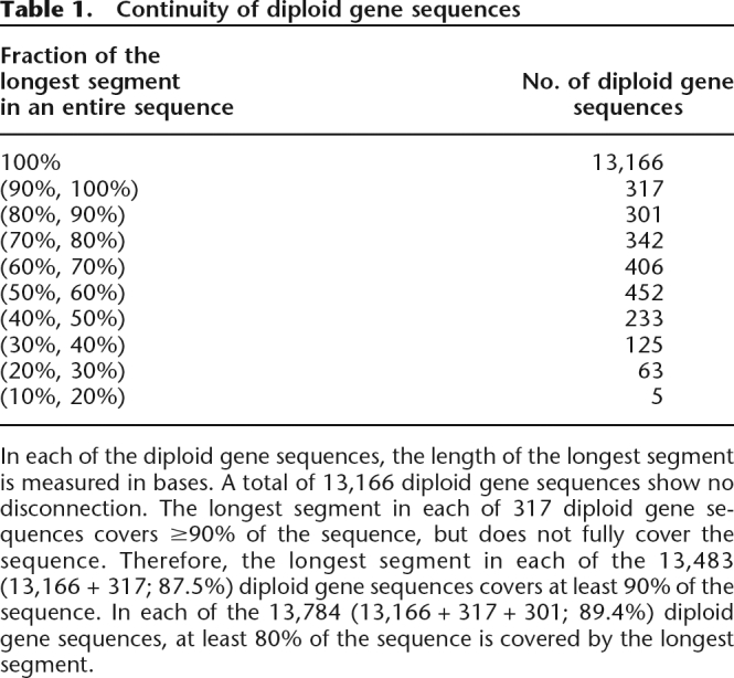
In each of the diploid gene sequences, the length of the longest segment is measured in bases. A total of 13,166 diploid gene sequences show no disconnection. The longest segment in each of 317 diploid gene sequences covers ≥90% of the sequence, but does not fully cover the sequence. Therefore, the longest segment in each of the 13,483 (13,166 + 317; 87.5%) diploid gene sequences covers at least 90% of the sequence. In each of the 13,784 (13,166 + 317 + 301; 89.4%) diploid gene sequences, at least 80% of the sequence is covered by the longest segment.

Simulated sequences

The accuracy of our method was studied through simulation. From the published draft genome sequence of Ciona intestinalis, the artificial polymorphic sites were generated uniformly across the genome according to the rate reported by our method. Single indels, multibase substitutions, and multibase indels were also generated, reflecting their actual proportions and lengths in the real data. After the assembly layout was constructed by the aforementioned pairwise alignments, the origin of each read was randomly generated with probability 1/2 (one of two chromosomes). The sequencing error rate was based on the real quality score of each base-call and our error model (see Equation 1 in Methods). In this simulation, the accuracy of our estimation could be evaluated because the true haplotypes were known.

Considering the polymorphism rate from the real data set, we generated 1,940,074 true polymorphisms. Among these positions, 286,862 polymorphisms were not observable due to failure to sample one or both genomes. In total, we identified 1,598,604 polymorphisms. Given the known true haplotypes, we were able to compare estimated haplotype segments with the corresponding regions of the true haplotypes. If bases in estimated haplotype segments exactly matched the corresponding bases in the true haplotypes, these bases in estimated haplotype segments were counted as true positives. Otherwise, the bases in estimated haplotype segments were counted as false positives. According to this calculation, the true positive rate was 97.01%. Among the false positives, some of the bases showed inverted phases, while polymorphisms were correctly detected. Those inverted bases were 2.23% of our haplotype estimation. A total of 0.75% was estimated to be heterozygous, which is originally homozygous, and 0.01% of detected polymorphisms were incorrect, although one allele of the estimated polymorphism was matched with one allele of the true polymorphism at each position. Most errors were caused by sequencing errors in low-coverage regions (sequence coverage <4×). A low false negative rate (4.03%) was achieved, which indicates that most of the polymorphisms are detectable by our method.

The Ciona savignyi genome

A related species in the Ciona genus, Ciona savignyi, was assembled by Vinson et al. (2005). Notably, the Ciona savignyi genome is much more polymorphic (polymorphism rate: 4.6%) than the Ciona intestinalis genome (polymorphism rate: 1.2%). The two Ciona species have been previously known to be very distant (Johnson et al. 2004). Our whole-genome comparison (see Methods) also shows that the two Ciona genomes are highly divergent from each other at the base level. Using a definition of conservation (length ≥100 bp, identity ≥70%) by other studies (Dermitzakis et al. 2002; Nobrega et al. 2004), 1835 conserved elements were identified (lengths: 100 bp ∼ 4987 bp, average: 408.6 bp), which account for 0.7% of the Ciona intestinalis genome.

As explained above, polymorphisms are enriched in the Ciona intestinalis genome (1.5% at the base level). Polymorphism rates are higher in noncoding regions, introns (1.85%), and intergenic regions (1.47%), than in coding regions (0.8%). Aligning the conserved elements to the diploid consensus sequence, we observed that the polymorphism rate in the conserved elements (0.53%) is lower than the overall rate (1.5%). Restricted to the conserved elements, we further examined the polymorphism rate within each region annotated as a different type by annotating the conserved elements at the base level. In the conserved elements, polymorphism rates are slightly lower in noncoding regions, introns (0.51%), and intergenic regions (0.49%), than in coding regions (0.57%), although the criteria for the conserved elements are defined regardless of annotation type. This trend becomes more evident as we use more stringent thresholds to define conserved elements (length ≥100 bp, identity ≥80%), identifying 899 conserved elements. The polymorphism rate is further lowered in noncoding regions, introns (0.34%) in intergenic regions (0.34%), while the polymorphism rate in coding regions (0.57%) remains constant.

Of the 1835 conserved elements (length ≥100 bp, identity ≥70%), 932 (51%) conserved elements overlapped exons, and no conserved element completely fell within introns. The percentage of conserved elements overlapping exons is close to that of “highly conserved elements” (HCE) overlapping genes (42% overlapping exons and 19% completely falling within introns) in vertebrates, although the definition of HCEs is different from our definition of conserved elements (Siepel et al. 2005). In insects, worms, and yeast, HCEs are much more likely to overlap coding exons (93% in insects, 98% in worms, and 99% in yeast) (Siepel et al. 2005). From the observations in vertebrates, insects, worms, and yeast, Siepel et al. (2005) predicted a general tendency that the percentage of HCEs overlapping genes is strongly associated with genome size and gene density. Although we attempted to use more stringent criteria to define conserved elements (length ≥100 bp, identity ≥80%; length ≥100 bp, identity ≥90%; length ≥200 bp, identity ≥70%) than the previous criterion (length ≥100 bp, identity ≥70%), the percentage of conserved elements overlapping exons in the Ciona genomes (Fig. 5, left) was lower than that in insects, worms, and yeast. Our results indicate that the less association of conserved elements with genes and more association with intergenic regions are also observed in a simple invertebrate chordate with a compact genome (estimated to be a total of 159 Mb) (Dehal et al. 2002).

Figure 5.

(Left) Fractions of conserved elements overlapping exons and intergenic regions. (Right) Annotation of conserved elements at the base level. In this figure, the calculation of fractions is based on the predicted gene sequences in the reference genome, Ciona intestinalis. From the top row to the bottom row, the thresholds to define conserved elements and the number of identified conserved elements are as follows: (first row) length ≥100 bp, identity ≥70%, 1835 elements; (second row) length ≥100 bp, identity ≥80%, 899 elements; (third row) length ≥100 bp, identity ≥90%, 91 elements; (fourth row) length ≥200 bp, identity ≥70%, 1112 elements.

In the Ciona intestinalis genome, the conserved elements associated with exons tend to be longer and less identical than the conserved elements in intergenic regions and introns. As shown in Figure 5, left, the percentage associated with intergenic regions increases as we use more stringent thresholds (identity ≥80% or identity ≥90%) for the identity of conserved elements. On the other hand, the percentage associated with exons increases as we use a more stringent threshold (length ≥200 bp) for the length of conserved elements (Fig. 5, left). In Figure 5, right, we annotated conserved elements at the base. As shown in Figure 5, the fraction of bases in noncoding regions increases as we increase the threshold level for the identity of conserved elements (≥80% or ≥90%). The fraction of bases in coding regions increases as we apply the threshold level (≥200 bp) for the length of conserved elements.

Overall, the results from our comparative analysis are not fully consistent with the predictions from Siepel et al. (2005) when the assembled genome sizes of the two Ciona species are considered (116.7 Mb and 157 Mb) (Dehal et al. 2002; Vinson et al. 2005). One possible explanation is that in the Ciona intestinalis genome, relatively short noncoding regions, possibly regulatory elements, are under strong constraints, playing critical roles in gene regulation. It has been consistently reported that a significant number of conserved regions are associated with nonexonic regions in vertebrates, including humans (Dermitzakis et al. 2002; Bejerano et al. 2004; Siepel et al. 2005). In particular, of the 481 extremely conserved elements in the human, rat, and mouse genomes (identity = 100%, length ≥200 bp), called “Ultraconserved elements,” 256 ultraconserved elements are associated with noncoding regions. Our comparative analysis of the two Ciona species shows a strong association of conserved elements with noncoding regions, suggesting that conservation in noncoding regions possibly characterizes a pattern of evolution in chordates, including vertebrates, not necessarily correlated with genome size and gene density.

Diploid assembly of polymorphic genomes

It has been known that the enrichment of polymorphisms in a genome significantly undermines assembly continuity (Aparicio et al. 2002; Dehal et al. 2002; Jones et al. 2004; Vinson et al. 2005). In the presence of enriched polymorphisms, it is often difficult to determine a threshold level between true and false overlaps of sequenced reads during an assembly process. This problem becomes more severe as polymorphism rates increase, further indicated by genomic repeats. Although other factors, such as repeat content, library quality, sequence coverage, and assembly strategy, also influence assembly continuity (Vinson et al. 2005), the problem is highlighted when we compare the N50 scaffold length of the human genome with the N50 scaffold length of the Ciona intestinalis genome (2.7 Mb vs. 190 kb) (Dehal et al. 2002; Istrail et al. 2004).

Once polymorphic genomes are assembled, the genomes are prominent resources from which to reconstruct haplotypes, because a sequenced read covers several polymorphisms. In general, however, current genome sequencing projects have published haploid genome sequences without reconstructing haplotypes. The only exception is the diploid assembly of Ciona savignyi (Vinson et al. 2005). In the Ciona savignyi sequencing project, haplotypes were assembled while a haploid consensus sequence was published. The rationale of this approach is that in highly polymorphic organisms haplotypes can be separated into distinct scaffolds in the overlap detection step of an assembly process. In this approach, haplotypes are first assembled into separate haploid scaffolds. These haploid scaffolds are then merged into diploid scaffolds. The N50 scaffold length of the Ciona savignyi genome was significantly increased, compared with the N50 scaffold length of the Ciona intestinalis genome (989 kb vs. 190 kb) (Dehal et al. 2002; Vinson et al. 2005). It should be noted that the diploid assembly of Ciona savignyi is remarkable in terms of assembly continuity. It appears that the process to differentiate haplotypes is facilitated when two conditions are satisfied. First, it appears that high sequence coverage is very helpful to assemble each haploid scaffold prior to mergence. The sequence coverage in the Ciona savignyi sequencing project was much higher than the sequence coverage in the Ciona intestinalis project (13× vs. 8×) (Dehal et al. 2002; Vinson et al. 2005). Second, the approach is more suitable to organisms with very high levels of polymorphism. In sequenced reads, there should be sufficient polymorphisms to separate a haplotype from the opposite haplotype. Because the estimated polymorphism rate of Ciona savignyi was 4.6% (Vinson et al. 2005), haplotypes were very likely to be assembled into separate haploid scaffolds.

Several strategies have been developed to assemble polymorphic genomes according to the polymorphism rates of the target genomes (Aparicio et al. 2002; Dehal et al. 2002; Jones et al. 2004; Vinson et al. 2005). We see that it is still a challenging problem to assemble polymorphic genomes under 7× or 8× sequence coverage. It also remains a challenge to assemble polymorphic genomes with a single strategy, regardless of their polymorphism rates (Vinson et al. 2005). In this study, we focus on reconstructing haplotypes (equivalently, diploid consensus sequence) from genome assemblies, avoiding the issue of assembling polymorphic genomes. For this reason, our method is applicable regardless of assembly strategies.

Obviously, however, our method has some limitations. First, the lengths of sequenced reads and the polymorphism rates are critical to the performance of our method whether mate-pair information is used or not. We have tested our method, fixing the average length of sequenced reads as 550 bp. As shown in Table 2, our simulation results indicate that the performance of our method is very limited as the polymorphism rate falls below 0.2%. Unless the application of our method is restricted to polymorphic regions (for example, genes where polymorphisms are enriched) or longer reads are sequenced, our method is not very useful to infer haplotypes from mammalian genomes such as the human and chimpanzee genome (Lander et al. 2001; Venter et al. 2001; Mikkelsen et al. 2005). Second, although our method does not handle the problem of assembling polymorphic genomes, the quality of estimated haplotypes depends on the quality of diploid assembly. Haplotype estimation is degraded if a haplotype and the opposite haplotype are assembled into separate scaffolds, or genomic repeats are misplaced in scaffolds. Third, our model assumes the existence of two haplotypes from a single individual. Haplotype estimation is also degraded to some extent if this assumption is violated in genome assemblies.

Table 2.

N50 length of haplotype segments by varying sequence coverage and polymorphism rate

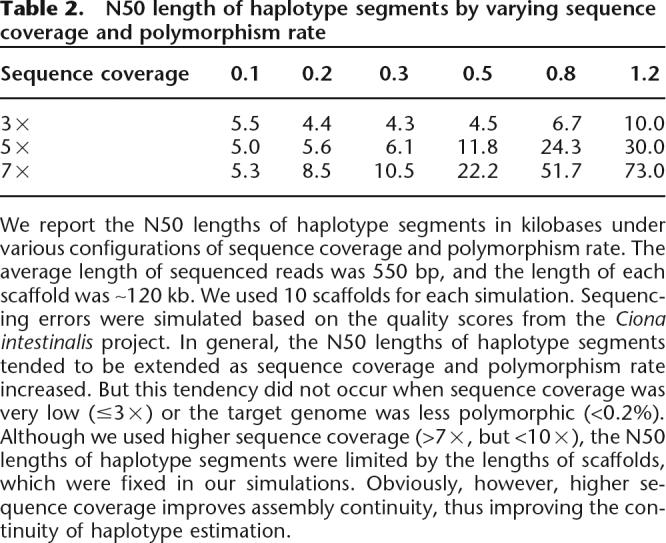
We report the N50 lengths of haplotype segments in kilobases under various configurations of sequence coverage and polymorphism rate. The average length of sequenced reads was 550 bp, and the length of each scaffold was ∼120 kb. We used 10 scaffolds for each simulation. Sequencing errors were simulated based on the quality scores from the Ciona intestinalis project. In general, the N50 lengths of haplotype segments tended to be extended as sequence coverage and polymorphism rate increased. But this tendency did not occur when sequence coverage was very low (≤3×) or the target genome was less polymorphic (<0.2%). Although we used higher sequence coverage (>7×, but <10×), the N50 lengths of haplotype segments were limited by the lengths of scaffolds, which were fixed in our simulations. Obviously, however, higher sequence coverage improves assembly continuity, thus improving the continuity of haplotype estimation.

Sequencing errors mildly affect haplotype estimation, unless sequencing errors occur in the regions less covered by reads (sequence coverage <4×). Most of phase-inversion errors occur in those low-coverage regions because phases are not sufficiently supported by data. Therefore, high coverage is beneficial to haplotype estimation, decreasing the noise effect from sequencing errors and increasing the chance that over regions, reads are sampled from two haplotypes. When we assume that the lengths of sequenced reads are constant across a genome sequencing project, the continuity of estimated haplotype segments depends on polymorphism rate and sequence coverage as indicated in Table 2. We suggest at least 7× sequence coverage, although 5× sequence coverage performs remarkably well for the elevated level of continuity in haploid assembly (Istrail et al. 2004). Table 2 indicates that 0.1% polymorphism rate is too low to take the advantage of increased sequence coverage. Because our method favors local information (see Methods), small clone inserts (1.8 kb ∼ 3 kb) are more useful than longer clone inserts (∼120 kb) to extend haplotypes. But the usage of the long clone inserts is justified to assemble elongated scaffolds during the assembly process.

N50 length of haplotype segments

In the Ciona savignyi assembly, Vinson et al. (2005) calculated the N50 length of haplotype segments without extending haplotype segments beyond intra-scaffold gaps. Their haplotype segments were defined to be consecutive sequences, not being interrupted by intra-scaffold gaps. According to this definition, the N50 length of haplotype segments was 21.4 kb.

In our method, if mate-pair information significantly supports extensions, haplotype segments are extended beyond intra-scaffold gaps, intrinsically containing intra-scaffold gaps. Here, haplotype segments are defined to encompass intra-scaffold gaps if flanking contigs are extended by mate-pair information. According to our definition, the N50 length of haplotype segments was 37.9 kb (average length: 9.3 kb) in the Ciona intestinalis assembly. In Supplemental Figure S1, the distribution of the lengths of reconstructed haplotype segments is shown. Compared with the N50 length of haplotype segments in the real data set, the longer N50 length of haplotype segments (68.6 kb, average length: 14 kb) was attained in the simulated data set because the complexity, arising in the Ciona intestinalis sequencing project, was eliminated; the main differences are that: (1) no misassembly was assumed, (2) sequence reads were assumed to originate from a single individual, and (3) recombinants were not simulated.

It was reported that highly polymorphic organisms are subject to misassembly (Jones et al. 2004; Vinson et al. 2005). For simplicity, we assumed that the assembly was correct in our simulation. Because DNA was extracted from sperm in the Ciona intestinalis sequencing project, there were recombinations that mildly affect phase determination. Based on a statistical model, our method is not sensitive to the rare recombination events. Therefore, we ignore recombinants in our simulation. In the Ciona intestinalis sequencing project, ∼10% of sequence reads originated from different individuals. Obviously, adding external sequence reads made the N50 length of haplotype segments shorter.

Confidence of diploid consensus sequence

To assess the accuracy of diploid consensus sequences and to identify low-quality regions, it is necessary to provide a statistical confidence measure. Although this assessment is straightforward in a haploid consensus sequence (Churchill and Waterman 1992), the consideration of the phase between polymorphisms is required to assess a diploid consensus sequence. For this reason, we developed a confidence measure to assess estimated diploid consensus sequences, where PHRED quality scores are used as an input (Kim et al. 2007).

Multiple-haplotype reconstruction

In the genome project where libraries are prepared from many individuals (greater than two), there can be multiple haplotypes instead of only two haplotypes. An extreme form is the environmental genome shotgun assembly aiming at simultaneously sequencing representatives from a mixture of numerous organisms under an environment (Venter et al. 2004). Although our method currently reconstructs two haplotypes, our model selection scheme and the Gibbs sampler can be extended to reconstruct multiple haplotypes. In each region, the number of haplotypes in the Bayesian model selection is given as a parameter and the maximized model is selected. Then, the subsequent local haplotyping and haplotype extension steps (see Methods) are adapted to the selected number of haplotypes in the model.

Methods

Assembly of Ciona intestinalis

The draft genome of Ciona intestinalis, shotgun reads, and quality files were downloaded from the website of the JGI (http://genome.jgi-psf.org/ciona4). The clone inserts of variable sizes (1.8 kb ∼ 120 kb) were generated and two-end sequenced (Dehal et al. 2002). The low-quality regions of the shotgun reads were trimmed by using LUCY (Chou and Holmes 2001). The quality-trimmed shotgun reads were then aligned to the published Ciona intestinalis draft genome by using BLASTN (Altschul et al. 1997). In each pairwise alignment, we used 1 × 10⁻⁷⁸ for the E-value cutoff and default values for the other parameters. The distance between two-end sequenced reads was also considered to resolve the repeat problem. It was reported that in JGI’s protocol, ∼99% of paired reads were located within mean ± four standard deviations of their insert sizes (Aparicio et al. 2002; Dehal et al. 2002). Paired reads were included in our assembly only if they were located within this distance. The reads, which were missing a paired end, were also included in the assembly if the reads were uniquely mapped to the reference genome. After intra-scaffold gaps were removed, the alignments spanned 95% of the draft genome; total size including the intra-scaffold gaps is 116.7 Mb (Dehal et al. 2002). The sequence coverage was ∼8×, which is consistent with the reported sequence coverage (Dehal et al. 2002). To minimize the possibility that sequencing errors are called polymorphisms over less-covered regions (≤6×), we excluded the bases not meeting a “neighborhood quality standard” (NQS) condition over those regions; a base satisfies the NQS condition if the base has PHRED score ≥20, and the flanking five bases on each side have PHRED scores ≥15 (Altshuler et al. 2000). We also excluded low-quality bases (≤4×) over all regions.

Whole-genome alignment

Downloading the Ciona savignyi genome sequence from the Ensembl website (http://www.ensembl.org), we used a whole-genome aligner, MUMmer, to identify conserved elements (Kurtz et al. 2004). Considering the divergence of the two organisms, we increased the sensitivity of MUMmer by adjusting the parameters (-l: 4, -g: 3000, -c: 100, and -b: 200). If a region in one genome was aligned to multiple regions in the other genome, the most significant alignment was chosen by using the two parameters, -r and -q. Subsequently, we eliminated nonorthologous alignments originated from genomic repeats such as tandem and interspersed repeats by using RepeatMasker (http://www.repeatmasker.org/).

Haplotype reconstruction

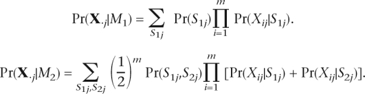
The result of sequence assembly is an assembly layout, which can be thought to be a matrix. Each row indexed by i = 1, 2, . . . , m corresponds to a sequence of bases from a fragment aligned to a genome sequence. Each column indexed by j = 1, 2, . . . , n corresponds to a particular genomic position that runs from the left to the right in the assembly layout. In the matrix, base-calls are denoted by X = {X_ij = x_ij; i = 1, 2, . . . , m, j = 1, 2, . . . , n}, and their underlying true bases by Y = {Y_ij; = y_ij; i = 1, 2, . . . , m, j = 1, 2, . . . , n}, where x_ij and y_ij take values from the alphabet sets B = {A, C, G, T, − , N, ϕ} and A = {A, C, G, T, −}, respectively; N and ϕ represent an ambiguous base-call and a null base beyond called bases in each read, respectively. Base-calls at column j are denoted by X_⋅j = {X_ij; i = 1, 2, . . . , m}. Similarly, true haplotypes are denoted by S = {S_kj = s_kj; s_kj ∈ A, k = 1, 2, j = 1, 2, . . . , n}, and the origins of fragments (clone inserts) by F = {F_i = f_i; f_i ∈ {1, 2}, i = 1, 2, . . . , m}; f_i is 1 if the fragment originates from the first chromosome, and f_i is 2 if the fragment originates from the second chromosome. For the simplicity of notation, reads are assumed to be oriented in the same direction in all cases; the general case is easily handled but complicates the formula. Fragments are two-end sequenced, and uncalled regions between paired reads are represented by ϕ in our model. It is assumed that the composition probabilities at each genomic position are independent of other positions, and these composition probabilities are constant across haplotypes. The composition probabilities are denoted by

Instead of constant sequencing error probabilities (Churchill and Waterman 1992; Li et al. 2004), position-specific PHRED quality scores are incorporated into our model (Ewing and Green 1998). Therefore, the sequencing error probabilities are denoted by

where q_ij is the PHRED quality score at row i and column j in the assembly matrix. Our haplotype reconstruction strategy consists of four steps: (1) potential polymorphism detection, (2) local haplotyping, (3) haplotype extension, and (4) haplotype bridging. The overview of the strategy is illustrated in Figure 6.

Figure 6.

Overview of our haplotype reconstruction strategy. (A) In this step, Bayesian model selection is used to detect potential polymorphic sites along a genome. Two different alleles at each polymorphic site are represented by a triangle and a rectangle. In this figure, detected polymorphic sites run from the left-hand side to the right-hand side according to their genomic positions in an assembly. (B) We determine phases among detected polymorphisms by using a Gibbs sampling method. We focus on estimating reliable haplotypes from a small number of polymorphisms by repeating the following two steps: (1) update S based on F, (2) update F based on S. (C) If adjacent short haplotypes overlap and show a consistency, those haplotypes are combined. (D) Adjacent haplotypes are connected if the fragments spanning those adjacent haplotypes significantly support the connection.

Potential polymorphism detection

Because it is computationally inefficient to infer haplotypes from all the genomic positions, a Bayesian model selection scheme is adopted to identify potential polymorphisms and reduce the number of genomic positions considered. We denote one haplotype-based model and two haplotype-based model by M₁ and M₂, respectively. For given thresholds α₁ and α₂, the j − th genomic position is screened as a potential polymorphism by computing and checking

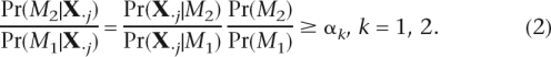Note that Pr(M₂)/Pr(M₁) is a constant factor. To control false positive and false negative rates, we specify two different thresholds, α₁, α₂ (α₂ ≫ α₁). The accuracy of polymorphism detection can be achieved by increasing α₂. However, it inevitably increases false negative rates (undetected true polymorphisms). We increase α₂ for high accuracy while maintaining α₁ sufficiently low in order not to miss true polymorphisms. The genomic positions where Equation 2 holds for k = 2 are termed strongly potential polymorphisms. Similarly, the genomic positions where Equation 2 holds for k = 1 are termed weakly potential polymorphisms. According to these criteria, all strongly potential polymorphisms are also weakly potential polymorphisms. All the genomic positions other than potential polymorphisms are regarded to be homozygous and excluded from estimation. The likelihood calculations in Equation 2 are based on the previous works (Churchill and Waterman 1992; Li et al. 2004).

After the assembly layout was constructed by aligning shotgun reads to the Ciona intestinalis draft genome sequence, the artificial polymorphic sites (rate: 1.2%) were generated along the genome sequence. Sequencing errors were simulated according to Equation 1 and the real quality scores from the Ciona intestinalis assembly. AfterPr(M₂)/Pr(M₁) was removed, α₂ and α₁ were trained and selected to be 100 (true positive rate >0.99) and 1 (false negative rate <0.03), respectively.

Local haplotyping

In this step, we compose blocks, each of which is comprised of four strongly potential polymorphisms with intervening weakly potential polymorphisms, such that an overlap (two strongly potential polymorphisms) exists between adjacent blocks (Fig. 7A,B). In the haplotype extension step, this block composition of four strongly potential polymorphisms facilitates the identification of uncertain phases among strongly potential polymorphisms. After blocks are composed, the Gibbs sampler is applied to determine the phases of each block. In our MCMC approach, a time variable t is introduced. Therefore, is S_ij at time t, and is F_i at time t. Let S_[−(i,j)] = {S_i′j′;(i′j′) ≠ (i,j)} and F_[−i] = {F_i′;i′ ≠ i}. The most likely haplotypes are sampled by repeating the following two steps.

Figure 7.

Block composition and local haplotyping. In this figure, for simplicity, only strongly potential polymorphisms are indexed by the top row, although there possibly exists weakly potential polymorphisms between adjacent strongly potential polymorphisms. Here, we index seven strongly potential polymorphisms from the (i − 1)-th position to the (i + 5)-th position. (A) Potential polymorphic sites are determined after the potential polymorphism detection step. Dotted lines between strongly potential polymorphisms indicate that their phases are not determined yet. (B) An example of block composition is shown. We compose two adjacent blocks, block_j in (1) and block_j+1 in (2). The adjacent blocks share two strongly potential polymorphisms at the (i + 2)-th and (i + 3)-th positions. (C) After the Gibbs sampler is applied to each block, the phases are determined. Each solid line indicates a direction of connection. In (1), for instance, local haplotypes_j, TCCT and CTAA, are obtained.

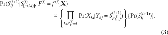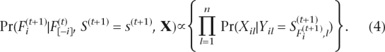We calculate the above conditional probabilities by normalizing Equations 3 and 4. To evaluate the confidence of our estimation, we define a confidence score to be Pr (the most likely haplotypes for a block observation) (Li et al. 2004; Kim et al. 2007). If the confidence score is greater than or equal to a threshold (0.9), we say that the phases for the block are determined (Fig. 7C) and term the phase-determined blocks as local haplotypes. In the following haplotype extension step, we combine at least two local haplotypes and term the results as extended haplotypes (Fig. 8A).

Figure 8.

Haplotype extension. Haplotype extension proceeds from the lower index to the higher index. (A) Haplotypes can extend over more than four strongly potential polymorphisms as the result of the previous haplotype extension. We assume that the extended haplotypes, · · · CCTAA and · · · ATCCT, are given up to the (i + 3)-th position. (B) After the local haplotypes, AACA and CTGT, are obtained in (1), the extended haplotypes in A can be combined with the local haplotypes and extended to · · · CCTAACA and · · · ATCCTGT by the consistency of shared strongly potential polymorphisms (the dashed box) at the (i + 2)-th and (i + 3)-th positions. The combined haplotypes are shown in (2). (C) In (1), an inconsistency is observed at the (i + 2)-th position. After the local haplotypes are extended to the (i + 1)-th position, the inconsistency is resolved in (2). The combined haplotypes are shown in (3). (D) Although the local haplotypes are extended in (2), the inconsistency at the (i + 2)-th position is still observed. The number of matches for two phases is calculated from the (i + 1)-th to the (i + 3)-th position (in the dotted box): in this example, 5 for one direction of connection and 0 for the other direction of connection. The resolved extension is shown in (3).

Haplotype extension

Because adjacent local haplotypes share two strongly potential polymorphisms by our block composition method, the phases of the adjacent extended haplotypes can be further extended by combining them (Fig. 8A,B). If extended haplotypes and local haplotypes are not consistent in shared strongly potential polymorphisms (Fig. 8C1), the block for local haplotypes is extended to the previous strongly potential polymorphisms, and the Gibbs sampler is applied to this extended block (Fig. 8C2). If the extended local haplotypes are consistent with the extended haplotypes, the ambiguous phase is resolved (Fig. 8C3). Otherwise, some mismatches are allowed in shared strongly potential polymorphisms; for two different directions of connection, the number of matches is calculated, and the majority direction is selected (Fig. 8D). If the confidence score of inferred haplotypes is less than a threshold, we subdivide the haplotypes, identify the uncertain connection (the confidence score < a threshold), and break the connection; we can easily identify the uncertain connection because there are only two possible locations of the weak connection when a block is comprised of four strongly potential polymorphisms (Supplemental Fig. S2).

Haplotype bridging

If the confidence score for a block is below a threshold, extension does not continue further. However, it is obvious that each fragment often covers several polymorphic sites when the polymorphism rate is high. In this haplotype bridging step, adjacent extended haplotypes are further connected by checking whether there exist fragments linking them. After extended haplotypes are constructed from the previous haplotype extension step, there exist two ways to connect adjacent extended haplotypes. Two possible configurations are denoted by C₁ and C₂, which are illustrated in Supplemental Figure S3, A and B, respectively. As illustrated in Supplemental Figure S3, the extended haplotypes on the left-hand side are denoted by and . Similarly, the extended haplotypes on the right-hand side are denoted by and . Some fragment, denoted by Z_i, spans adjacent extended haplotypes. A set of such fragments are denoted by Z = {Z_i; i ∈ I}. When a fragment Z_i spans adjacent extended haplotypes, the indexes of the polymorphic sites in and are denoted by J_i,L. Similarly, the indexes of the polymorphic sites in and are denoted by J_i,R

Then

where

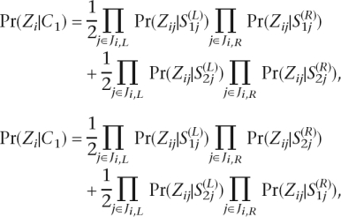By calculating the Pr(Z|C₁) and Pr(Z|C₂), we determine the phase according to the following decision rule:

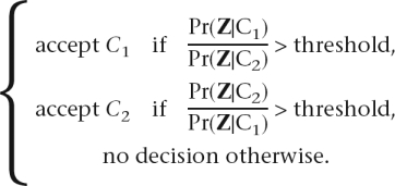The value of the threshold should be >1 (we used 100 in our simulations).

References

- Altschul S.F., Madden T.L., Schaffer A.A., Zhang J., Zhang Z., Miller W., Lipman D.J., Madden T.L., Schaffer A.A., Zhang J., Zhang Z., Miller W., Lipman D.J., Schaffer A.A., Zhang J., Zhang Z., Miller W., Lipman D.J., Zhang J., Zhang Z., Miller W., Lipman D.J., Zhang Z., Miller W., Lipman D.J., Miller W., Lipman D.J., Lipman D.J. Gapped BLAST and PSI-BLAST: A new generation of protein database search program. Nucleic Acids Res. 1997;25:3389–3402. doi: 10.1093/nar/25.17.3389. [DOI] [PMC free article] [PubMed] [Google Scholar]
- Altshuler D., Pollara V.J., Cowles C.R., Van Etten W.J., Baldwin J., Linton L., Lander E.S., Pollara V.J., Cowles C.R., Van Etten W.J., Baldwin J., Linton L., Lander E.S., Cowles C.R., Van Etten W.J., Baldwin J., Linton L., Lander E.S., Van Etten W.J., Baldwin J., Linton L., Lander E.S., Baldwin J., Linton L., Lander E.S., Linton L., Lander E.S., Lander E.S. An SNP map of the human genome generated by reduced representation shotgun sequencing. Nature. 2000;407:513–516. doi: 10.1038/35035083. [DOI] [PubMed] [Google Scholar]
- Aparicio S., Chapman J., Stupka E., Putnam N., Chia J.M., Dehal P., Christoffels A., Rash S., Hoon S., Smit A., Chapman J., Stupka E., Putnam N., Chia J.M., Dehal P., Christoffels A., Rash S., Hoon S., Smit A., Stupka E., Putnam N., Chia J.M., Dehal P., Christoffels A., Rash S., Hoon S., Smit A., Putnam N., Chia J.M., Dehal P., Christoffels A., Rash S., Hoon S., Smit A., Chia J.M., Dehal P., Christoffels A., Rash S., Hoon S., Smit A., Dehal P., Christoffels A., Rash S., Hoon S., Smit A., Christoffels A., Rash S., Hoon S., Smit A., Rash S., Hoon S., Smit A., Hoon S., Smit A., Smit A., et al. Whole-genome shotgun assembly and analysis of the genome of Fugu rubripes. Science. 2002;297:1301–1310. doi: 10.1126/science.1072104. [DOI] [PubMed] [Google Scholar]
- Bafna V., Gusfield D., Lancia G., Yooseph S., Gusfield D., Lancia G., Yooseph S., Lancia G., Yooseph S., Yooseph S. Haplotying as perfect phylogeny: A direct approach. J. Comput. Biol. 2003;10:323–340. doi: 10.1089/10665270360688048. [DOI] [PubMed] [Google Scholar]
- Batzoglou S., Jaffe D.B., Stanley K., Butler J., Gnerre S., Mauceli E., Berger B., Mesirov J.P., Lander E.S., Jaffe D.B., Stanley K., Butler J., Gnerre S., Mauceli E., Berger B., Mesirov J.P., Lander E.S., Stanley K., Butler J., Gnerre S., Mauceli E., Berger B., Mesirov J.P., Lander E.S., Butler J., Gnerre S., Mauceli E., Berger B., Mesirov J.P., Lander E.S., Gnerre S., Mauceli E., Berger B., Mesirov J.P., Lander E.S., Mauceli E., Berger B., Mesirov J.P., Lander E.S., Berger B., Mesirov J.P., Lander E.S., Mesirov J.P., Lander E.S., Lander E.S. ARACHNE: A whole-genome shotgun assembler. Genome Res. 2002;12:177–189. doi: 10.1101/gr.208902. [DOI] [PMC free article] [PubMed] [Google Scholar]
- Bejerano G., Pheasant M., Makunin I., Stephen S., Kent W.J., Mattick J.S., Haussler D., Pheasant M., Makunin I., Stephen S., Kent W.J., Mattick J.S., Haussler D., Makunin I., Stephen S., Kent W.J., Mattick J.S., Haussler D., Stephen S., Kent W.J., Mattick J.S., Haussler D., Kent W.J., Mattick J.S., Haussler D., Mattick J.S., Haussler D., Haussler D. Ultraconserved elements in the human genome. Science. 2004;304:1321–1325. doi: 10.1126/science.1098119. [DOI] [PubMed] [Google Scholar]
- Chen X., Livak K.J., Kwok P.Y., Livak K.J., Kwok P.Y., Kwok P.Y. A homogeneous, ligase-mediated DNA diagnostic test. Genome Res. 1998;8:549–556. doi: 10.1101/gr.8.5.549. [DOI] [PMC free article] [PubMed] [Google Scholar]
- Chou H.H., Holmes M.H., Holmes M.H. DNA sequence quality trimming and vector removal. Bioinformatics. 2001;17:1093–1104. doi: 10.1093/bioinformatics/17.12.1093. [DOI] [PubMed] [Google Scholar]
- Churchill G.A., Waterman M.S., Waterman M.S. The accuracy of DNA sequence: Estimating sequence quality. Genomics. 1992;14:89–98. doi: 10.1016/s0888-7543(05)80288-5. [DOI] [PubMed] [Google Scholar]
- Clark A. Inference of haplotypes from PCR-amplified samples of diploid populations. Mol. Biol. Evol. 1990;7:111–122. doi: 10.1093/oxfordjournals.molbev.a040591. [DOI] [PubMed] [Google Scholar]
- Daly M., Rioux J.D., Schaffner S.F., Hudson T.J., Lander E.S., Rioux J.D., Schaffner S.F., Hudson T.J., Lander E.S., Schaffner S.F., Hudson T.J., Lander E.S., Hudson T.J., Lander E.S., Lander E.S. High-resolution haplotype structure in the human genome. Nat. Genet. 2001;29:229–232. doi: 10.1038/ng1001-229. [DOI] [PubMed] [Google Scholar]
- Dehal P., Satou Y., Campbell R.K., Chapman J., Degnan B., Tomaso A.D., Davidson B., Gregorio A.D., Gelpke M., Goodstein D.M., Satou Y., Campbell R.K., Chapman J., Degnan B., Tomaso A.D., Davidson B., Gregorio A.D., Gelpke M., Goodstein D.M., Campbell R.K., Chapman J., Degnan B., Tomaso A.D., Davidson B., Gregorio A.D., Gelpke M., Goodstein D.M., Chapman J., Degnan B., Tomaso A.D., Davidson B., Gregorio A.D., Gelpke M., Goodstein D.M., Degnan B., Tomaso A.D., Davidson B., Gregorio A.D., Gelpke M., Goodstein D.M., Tomaso A.D., Davidson B., Gregorio A.D., Gelpke M., Goodstein D.M., Davidson B., Gregorio A.D., Gelpke M., Goodstein D.M., Gregorio A.D., Gelpke M., Goodstein D.M., Gelpke M., Goodstein D.M., Goodstein D.M., et al. The draft genome of Ciona intestinalis: Insights into chordate and vertebrate origins. Science. 2002;298:2157–2167. doi: 10.1126/science.1080049. [DOI] [PubMed] [Google Scholar]
- Dermitzakis E.T., Reymond A., Lyle R., Scamuffa N., Ucla C., Deutsch S., Stevenson B.J., Flege V., Bucher P., Jongeneel C.V., Reymond A., Lyle R., Scamuffa N., Ucla C., Deutsch S., Stevenson B.J., Flege V., Bucher P., Jongeneel C.V., Lyle R., Scamuffa N., Ucla C., Deutsch S., Stevenson B.J., Flege V., Bucher P., Jongeneel C.V., Scamuffa N., Ucla C., Deutsch S., Stevenson B.J., Flege V., Bucher P., Jongeneel C.V., Ucla C., Deutsch S., Stevenson B.J., Flege V., Bucher P., Jongeneel C.V., Deutsch S., Stevenson B.J., Flege V., Bucher P., Jongeneel C.V., Stevenson B.J., Flege V., Bucher P., Jongeneel C.V., Flege V., Bucher P., Jongeneel C.V., Bucher P., Jongeneel C.V., Jongeneel C.V., et al. Numerous potentially functional but non-genic conserved sequences on human chromosome 21. Nature. 2002;420:578–582. doi: 10.1038/nature01251. [DOI] [PubMed] [Google Scholar]
- Drysdale C., McGraw D.W., Stack C.B., Stephens J.C., Judson R.S., Nandabalan K., Arnold K., Ruano G., Liggett S.B., McGraw D.W., Stack C.B., Stephens J.C., Judson R.S., Nandabalan K., Arnold K., Ruano G., Liggett S.B., Stack C.B., Stephens J.C., Judson R.S., Nandabalan K., Arnold K., Ruano G., Liggett S.B., Stephens J.C., Judson R.S., Nandabalan K., Arnold K., Ruano G., Liggett S.B., Judson R.S., Nandabalan K., Arnold K., Ruano G., Liggett S.B., Nandabalan K., Arnold K., Ruano G., Liggett S.B., Arnold K., Ruano G., Liggett S.B., Ruano G., Liggett S.B., Liggett S.B. Complex Promoter and coding region β2-adrenergic receptor haplotypes alter receptor expression and predict in vivo responsiveness. Proc. Natl. Acad. Sci. 2000;97:10483–10488. doi: 10.1073/pnas.97.19.10483. [DOI] [PMC free article] [PubMed] [Google Scholar]
- Ewing B., Green P., Green P. Basecalling of automated sequencer traces using Phred. II. error probabilities. Genome Res. 1998;8:186–194. [PubMed] [Google Scholar]
- Excoffier L., Slatkin M., Slatkin M. Maximum-likelihood estimation of molecular haplotype frequencies in a diploid population. Mol. Biol. Evol. 1995;12:921–927. doi: 10.1093/oxfordjournals.molbev.a040269. [DOI] [PubMed] [Google Scholar]
- Halperin E., Eskin E., Eskin E. Haplotype reconstruction from genotype data using imperfect phylogeny. Bioinformatics. 2004;20:1842–1849. doi: 10.1093/bioinformatics/bth149. [DOI] [PubMed] [Google Scholar]
- Hawley M., Kidd K., Kidd K. Haplo: A program using the EM algorithm to estimate the frequencies of multi-site haplotypes. J. Hered. 1995;86:409–411. doi: 10.1093/oxfordjournals.jhered.a111613. [DOI] [PubMed] [Google Scholar]
- Huelsenbeck J.P., Nielsen R., Nielsen R. Effect of Nonindependent substitution on phylogenetic accuracy. Syst. Biol. 1999;48:317–328. doi: 10.1080/106351599260319. [DOI] [PubMed] [Google Scholar]
- Istrail S., Sutton G.G., Florea L., Halpern A., Mobarry C.M., Lippert R., Walenz B., Shatkay H., Dew I., Miller J.R., Sutton G.G., Florea L., Halpern A., Mobarry C.M., Lippert R., Walenz B., Shatkay H., Dew I., Miller J.R., Florea L., Halpern A., Mobarry C.M., Lippert R., Walenz B., Shatkay H., Dew I., Miller J.R., Halpern A., Mobarry C.M., Lippert R., Walenz B., Shatkay H., Dew I., Miller J.R., Mobarry C.M., Lippert R., Walenz B., Shatkay H., Dew I., Miller J.R., Lippert R., Walenz B., Shatkay H., Dew I., Miller J.R., Walenz B., Shatkay H., Dew I., Miller J.R., Shatkay H., Dew I., Miller J.R., Dew I., Miller J.R., Miller J.R., et al. Whole-genome shotgun assembly and comparison of human genome assemblies. Proc. Natl. Acad. Sci. 2004;101:1916–1921. doi: 10.1073/pnas.0307971100. [DOI] [PMC free article] [PubMed] [Google Scholar]
- Jaffe D.B., Butler J., Gnerre S., Mauceli E., Lindblad-Toh K., Mesirov J.P., Zody M.C., Lander E.S., Butler J., Gnerre S., Mauceli E., Lindblad-Toh K., Mesirov J.P., Zody M.C., Lander E.S., Gnerre S., Mauceli E., Lindblad-Toh K., Mesirov J.P., Zody M.C., Lander E.S., Mauceli E., Lindblad-Toh K., Mesirov J.P., Zody M.C., Lander E.S., Lindblad-Toh K., Mesirov J.P., Zody M.C., Lander E.S., Mesirov J.P., Zody M.C., Lander E.S., Zody M.C., Lander E.S., Lander E.S. Whole-genome sequence assembly for mammalian genomes: Arachne 2. Genome Res. 2003;13:91–96. doi: 10.1101/gr.828403. [DOI] [PMC free article] [PubMed] [Google Scholar]
- Johnson D.S., Davidson B., Brown C.D., Smith W.C., Sidow A., Davidson B., Brown C.D., Smith W.C., Sidow A., Brown C.D., Smith W.C., Sidow A., Smith W.C., Sidow A., Sidow A. Noncoding regulatory sequences of Ciona exhibit strong correspondence between evolutionary constraint and functional importance. Genome Res. 2004;14:2448–2456. doi: 10.1101/gr.2964504. [DOI] [PMC free article] [PubMed] [Google Scholar]
- Jones T., Federspiel N.A., Chibana H., Dungan J., Kalman S., Magee B.B., Newport G., Thorstenson Y.R., Agabian N., Magee P.T., Federspiel N.A., Chibana H., Dungan J., Kalman S., Magee B.B., Newport G., Thorstenson Y.R., Agabian N., Magee P.T., Chibana H., Dungan J., Kalman S., Magee B.B., Newport G., Thorstenson Y.R., Agabian N., Magee P.T., Dungan J., Kalman S., Magee B.B., Newport G., Thorstenson Y.R., Agabian N., Magee P.T., Kalman S., Magee B.B., Newport G., Thorstenson Y.R., Agabian N., Magee P.T., Magee B.B., Newport G., Thorstenson Y.R., Agabian N., Magee P.T., Newport G., Thorstenson Y.R., Agabian N., Magee P.T., Thorstenson Y.R., Agabian N., Magee P.T., Agabian N., Magee P.T., Magee P.T., et al. The diploid genome sequence of Candida albicans. Proc. Natl. Acad. Sci. 2004;101:7329–7334. doi: 10.1073/pnas.0401648101. [DOI] [PMC free article] [PubMed] [Google Scholar]
- Kent J.W. BLAT—The BLAST-like alignment tool. Genome Res. 2002;12:656–664. doi: 10.1101/gr.229202. [DOI] [PMC free article] [PubMed] [Google Scholar]
- Kim J.H., Waterman M.S., Li L.M., Waterman M.S., Li L.M., Li L.M. Accuracy assessment of diploid consensus sequences. IEEE/ACM Trans. Comput. Biol. Bioinform. 2007;4:88–97. doi: 10.1109/TCBB.2007.1007. [DOI] [PubMed] [Google Scholar]
- Kurtz S., Phillippy A., Delcher A.L., Smoot M., Shumway M., Antonescu C., Salzberg S.L., Phillippy A., Delcher A.L., Smoot M., Shumway M., Antonescu C., Salzberg S.L., Delcher A.L., Smoot M., Shumway M., Antonescu C., Salzberg S.L., Smoot M., Shumway M., Antonescu C., Salzberg S.L., Shumway M., Antonescu C., Salzberg S.L., Antonescu C., Salzberg S.L., Salzberg S.L. Versatile and open software for comparing large genomes. Genome Biol. 2004;5:R12. doi: 10.1186/gb-2004-5-2-r12. [DOI] [PMC free article] [PubMed] [Google Scholar]
- Lancia G., Bafna V., Istrail S., Lippert R., Schwartz R., Bafna V., Istrail S., Lippert R., Schwartz R., Istrail S., Lippert R., Schwartz R., Lippert R., Schwartz R., Schwartz R. Lecture Notes in Computer Science. Springer; Berlin: 2001. SNPs problems, complexity, and algorithms; pp. 182–193. Vol. 2161. [Google Scholar]
- Lander E.S., Linton L.M., Birren B., Nusbaum C., Zody M.C., Baldwin J., Devon K., Dewar K., Doyle M., FitzHugh W., Linton L.M., Birren B., Nusbaum C., Zody M.C., Baldwin J., Devon K., Dewar K., Doyle M., FitzHugh W., Birren B., Nusbaum C., Zody M.C., Baldwin J., Devon K., Dewar K., Doyle M., FitzHugh W., Nusbaum C., Zody M.C., Baldwin J., Devon K., Dewar K., Doyle M., FitzHugh W., Zody M.C., Baldwin J., Devon K., Dewar K., Doyle M., FitzHugh W., Baldwin J., Devon K., Dewar K., Doyle M., FitzHugh W., Devon K., Dewar K., Doyle M., FitzHugh W., Dewar K., Doyle M., FitzHugh W., Doyle M., FitzHugh W., FitzHugh W., et al. Initial sequencing and analysis of the human genome. Nature. 2001;409:860–921. doi: 10.1038/35057062. [DOI] [PubMed] [Google Scholar]
- Li L.M., Kim J.H., Waterman M.S., Kim J.H., Waterman M.S., Waterman M.S. Haplotype reconstruction from SNP alignment. J. Comput. Biol. 2004;11:505–516. doi: 10.1089/1066527041410454. [DOI] [PubMed] [Google Scholar]
- Liu J.S. Monte Carlo strategies in scientific computing. Springer-Verlag; New York: 2002. [Google Scholar]
- Long J., Williams R., Urbanek M., Williams R., Urbanek M., Urbanek M. An E-M algorithm and testing strategy for multiple-locus haplotypes. Am. J. Hum. Genet. 1995;56:799–810. [PMC free article] [PubMed] [Google Scholar]
- Mikkelsen T.S., Hillier L.W., Eichler E.E., Zody M.C., Jaffe D.B., Yang S., Enard W., Hellmann I., Lindblad-Toh K., Altheide T.K., Hillier L.W., Eichler E.E., Zody M.C., Jaffe D.B., Yang S., Enard W., Hellmann I., Lindblad-Toh K., Altheide T.K., Eichler E.E., Zody M.C., Jaffe D.B., Yang S., Enard W., Hellmann I., Lindblad-Toh K., Altheide T.K., Zody M.C., Jaffe D.B., Yang S., Enard W., Hellmann I., Lindblad-Toh K., Altheide T.K., Jaffe D.B., Yang S., Enard W., Hellmann I., Lindblad-Toh K., Altheide T.K., Yang S., Enard W., Hellmann I., Lindblad-Toh K., Altheide T.K., Enard W., Hellmann I., Lindblad-Toh K., Altheide T.K., Hellmann I., Lindblad-Toh K., Altheide T.K., Lindblad-Toh K., Altheide T.K., Altheide T.K., et al. Initial sequence of the chimpanzee genome and comparison with the human genome. Nature. 2005;437:69–87. doi: 10.1038/nature04072. [DOI] [PubMed] [Google Scholar]
- Niu T., Qin Z.S., Xu X., Liu J.S., Qin Z.S., Xu X., Liu J.S., Xu X., Liu J.S., Liu J.S. Bayesian haplotype inference for multiple linked single-nucleotide polymorphisms. Am. J. Hum. Genet. 2002;70:157–169. doi: 10.1086/338446. [DOI] [PMC free article] [PubMed] [Google Scholar]
- Nobrega M.A., Zhu Y., Plajzer-Frick I., Afzal V., Rubin E.M., Zhu Y., Plajzer-Frick I., Afzal V., Rubin E.M., Plajzer-Frick I., Afzal V., Rubin E.M., Afzal V., Rubin E.M., Rubin E.M. Megabase deletions of gene deserts result in viable mice. Nature. 2004;431:988–993. doi: 10.1038/nature03022. [DOI] [PubMed] [Google Scholar]
- Nordborg M. Coalescent theory. In: Bishop D.M., Cannings C., Cannings C., editors. Handbook of statistical genetics. Wiley; Chichester, UK: 2001. Chapter 7. [Google Scholar]
- Pastinen T., Kurg A., Metspalu A., Peltonen L., Syvanen A.C., Kurg A., Metspalu A., Peltonen L., Syvanen A.C., Metspalu A., Peltonen L., Syvanen A.C., Peltonen L., Syvanen A.C., Syvanen A.C. Minisequencing: A specific tool for DNA analysis and diagnostics on oligonucleotide arrays. Genome Res. 1997;7:606–614. doi: 10.1101/gr.7.6.606. [DOI] [PubMed] [Google Scholar]
- Siepel A., Bejerano G., Pedersen J.S., Hinrichs A.S., Hou M., Rosenbloom K., Clawson H., Spieth J., Hillier L.W., Richards S., Bejerano G., Pedersen J.S., Hinrichs A.S., Hou M., Rosenbloom K., Clawson H., Spieth J., Hillier L.W., Richards S., Pedersen J.S., Hinrichs A.S., Hou M., Rosenbloom K., Clawson H., Spieth J., Hillier L.W., Richards S., Hinrichs A.S., Hou M., Rosenbloom K., Clawson H., Spieth J., Hillier L.W., Richards S., Hou M., Rosenbloom K., Clawson H., Spieth J., Hillier L.W., Richards S., Rosenbloom K., Clawson H., Spieth J., Hillier L.W., Richards S., Clawson H., Spieth J., Hillier L.W., Richards S., Spieth J., Hillier L.W., Richards S., Hillier L.W., Richards S., Richards S., et al. Evolutionarily conserved elements in vertebrate, insect, worm, and yeast genomes. Genome Res. 2005;15:1034–1050. doi: 10.1101/gr.3715005. [DOI] [PMC free article] [PubMed] [Google Scholar]
- Stephens M., Smith N.J., Donnelly P., Smith N.J., Donnelly P., Donnelly P. A new statistical method for haplotype reconstruction from population data. Am. J. Hum. Genet. 2001;68:978–989. doi: 10.1086/319501. [DOI] [PMC free article] [PubMed] [Google Scholar]
- Taillon-Miller P., Gu Z., Li Q., Hillier L., Kwok P.Y., Gu Z., Li Q., Hillier L., Kwok P.Y., Li Q., Hillier L., Kwok P.Y., Hillier L., Kwok P.Y., Kwok P.Y. Overlapping genomic sequences: A treasure trove of single-nucleotide polymorphisms. Genome Res. 1998;8:748–754. doi: 10.1101/gr.8.7.748. [DOI] [PMC free article] [PubMed] [Google Scholar]
- Venter J.C., Adams M.D., Myers E.W., Li P.W., Mural R.J., Sutton G.G., Smith H.O., Yandell M., Evans C.A., Holt R.A., Adams M.D., Myers E.W., Li P.W., Mural R.J., Sutton G.G., Smith H.O., Yandell M., Evans C.A., Holt R.A., Myers E.W., Li P.W., Mural R.J., Sutton G.G., Smith H.O., Yandell M., Evans C.A., Holt R.A., Li P.W., Mural R.J., Sutton G.G., Smith H.O., Yandell M., Evans C.A., Holt R.A., Mural R.J., Sutton G.G., Smith H.O., Yandell M., Evans C.A., Holt R.A., Sutton G.G., Smith H.O., Yandell M., Evans C.A., Holt R.A., Smith H.O., Yandell M., Evans C.A., Holt R.A., Yandell M., Evans C.A., Holt R.A., Evans C.A., Holt R.A., Holt R.A., et al. The sequence of the human genome. Science. 2001;291:1304–1351. doi: 10.1126/science.1058040. [DOI] [PubMed] [Google Scholar]
- Venter J.C., Remington K., Heidelberg J.F., Halpern A.L., Rusch D., Eisen J.A., Wu D., Paulsen I., Nelson K.E., Nelson W., Remington K., Heidelberg J.F., Halpern A.L., Rusch D., Eisen J.A., Wu D., Paulsen I., Nelson K.E., Nelson W., Heidelberg J.F., Halpern A.L., Rusch D., Eisen J.A., Wu D., Paulsen I., Nelson K.E., Nelson W., Halpern A.L., Rusch D., Eisen J.A., Wu D., Paulsen I., Nelson K.E., Nelson W., Rusch D., Eisen J.A., Wu D., Paulsen I., Nelson K.E., Nelson W., Eisen J.A., Wu D., Paulsen I., Nelson K.E., Nelson W., Wu D., Paulsen I., Nelson K.E., Nelson W., Paulsen I., Nelson K.E., Nelson W., Nelson K.E., Nelson W., Nelson W., et al. Environmental genome shotgun sequencing of the Sargasso sea. Science. 2004;304:66–74. doi: 10.1126/science.1093857. [DOI] [PubMed] [Google Scholar]
- Vinson J., Jaffe D.B., O’Neill K., Karlsson E.K., Stange-Thomann N., Anderson S., Mesirov J.P., Satoh N., Satou Y., Nusbaum C., Jaffe D.B., O’Neill K., Karlsson E.K., Stange-Thomann N., Anderson S., Mesirov J.P., Satoh N., Satou Y., Nusbaum C., O’Neill K., Karlsson E.K., Stange-Thomann N., Anderson S., Mesirov J.P., Satoh N., Satou Y., Nusbaum C., Karlsson E.K., Stange-Thomann N., Anderson S., Mesirov J.P., Satoh N., Satou Y., Nusbaum C., Stange-Thomann N., Anderson S., Mesirov J.P., Satoh N., Satou Y., Nusbaum C., Anderson S., Mesirov J.P., Satoh N., Satou Y., Nusbaum C., Mesirov J.P., Satoh N., Satou Y., Nusbaum C., Satoh N., Satou Y., Nusbaum C., Satou Y., Nusbaum C., Nusbaum C., et al. Assembly of polymorphic genomes: Algorithms and application to Ciona savignyi. Genome Res. 2005;15:1127–1135. doi: 10.1101/gr.3722605. [DOI] [PMC free article] [PubMed] [Google Scholar]
- Wang D., Fan J.B., Siao C.J., Berno A., Young P., Sapolsky R., Ghandour G., Perkins N., Winchester E., Spencer J., Fan J.B., Siao C.J., Berno A., Young P., Sapolsky R., Ghandour G., Perkins N., Winchester E., Spencer J., Siao C.J., Berno A., Young P., Sapolsky R., Ghandour G., Perkins N., Winchester E., Spencer J., Berno A., Young P., Sapolsky R., Ghandour G., Perkins N., Winchester E., Spencer J., Young P., Sapolsky R., Ghandour G., Perkins N., Winchester E., Spencer J., Sapolsky R., Ghandour G., Perkins N., Winchester E., Spencer J., Ghandour G., Perkins N., Winchester E., Spencer J., Perkins N., Winchester E., Spencer J., Winchester E., Spencer J., Spencer J., et al. Large-scale identification, mapping, and genotyping of single-nucleotide polymorphisms in the human genome. Science. 1998;280:1077–1082. doi: 10.1126/science.280.5366.1077. [DOI] [PubMed] [Google Scholar]