MinActionPath: maximum likelihood trajectory for large-scale structural transitions in a coarse-grained locally harmonic energy landscape

Abstract

The non-linear problem of simulating the structural transition between two known forms of a macromolecule still remains a challenge in structural biology. The problem is usually addressed in an approximate way using ‘morphing’ techniques, which are linear interpolations of either the Cartesian or the internal coordinates between the initial and end states, followed by energy minimization. Here we describe a web tool that implements a new method to calculate the most probable trajectory that is exact for harmonic potentials; as an illustration of the method, the classical Calpha-based Elastic Network Model (ENM) is used both for the initial and the final states but other variants of the ENM are also possible. The Langevin equation under this potential is solved analytically using the Onsager and Machlup action minimization formalism on each side of the transition, thus replacing the original non-linear problem by a pair of linear differential equations joined by a non-linear boundary matching condition. The crossover between the two multidimensional energy curves around each state is found numerically using an iterative approach, producing the most probable trajectory and fully characterizing the transition state and its energy. Jobs calculating such trajectories can be submitted on-line at: http://lorentz.dynstr.pasteur.fr/joel/index.php.

INTRODUCTION

Both structural and dynamical properties of macromolecules are essential to understand in order to account for their biological function. There are numerous examples (1) of large-scale and biologically important structural rearrangements in the Protein Data Base (PDB), including allosteric molecules, molecular motors and receptors that undergo a transition from an open to a closed state upon ligand binding (induced fit).

While experimental methods such as X-Ray crystallography can give an atomic description of the two end states, the transition state is inaccessible to such structural methods because it is by nature unstable. NMR might be amenable to give some answers to the dynamical aspects of the transition as shown very recently (2) but such applications will likely be very difficult for large macromolecular systems such as molecular motors.

Yet it would be of tremendous importance to have access to the structural characteristics of such a transition state. Indeed this would open the way to design drugs against transiently formed intermediate structures instead of just the starting or end points of the transition. Also, it would help to understand enzymology at the molecular level, which proceeds through the stabilization of the transition state complex with the substrate(s) (3).

When studying structural transitions, it is important to distinguish between morphing techniques (4), which interpolate linearly between the starting and end states, and reaction path direct determination using physical potentials. Indeed, interpolation techniques will likely fail for large amplitude transitions and a physical description of the transition is to be preferred, if feasible, over a purely geometrical one in all cases.

Simulation techniques such as molecular dynamics (MD) can in principle be used to study such transition in atomic detail, but the time scale accessible to such methods is several orders of magnitude smaller than the time scale during which these phenomena occur in solution. A common strategy then is to resort to coarse-grained models. Among the various existing coarse-grained models, two of them have been intensively studied in the past for structural transitions, namely the elastic network model (ENM) (5) and the Go model (6). While it is clear that ENM has the potential to describe a good part of naturally occurring and documented structural transitions through a handful of low-frequency normal modes derived from this simple model (7) the problem remains that the ENM has by definition only one minimum and is therefore inadequate to describe the full transition. This problem is also present in the Go model, which basically assumes that only native-like contacts can occur during the transition whereas in reality non-native contacts may well appear and disappear in the process.

Recently, several groups have started to address these points through innovative ways, taking into account the double-well character of the energy landscape. The main difficulty with these methods is that they have to make simplifying assumptions in order to locate the crossing points of the two energy surfaces (8–11).

Here we revisit the original Kramers problem (12) of finding the trajectory between two stable states experiencing each a harmonic potential. We use an entirely different method, the so-called Onsager–Machlup method, which reformulates the Langevin equation as an action minimization problem (13). Such an approach has been used recently by several groups to study both peptide (14,15) and protein folding-unfolding transitions (16–19), using classical force fields and numerical simulations. Here we show that by using a normal mode representation we can solve the equations on each side of the transition analytically, i.e. without any approximation; the problem is then narrowed down to finding the crossing point of these two solutions, which is achieved numerically through a one-dimensional search.

We have implemented the technique on a web server that will automatically generate a trajectory between two states provided by the user, given just a few parameters: the energy difference between the two states (usually close to zero or a few kT), the relative spring constants of the harmonic potentials, which can be estimated through a fit with the experimental B-factors, and the cutoff radius of the ENM (typically 10–12 Å).

MATERIALS AND METHODS

We assume that the energy landscape around each state (initial and final) is harmonic. To describe the transition between the two states we must solve the Langevin equation in the following energy landscape:

for the left side of the transition state and

for the right side of the transition state, where Q and P are the Hessians around the initial states X_i and the final state X_f, respectively, and ▵E accounts for a difference in energy between the two states X_i and X_f.

Assuming an overdamped regime and following Onsager and Machlup (13), the stochastic Langevin equation is transformed into a deterministic differential equation by asking for a minimum mechanical action of the form S = ∫ (dX/dt + ∂ V/∂ X)²dt. This leads to:

and

where we require continuity for both positions and velocities at the crossing point t = t₀.

An analytical solution can be found for both the left and right sides using boundary conditions X(t = 0) = X_i and X(t = t₀) = X^#, and X(t = t₀) = X^# and X(t = T) = X_f, respectively, by decomposing both Q and P into eigenstates (normal modes) and solving each mode separately (the null space corresponding to the three overall translations and three overall rotations is treated separately). Continuity of speed dX/dt is also required at the crossing point t₀ to fully specify the analytical solution. An initial guess is made for t₀, which is then progressively refined numerically until U_<(X(t₀)) = U_>(X(t₀)), up to machine precision; we find that this requires the use of all 3N normal modes (Franklin et al., in preparation).

In order to study both a simple and realistic model of the system, we use the ENM based on a C-alpha (CA) representation of the molecule, that captures well collective and large-scale amplitude movements which typically occur in macromolecular transitions (7,20). The Energy thus reads 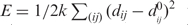where the sum is restricted to those pairs with an inter-atomic distance less than R_c in the ground state (5). The spring constant k, which sets the scale of the energy E, can be taken to be different for the initial state (k_<) and the final state (k_>). Also, it is possible to assign a much stronger elastic constant (100k) for distances involving between consecutive CAs, which should remain at 3.8 Å, except for the rare cis-peptides bonds (21).

Protocol

A typical run of the program consists of the following steps (Figure 1):

1. Extract the CAs atoms from both the initial and final states and superimpose them with Profit (http://www.bioinf.org.uk/software/profit/index.html). For nucleic acids, we would typically use three atoms per nucleotide (P, C1’ and C4’).

2. Fit the experimental B-factors, if they are known, of each form, to the computed <▵r²>, to estimate both k_< and k_>. The default is k_< = k_> = 0.1 kcal/mol/Ų

3. Submit the trajectory job. The only physical parameter remaining to be chosen is ▵E, the energy difference between the two states. In general ▵E is unknown but of the order of a few kcal/mol and can be refined in the following step of the procedure. The length of the simulation T is fixed by the prescription that S_tot has reached a plateau. A few increasing trial values may be necessary to ensure this prescription, which is usually met with T = 150–200. The number of sampling points is arbitrary since the maximum likelihood trajectory is obtained analytically so that one can sample it at any arbitrary set of time snapshots, at the user's convenience.

4. Once a trajectory has been calculated, both S_tot and E^# are examined: S_tot to check for asymptotic behavior and E^# to compare with ▵G^#_exp, if available. Different values of ▵E [step (iii)] can be tried to achieve the desired value of ▵G^#_exp which is related to the observed rate constant of the reaction.

5. Once a satisfactory trajectory has been obtained, all atom models for the transition state and possibly each frame of the trajectory can be reconstructed using online tools. In particular, all atoms can be generated for proteins from CA-only coordinates by first generating backbone atoms using a library of fragments of the PDB of length 4 (22) and then generating all sidechain atoms using the self-consistent Mean Field method (23). This will inevitably deform somewhat the CA positions, usually within 0.5–0.7 Å. The whole procedure can therefore be described as essentially coarse-grained, producing trajectories for CAs only and then building sidechains. This is in line with the description of the dynamics of proteins made earlier by Hinsen and Kneller (24), which they describe as essentially harmonic and where anharmonicity enters in the rigid-body movement of side chains (described here as rotamers).

Figure 1.

Flow chart of the web site. The input consists of two PDB files of one macromolecule in two different conformations, the estimated energy difference between the two states, the ENM cutoff (10–12 Å) and the elastic constants for the two states, which can be estimated on-line. The returned output is the most probable trajectory between the two states (loadable by PyMol) and the coordinates of the transition state, its energy E^# with respect to the initial state and the value of the minimized action S_tot in the trajectory. Insert: One-dimensional representation of the shift on the crossing point of the two harmonic curves when using different energy differences between the two states, and when using an increasing elastic constant for the end state.

One might argue that the reconstruction of all atoms introduces some damage in the continuity of the trajectory. An interpolation technique could be used to restore this continuity, or, alternatively, these snapshots could be used for ‘steered’ MD simulations using harmonic restraints on the CA positions.

RESULTS

We tested the structural transitions studied in (25) for which the root mean square distance (rmsd) between the two forms is in the range of 3.0 Å to 15 Å. In all cases the algorithm produced a solution that was subsequently checked visually using PyMol (http://www.pymol.org) or VMD (www.ks.uiuc.edu/Research/vmd) and with a post-processing program that showed they were satisfying both in terms of the absence of steric clashes and of the small deviation of consecutive CA–CA bond lengths around the ideal value of 3.8 Å (Table 1). This allowed in all cases the reconstruction of all atom models for the transition states. The largest computation was performed on citrate synthase, a dimer of 852 CA atoms, for which it takes about 2 h c.p.u. time on a 2.8 GHz Pentium IV Linux workstation. The same computation takes about 1 min for calmodulin (138 residues). We do not recommend submitting jobs with files containing more than 1000 atoms. A couple of transitions were taken from (20), in order to have a representative set of protein sizes: this allowed to determine the power law of the c.p.u. time as a function of size namely O(N^3.6).

Table 1.

Structural transitions for which a path has been calculated (20,25)

Name	PDB	Rmsd (Angstrom)	# aa	C.p.u. (mn)	d(i, i + 1) trans. state
Calmodulin	1K9K	4.52	89	<1	4.05 (0.55)
	1K9P
Calmodulin	1CTR	15	138	1	4.66 (0.93)
	1CLL
Dihydrofolate reductase	1RX2	1.22	160	1	3.80 (0.09)
	1RX6
T4	178L	3.45	162	1	3.80 (0.11)
lysozyme	256L
Adenylate kinase	4AKE	7.1	214	2	3.97 (0.19)
	1AKE
Glutamine binding	1GGG	5.3	225	2	3.87 (0.21)
	1WDN
Ornithine binding	2LAO	4.7	242	2	3.87 (0.16)
	1LST
DNA Pol	1BPX	2.8	326	6	3.78 (0.12)
beta	1BPY
Maltodextrin binding	1ANF	3.8	370	9	3.86 (0.126)
	1OMP
Pol I	3KTQ	1.96	528	27	3.84 (0.36)
Taq	2KTQ
Pol I	1L3V	2.06	580	35	3.82 (0.12)
Bacillus	1LV5
Lactoferrin	1LFG	4.7	691	76	3.87 (0.16)
	1CB6
Citrate synthase	5CSC	3	852	160	3.84 (0.21)
	6CSC

Particularly impressive was the ability of the program to generate a continuous trajectory for calmodulin (in which case the rmsd between the final and initial states is 15 Å), for which a morphing technique (26) that interpolates all intramolecular distances within R_c and recently implemented on a web server by both this group (27) and ours (28) required adjusting R_c by trial and error. Due to the large-scale character of the transition, calmodulin displayed the largest deviations of CA–CA distances but this did not prevent reconstruction of all atoms.

We now discuss in more detail the case of adenylate kinase (rmsd of 7.1 Å between final and initial state), which is a widely used and studied example of an induced-fit mechanism in the field of simulating structural transitions (8,10,11). We, as others, observe that the closure of the LID domain occurs first and is nearly completed once the rearrangement of the catalytic domain begins. The transition state is located near the end of the LID domain closure. This may be related to the observation that a few low-frequency normal modes suffice to describe the closure of the LID (25). There has been some speculation that the transition is accompanied by unfolding and ‘cracking’ due to the accumulation of elastic strain at some points in the trajectory (10,11). Note, however, that we use all 3N normal modes to describe the transition, not just a handful of low-frequency ones (10,11). To test this strain and cracking hypothesis we calculated a Q1 vs Q2 plot for this transition, where Q(t) measures the fraction of native contacts at time t along the trajectory, defined as pairs of atoms with d_ij<R_c, and where the index 1 or 2 refers to the state that is considered as ‘native’: 1 for the initial state and 2 for the final state (Figure 2). We observe a clear decrease in Q1 in the first phase while the increase in Q2 occurs in the very last steps of the trajectory, once the transition state barrier has been overcome. The plot clearly demonstrates the non-linear character of the trajectory generated by our method. The same kind of plot is also shown for the UMMS method of Kim and colleagues (26,27), which always wanders around the straight line joining state 1 (Q1(1) = 1, Q2(1)<1) to state 2 (Q1(2)<1, Q2(2) = 1), by construction. On the contrary, the present method will avoid high-energy regions and depart markedly from this kind of linear trajectory. This is also demonstrated in the energy plot of the transition path for both our method and the UMMS method (Supplementary Figure S1), which clearly shows that elastic energy is much better in our case.

Figure 2.

Q1 versus Q2 plot for adenylate kinase transition (4AKE and 1AKE). Q1 (resp. Q2) is the fraction of native contacts (d_ij < R_c) as in the initial form (resp. in the final form). The trajectory is identical, within machine precision, if one exchanges the role of the initial and final states. For comparison, the same plot is drawn for a trajectory generated according to UMMS (26,27).

Another possibility is to plot Q’1(t)–Q’2(t) versus Q_common(t), i.e. the difference of the number of contacts specific to each state vs the number of contacts seen in both states, for each snapshot (9,11). It is then seen that only about 5% of the common contacts are temporarily lost during the transition (Supplementary Figure S2).

Finally, because the calculation is very rapid for adenylate kinase, it is even possible to screen the effect of mutations of each residue on the kinetics of the transition: for each residue, in turn, we assign a different elastic constant (10k) describing its interactions with its neighbors, and we report the transition state energy of the calculated trajectory (Supplementary Figure S3). This is a new application analogous to the phi-values in protein folding studies, allowing direct comparison with experiments.

DISCUSSION

There exists several variants of the ENM that have also been implemented by us, namely (i) the chemical bond model (21), to take care of possible outliers in CA–CA bond distances and (ii) a distance-dependent weighting scheme for the spring constant as in Hinsen (29), who used 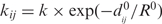or Bahar and colleagues (30), who used 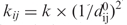. This has the effect of putting more constraints to short distances, which are the most critical ones (they should never come close to zero). Also, one must mention the fact that the Langevin equation used here has constant atomic friction coefficients (set to unity); one way to use more realistic environment-dependent friction coefficients is described in (24) and has also been implemented by us, with qualitatively little effect on the trajectory. The robustness of the trajectory with respect to systematic variations of the k_</k_> ratio, on one hand, or ▵E, on the other hand, has been checked (Supplementary Figures S4 and S5).

The method works if the harmonic approximation for the energy landscape around each state is valid. It would not make any sense to generate a trajectory between two states when it is known that there is an obligatory intermediate state, just to see if this intermediate shows up during the simulation; indeed, in this case, the harmonic approximation would not be valid any more. However, we note that the method can easily be generalized to an energy landscape with three harmonic wells, leading to a search for t₀ to be conducted in a plane instead of a line.

The procedure presented here is quite general, and not limited to proteins. In particular, we are interested in looking at structural transitions occurring in nucleic acids, both DNA and RNA. In both cases however, we still need a method for generating a full atom model based on a coarse representation of the molecule (for example, only including P, C4’ and C1’ atoms for each base). We are currently working on this problem.

CONCLUSION AND FUTURE WORK

In summary, we have presented a new method that combines the action minimization formalism and the ENM to generate trajectories between two known structural states of a given macromolecule. The method is exact if each state is experiencing a harmonic potential and, contrary to other similar methods, does not resort to numerical optimization methods such as Monte Carlo or simulated annealing. It was tested on a large test set of large amplitude structural rearrangements, involving rmsds between the two forms of up to 15 Å. Extensive comparisons with other methods were done in the case of adenylate kinase, which is the most documented example in this field, leading to the systematic use of Q1 versus Q2 plots to characterize the transition.

More tests and comparisons with experimental results will be necessary to assess further the usefulness of the method. This will be made possible by the present web server, which allows experimentalists to look at possible scenarios that can be easily visualized and checked with PyMol or VMD for the structural transition they are interested in.

We are planning to extend the method to the simulation of a transition driven by an applied force (Franklin et al., in preparation), for which direct comparison with single-molecule experiments will then be made possible.

SUPPLEMENTARY DATA

Supplementary Data are available at NAR Online.

REFERENCES

- 1.Flores S, Echols E, Milburn D, Hespenheide B, Keating K, Lu J, Wells S, Yu EZ, Thorpe M, et al. The Database of Macromolecular Motions: new features added at the decade mark. Nucleic Acids Res. 2006;34:D296–D301. doi: 10.1093/nar/gkj046. [DOI] [PMC free article] [PubMed] [Google Scholar]
- 2.Boehr DD, McElhenny D, Dyson HJ, Wright PE. The dynamic energy landscape of dihydrofolate reductase catalysis. Science. 2006;313:1638–1642. doi: 10.1126/science.1130258. [DOI] [PubMed] [Google Scholar]
- 3.Jencks WP. Catalysis in Chemistry and Biology. New York: Dover Publications; 1987. [Google Scholar]
- 4.Krebs WG, Gerstein M. The Morph Server: a standardized system for analyzing and visualizing macromolecular motions in a database framework. Nucleic Acids Res. 2000;28:1665–1675. doi: 10.1093/nar/28.8.1665. [DOI] [PMC free article] [PubMed] [Google Scholar]
- 5.Tirion M. Large amplitude elastic motions in proteins from a single parameter, atomic analyses. Phys. Rev. Lett. 1996;77:1905–1908. doi: 10.1103/PhysRevLett.77.1905. [DOI] [PubMed] [Google Scholar]
- 6.Go N. Theoretical studies of protein folding. Annu. Rev. Biophys. Bioeng. 1983;12:183–210. doi: 10.1146/annurev.bb.12.060183.001151. [DOI] [PubMed] [Google Scholar]
- 7.Krebs WG, Alexandrov V, Wilson CA, Echols N, Yu H, Gerstein M. Normal mode analysis of macromolecular motions in a database framework: developing mode concentration as a useful classifying statistic. Proteins. 2002;48:682–695. doi: 10.1002/prot.10168. [DOI] [PubMed] [Google Scholar]
- 8.Maragakis P, Karplus M. Large amplitude conformational change in proteins explored with a plastic network model: adenylate kinase. J. Mol. Biol. 2005;352:807–822. doi: 10.1016/j.jmb.2005.07.031. [DOI] [PubMed] [Google Scholar]
- 9.Best RB, Chen YG, Hummer G. Slow protein conformational dynamics from multiple experimental structures: the helix/sheet transition of Arc Repressor. Structure. 2005;13:1755–1763. doi: 10.1016/j.str.2005.08.009. [DOI] [PubMed] [Google Scholar]
- 10.Miyashita O, Onuchic JN, Wolynes PG. Nonlinear elasticity, proteinquakes and the energy landscapes of functional transitions in proteins. Proc. Natl Acad. Sci. (USA) 2003;100:12570–575. doi: 10.1073/pnas.2135471100. [DOI] [PMC free article] [PubMed] [Google Scholar]
- 11.Okazaki KI, Koga N, Takada S, Onuchic JN, Wolynes PG. Multiple-basin energy-landscapes for large-amplitude conformational motions of proteins: structure-based molecular dynamics simulations. Proc. Natl Acad. Sci. (USA) 2006;103:11844–11849. doi: 10.1073/pnas.0604375103. [DOI] [PMC free article] [PubMed] [Google Scholar]
- 12.Kramers H. Transition state theory. Physica. 1940;7:284. [Google Scholar]
- 13.Onsager L, Machlup S. Fluctuations and irreversible processes. Phys. Rev. 1953;91:1505–1512. [Google Scholar]
- 14.Cardenas AE, Elber R. Atomically detailed simulations of helix formation with the stochastic difference equation. Biophys. J. 2003;85:2919–2939. doi: 10.1016/S0006-3495(03)74713-4. [DOI] [PMC free article] [PubMed] [Google Scholar]
- 15.Lipfert I, Franklin J, Wu F, Doniach S. Protein misfolding and amyloid formation for the peptide GNNQQNY from yeast prion protein Sup35: simulation by reaction path annealing. J. Mol. Biol. 2005;349:648–658. doi: 10.1016/j.jmb.2005.03.083. [DOI] [PubMed] [Google Scholar]
- 16.Eastman P, Gronbech-Jensen N, Doniach S. Simulation of protein folding by reaction path annealing. J. Chem. Phys. 2001;114:3823–3841. [Google Scholar]
- 17.Ghosh A, Elber R, Scheraga HA. An atomically detailed study of the folding pathways of protein A with the stochastic difference equation. Proc. Natl Acad. Sci. (USA) 2002;99:10394–10398. doi: 10.1073/pnas.142288099. [DOI] [PMC free article] [PubMed] [Google Scholar]
- 18.Wang J, Zhang K, Lu H, Wang E. Quantifying kinetic paths of protein folding. Biophys. J. 2005;89:1612–1620. doi: 10.1529/biophysj.104.055186. [DOI] [PMC free article] [PubMed] [Google Scholar]
- 19.Faccioli P, Sega M, Pederiva F, Orland H. Dominant pathways in protein folding. Phys. Rev. Lett. 2006;97:108101. doi: 10.1103/PhysRevLett.97.108101. [DOI] [PubMed] [Google Scholar]
- 20.Delarue M, Sanejouand YH. Normal mode analysis of conformational transitions in DNA-dependent polymerases: the elastic network model. J. Mol. Biol. 2002;320:1011–1024. doi: 10.1016/s0022-2836(02)00562-4. [DOI] [PubMed] [Google Scholar]
- 21.Kondrashov DA, Cui Q, Phillips GN., Jr Optimization and evaluation of a coarse-grained model of protein motion using X-Ray crystal data. Biophys. J. 2006;91:2760–2767. doi: 10.1529/biophysj.106.085894. [DOI] [PMC free article] [PubMed] [Google Scholar]
- 22.Kolodny R, Koehl P, Guibes L, Levitt M. Small libraries of protein fragments model native protein structures accurately traces. J. Mol. Biol. 2002;323:297–307. doi: 10.1016/s0022-2836(02)00942-7. [DOI] [PubMed] [Google Scholar]
- 23.Koehl P, Delarue M. Application of a self-consistent mean field theory to predict protein side chain conformations and estimate their entropy. J. Mol. Biol. 1994;239:249–275. doi: 10.1006/jmbi.1994.1366. [DOI] [PubMed] [Google Scholar]
- 24.Hinsen K, Kneller G. Harmonicity in slow protein dynamics. Chem. Phys. 2000;26:25–37. [Google Scholar]
- 25.Tama F, Sanejouand YH. Conformational changes of proteins arising from Normal Modes calculation. Prot. Engng. 2001;14:1–6. doi: 10.1093/protein/14.1.1. [DOI] [PubMed] [Google Scholar]
- 26.Kim MK, Jernigan RL, Chirikjian GS. Efficient generation of feasible pathways for protein conformational transitions. Biophys. J. 2002;83:1620–1630. doi: 10.1016/S0006-3495(02)73931-3. [DOI] [PMC free article] [PubMed] [Google Scholar]
- 27.Jang Y, Jeong JJ, Kim MK. UMMS: constrained harmonic and anharmonic analyses of macromolecules based on elastic network models. Nucleic Acids Res. 2006;34:W57–W62. doi: 10.1093/nar/gkl039. [DOI] [PMC free article] [PubMed] [Google Scholar]
- 28.Lindahl E, Azuara C, Koehl P, Delarue M. Nomad-Ref: visualization, deformation and refinement of macromolecular structures based on all-atom normal mode analysis. Nucleic Acids Res. 2006;34:W52–W56. doi: 10.1093/nar/gkl082. [DOI] [PMC free article] [PubMed] [Google Scholar]
- 29.Hinsen K. Analysis of domain motions by approximate normal mode calculations. Proteins. 1998;33:417–429. doi: 10.1002/(sici)1097-0134(19981115)33:3<417::aid-prot10>3.0.co;2-8. [DOI] [PubMed] [Google Scholar]
- 30.Eyal E, Yang LW, Bahar I. Anisotropic Network Model: systematic evaluation of a new web interface. Bioinformatics. 2006;22:2619–2627. doi: 10.1093/bioinformatics/btl448. [DOI] [PubMed] [Google Scholar]
Associated Data
This section collects any data citations, data availability statements, or supplementary materials included in this article.