DNA microarrays: a powerful genomic tool for biomedical and clinical research

Abstract

Among the many benefits of the Human Genome Project are new and powerful tools such as the genome-wide hybridization devices referred as microarrays. Initially designed to measure gene transcriptional levels, microarray technologies are now used for comparing other genome features among individuals and their tissues and cells. Results provide valuable information on disease subcategories, disease prognosis, and treatment outcome. Likewise, reveal differences in genetic makeup, regulatory mechanisms and subtle variations are approaching the era of personalized medicine. To understand this powerful tool, its versatility and how it is dramatically changing the molecular approach to biomedical and clinical research, this review describes the technology, its applications, a didactic step-by-step review of a typical microarray protocol, and a real experiment. Finally, it calls the attention of the medical community to integrate multidisciplinary teams, to take advantage of this technology and its expanding applications that in a slide reveals our genetic inheritance and destiny.

1. Introduction

Genomics approaches have changed the way we do research in biology and medicine. Nowadays, we can measure the majority of mRNAs, proteins, metabolites, protein-protein interactions, genomic mutations, polymorphisms, epigenetic alterations, and micro RNAs in a single experiment. The data generated by these methods together with the knowledge derived by their analyses was unimaginable just a few years ago. These techniques however, produce such amounts of data that making sense of them is a difficult task. So far, DNA microarray technologies are perhaps the most successful and mature methodology for high-throughput and large-scale genomic analyses.

DNA microarray technologies were initially designed to measure the transcriptional levels of RNA transcripts derived from thousands of genes within a genome in a single experiment. This technology has made possible to relate physiological cell states to gene expression patters for studying tumors, diseases progression, cellular response to stimuli, and drug target identification. For example, subsets of genes with increased and decreased activities (referred as transcriptional profiles or gene expression “signatures”) have been identified for acute lymphoblast leukaemia (1), breast cancer (2), prostate cancer (3), lung cancer (4), colon cancer (5), multiple tumour types (6), apoptosis-induction (7), tumorigenesis (8), and drug response (9). Moreover, because the published data is increasing every day, integrated analysis of several studies or “meta-analysis”, have been proposed in the literature (10). These approaches detect generalities and particularities of gene expression in diseases.

More recent uses of DNA microarrays in biomedical research are not limited to gene expression. DNA microarrays are being used to detect single nucleotide polymorphisms (SNPs) of our genome (Hap Map project) (11), aberrations in methylation patterns (12), alterations in gene copy-number (13), alternative RNA splicing (14), and pathogen detection (15, 16).

In the last 10 or 15 years, high quality arrays, standardized hybridization protocols, accurate scanning technologies, and robust computational methods have established DNA microarray for gene expression as a powerful, mature, and easy to use essential genomic tool. Although the identification of the most relevant information from microarray experiments is still under active research, very well established methods are available for a broad spectrum of experimental setups. In this publication we present the most common uses of DNA microarray technologies, provide an overview of their frequent biomedical applications, describe the steps of a typical laboratory procedure, guide the reader through the processing of a real experiment to detect differentially expressed genes, and list valuable web-based microarray data and software repositories.

2. Technology description

It is well known that complementary single stranded sequences of nucleic acids form double stranded hybrids. This property is the basis of the very powerful molecular biology tools such as Southern and Northern blots, in situ hybridization and Polymerase Chain Reaction (PCR). In these, specific single stranded DNA sequences are used to probe for its complementary sequence (DNA or RNA) forming hybrids. This same idea is also used in DNA microarray technologies. The aim is however not only to detect but also to measure the expression levels of not a few but rather thousands of genes in the same experiment. For this purpose, thousands of single-stranded sequences that are complementary to target sequences are bound, synthesized, or spotted to a glass support whose size is similar to typical microscope slides. There are mainly two types of DNA arrays depending on the type of spotted probes. One use small single-stranded oligonucleotides (~22nt) synthesized in situ whose leading provider is Affymetrix©. The other type of arrays use complementary DNA (cDNA) obtained by reverse transcription of the genes’ messenger RNAs (mRNA), completion of the second strand, cloning of the double stranded DNAs and typically PCR amplification of their open reading frames (ORF), which become the bound probes. One of the limitations of using large ORF or cDNA sequences is an uneven optimal melting temperature caused by differences in their sizes and content of GC-paired nucleotides. A second problem is cross-hybridization of closely-related sequences, overlapped genes, and splicing variants. In oligo-based DNA arrays, the targeted nucleic acid specie is redundantly detected by designing several complementary oligonucleotides spanning each entire target sequence by segments. The oligonucleotides are designed in such a way to avoid the cDNA probe drawbacks and to maximize the specificity for the target gene. Initially, DNA arrays were based on nylon membranes that are still in use. However, the glass provides an excellent support for attaching the nucleotide sequences, is less sensitive to light than membranes, and is non-porous, allowing the use of very small amounts of sample. There is a more recent and different technology that uses designed oligonucleotide probes attached to beads that are deposited randomly in a support. The position of each bead and hence the sequence it carries is determined by a complex pseudo-sequencing process. These types of arrays, provided by Illumina® (www.illumina.com) are mainly used for genotyping, copy-number measurements, sequencing and detecting loss of heterzygosity (LOH), allele-specific expression and methylation. A recent review of this technology has been published elsewhere (17). For clinical research, however, the preferred technology so far is the oligo-based microarrays whose leader provider is Affymetrix®.

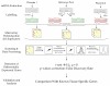
The general process in microarray experiments is depicted in figure 1. Fluorescent dyes are used to label the extracted mRNAs or amplified cDNAs from the tissue or cell samples to be analyzed. The DNA array is then hybridized with the labeled sample(s) by incubating usually overnight and then washing to remove non-specific hybrids. A laser excites the attached fluorescent dyes to produce light which is detected by a (confocal) scanner. The scanner generates a digital image from the excited microarray. The digital image is further processed by specialized software to transform the image of each spot to a numerical reading. This process is performed, first, finding the specific location and shape of each spot, followed by the integration (summation) of intensities inside the defined spot, and finally estimating the surrounding background noise. Background noise is generally subtracted from the integrated signal. This final reading is an integer value assumed to be proportional to the concentration of the target sequence in the sample to which the probe in the spot is directed to. In competitive two-dye assays, the reading is transformed to a ratio equal to the relative abundance of the target sequence (labeled with one type of fluorochrome) from a sample respect to a reference sample (labeled with another type of fluorochrome). In the one-dye Affymetrix technologies, the fluorescence is commonly yellow whereas in two-dyes technologies the colors used are green for reference and red for sample (although a replicate using dye-swap is common). The choice of the technology that is more appropriate depends on experimental design, availability, costs, and the expected number of expression changes. In general, when only a minority of the genes is expected to change, a two-dye or reference design is more suitable, otherwise a one-dye technology may be more appropriate.

Figure 1. Schematic representation of a gene expression microarray assay.

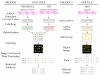
Arrows represent process (left column) and pictures or text represent the product. Differences in the protocol in one- and two-dye technologies are specific to the technology rather than samples or question. For CGH the process is similar replacing mRNA by gDNA.

Finally, at the end of the experiment an important issue derived from statistical tests in microarray data is the concept of the real significance of results and the concomitant need for multiplicity of tests. For example, when applying a t-test, the result is the probability that the observed values are given by chance. Commonly, we call a result significant when the probability is smaller than 5%. For large-scale data, a t-test would be performed thousands of times (one for each gene) which means that from 10,000 t-tests at 5% of significance level, we will call 500 genes differentially expressed merely by chance which is very close or even higher than those actually selected from experiments. Therefore, a correction to attempt to control for false positives should be performed. The most common correction method is the False Discovery Rate proposed originally by Benjamini and Hochberg (18) and extended by Storey and Tibshirani (19).

3. Applications in biomedical research

The ultimate output from any microarray assay, independently of the technology, is to provide a measure for each gene or probe of the relative abundance of the complementary target in the examined sample. In this section we revise the most common applications of the data derived from clinical studies using microarrays irrespective of the technology employed.

a. Relating Gene Expression to Physiology: Differential Expressed Genes

The most common and basic question in DNA microarray experiments is whether genes appear to be down-regulated (in which the expression has decreased) or up-regulated (in which the expression has increased) between two or more groups of samples. This type of analysis is essential because it provides the simplest characterization of the specific molecular differences that are associated to a specific biological effect. These signatures can be used to generate new hypothesis and guide the design of further experiments. A statistical test is used to assess each gene whether the expression is statistically different between two or more groups of samples (figure 2). When comparing population of individuals, a large number of samples per class are needed to avoid interference from variation due to individuals rather than experimental group. For laboratory controlled samples, such as cell-lines or strains, at least three biological replicates are recommended to compute a good estimate of the variance, hence the statistical confidence (as more replicates, as more confidence and less false positives). Using a statistical technique called power analysis it is possible to estimate the number of samples required to identifying a high percentage of truly differentially regulated genes. Although the use of this approach is common practice in the design of biological experiments it is still not widely spread in the microarray community.

Figure 2. Detection of Differential Expressed Genes.

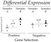
Large differences in gene expression are likely to be genuine differences between two groups of samples (A and B) whereas small differences are unlikely to be truly differences. Samples can be biological replicates or unreplicated populational samples.

To detect differential expressed genes, intuitive and formal statistical approaches have been proposed. The most famous intuitive approach, proposed in early microarray studies, is the fold change in fluorescence intensity (20, 21) expressed as the logarithm (base 2 or log₂) of the sample divided by the reference (ratios). In this way, fold change equal to 1 means that the expression level has increased two-fold (up-regulation), fold change equal to −1 means that the expression level has decreased two-fold (down-regulation) whereas 0 means that the expression level has not changed. Larger values account for larger fold changes. Genes whose fold change is larger that certain (arbitrary) value, are selected for further analyses. Although fold change is a very useful measure, the weaknesses of this criterion are the overestimation for low expressed genes in the reference (denominators close to zero tends to elevate the value of the ratio), the value that determines a “significant” change is subjective, and the tendency to omit small but significant changes in gene expression levels. For these reasons, nowadays the most sensible option is following formal statistical approaches to select differentially expressed genes. For two groups of samples the common t-test is the easiest option, whilst not the best, for analyzing two-dyes microarrays whose log₂ ratios generates normal-like distributions after normalization (see next section), and the ANOVA (analysis of variance) test for more than two groups of samples. These options apply for both one- and two-dye microarrays. If the data is non standardized, Wilcoxon or Mann-Whitney tests may be applied. A comparison of differential expression statistical tests, including t-test, has been published elsewhere (22).

The approaches we have described are univariate. That is, one gene is tested at the time independently of any other gene. There are multivariate procedures however, where genes are tested in combinations rather than isolated. Whilst being more powerful (23–26), these approaches require a more complex analysis.

b. Biomarker Detection: Supervised Classification

Disease type and severity are often determined by expert physicians or pathologists on the basis of patient symptoms or by analyzing features of the diseased tissue obtained by biopsy inspection. This categorization may allow the choice of appropriate pharmacological or surgical therapy. In this context, the availability of molecular markers associated to clinical outcome have been useful in allowing monitoring disease onset at a very early stage and complementing the clinical and histo-pathological analysis. The more recent application of DNA microarrays in clinical research has been a very important step towards the development of more complex markers based on multi-gene signatures. The identification of gene expression “signatures” associated to diseases categories is called biomarker detection or supervised classification (figure 3).

Figure 3. Biomaker Detection.

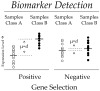
Larger differences in gene expression are more likely to be genuine differences between two groups of samples (A and B) than small differences. In this case, a large number of samples are more informative than individual replications.

The fundamental difference between identifying differentially expressed genes and identifying a set of genes of real diagnostic or prognostic value is that a biomarker needs to be predictive of disease class or clinical outcome. For this reason it must be possible to associate, to a given set of marker genes, a rule that allow deciding the identity of an unknown sample. The classification accuracy of the biomarker should also need to be determined with robust statistical procedures. Therefore, during the biomarker selection procedure, a substantial fraction of the samples are set aside to evaluate independently the accuracy of the selected biomarkers (in terms of sensitivity and specificity). Thus, such studies require a relatively large number of samples.

We already explained that unlike differential expression, in biomarker selection for diagnostics, a rule is needed to make predictions. This rule is generated by a classifier, a statistical model that assigns a sample to a certain category based on gene expression values. For example, a sensible classifier for diabetes is whether sugar levels in serum reach certain value. In statistics, this classifier is referred as univariate. That is, only one variable (sugar level) is needed in the rule. Nevertheless, for DNA microarray studies, it is common to obtain a large gene list useful for disease discrimination. Multiple genes provide robustness in the estimation and consider potential synergy between genes. Therefore, multivariate classifiers are commonly used. For example, it is well known that obesity and parental predisposition to diabetes, in addition to sugar levels in serum, is a more precise diabetes diagnosis criteria. Multivariate classifier can be designed using genes selected either by a univariate method such as t-test, ANOVA, Wilcoxon, PAM (27), Golub’s centroid (1), or by a multivariate method (23–26).

Thus, the possibility to characterize the molecular state of diseased tissues has lead to an improvement of prognosis and diagnosis as well as providing evidence of the existence of distinct disease sub-classes in previously considered homogeneous diseases.

c. Describing the Relationship between the Molecular State of Biological Samples: Unsupervised Classification

One key issue in the analysis of microarray data is finding genes with a similar expression profile across a number of samples. Co-expressed genes have the potential to be regulated by same transcriptional factors or to have similar functions (for example belonging to the same metabolic or signaling pathways). The detection of co-expressed genes may therefore reveal potential clinical targets, genes with similar biological functions, or expose novel biological connections between genes. On the other hand, we may want to describe the degree of similarity of biological samples at the transcriptional level (28). We may expect such analysis to confirm that samples with similar biological properties (for example samples derived from patients affected by the same disease) tend to have a similar molecular profile. Although this is true it has also been demonstrated that the molecular profile of samples is also reflecting disease heterogeneity and therefore it is useful in discovering novel diseases sub-classes (5). From the methodological prospective, these questions can be addressed using unsupervised clustering methods.

In this context, hierarchical clustering is, among several options (29), one of the most used unsupervised classification methods (figure 4). Other methods are available in several software packages such as R (http://cran.r-project.org), GEPAS (30), TIGR T4 (31), (32), GeneSpring (33) and Genesis (34). The core concept behind hierarchical clustering is the progressive construction of gene or sample cluster by adding one element (gene, sample, or a smaller cluster) at the time. In this way, more similar elements are added early to small clusters whereas less similar elements are added lately forming larger clusters. In order to decide which element is more similar to another, it is important to rely on a similarity or dissimilarity measure. Commonly used measures include Euclidean distance (defined as the geometrical distance between two elements in an n-dimensional space) and correlation distance. The result of the hierarchical clustering is therefore a hierarchical organization of patterns, similar to a phylogenetic tree. For example, in figure 4B the most similar genes 5 and 6 are first merged to form a cluster, then genes 1 and 2 form a different cluster which is lengthened later on by adding the next more similar gene 3; and the process continues until all genes have been included in a cluster and all clusters have been merged. For large-scale microarray data, it is common to use a simultaneous hierarchical clustering for samples and genes (32). Typically, genes are represented in the y-axis whereas samples are drawn in the x-axis..A color-coded matrix (heatmap), where samples and genes are sorted according to the results of the clustering, is used to represent the expression values for each gene in each sample. This two-dimensional clustering procedure is particularly suitable to explore the results of a large microarray experiment (figure 4).

Figure 4. Unsupervised classification and detection of co-expressed genes.

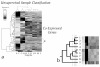
(A) Double-Hierarchical clustering of gene expression values (heatmap), in rows by genes, and in columns by samples. Similar samples (columns) generate clusters easily identified. For example, the gene expression of samples A and C is similar across genes. However A and C are different from the rest. Co-expressed genes (rows) form tight and small clusters. A selected cluster framed by dotted lines is shown in B. (B) Hierarchical generation of clusters from a selected group of genes in A.

d. Identification of Prognostic Genes Associated to Risk and Survival

In medicine, the association of prognostic factors related to survival times is invaluable. The link between gene expression levels and survival times may provide a useful tool for early diagnosis, prompt therapeutic, intervention, and in designing patient-specific treatments. Consequently, the selection of biomarkers that correlates with survival times is a very important objective in the analysis of microarray data. To date, a number of approaches have been developed. The most commonly used procedures incorporate genes into exponential, poison, or cox regression models using a univariate variable selection procedure (testing one gene at a time independently of any other; then, the most significant genes are selected as risk factors) (35). The gene selection procedure is summarized in figure 5. The selected genes combined with clinical classes can then be used to detect variations in survival times using both the Kaplan-Meier method and statistical tests. Often researchers are interested in finding subgroups of samples (independently of the recorded clinical data) whose survival times are significantly different. This information can then be used to prescribe specific treatments. In previous sections we have shown how unsupervised data exploration methods (such as cluster analysis) can be used to identify sub-groups of samples within a previously considered homogeneous disease. Once these sub-groups have been identified, survival analysis can be used to test whether they are characterized by different clinical outcomes (35).

Figure 5. Selection procedure for genes associated to survival times as risk factors.

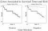
A positive gene (left plot) is that whose expression included as a risk factor in a survival model (cox, exponential, poison, etc.) can be fitted reasonably well (dotted line) to the original survival times (steep solid line). The predicted survival curve from a negative gene (dotted line in right plot) is not close to the observed survival curve (steep solid line).

e. Association of Genes to disease surrogate markers: Regression Analysis

An interesting question in the analysis of microarray data derived from clinical studies is whether there is an association between gene expression and an ordinal variable that represent a response, or more generally, a measure of disease progression (a surrogate marker). Examples of these variables are the concentration of metabolites, proteins in serum, response to treatment or dosage, growth, or any other clinical measure whose numerical representation makes sense progressively. The approach, depicted in figure 6, is conceptually similar to that introduced in the Survival analysis section of this review. The mathematical model in these case that relates the independent variable (such as time, levels of metabolites, protein, treatment) to dependent variables (genes) is, commonly, a linear regression model. Nevertheless, such model can be modified to include other available information.

Figure 6. Selection procedure for genes associated to outcome.

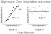
The expression of a positive gene (horizontal axis in left plot) is highly correlated with the associated outcome (vertical axis). For a non-associated gene (right plot), the gene expression (horizontal axis) is not correlated to outcome (vertical axis).

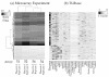
f. Genetic Disorders: Gene Copy Number and Comparative Genomic Hybridization

It is well known that several inherited diseases are a consequence of genetic rearragements such as gene duplications, translocations, and deletions. Moreover, these alterations are as well observed in cancer cells. A specific microarray technique used to detect these abnormalities in a single hybridization experiment is called Comparative Genomic Hybridization (CGH) (Pollack, 1999). The core concept in CGH is the use of genomic DNA (gDNA) in the hybridization to compare the gDNA from a disease sample versus that of a healthy individual. Hence, a typical microarray design can be used in this approach (figure 1). The signal intensity in all probes in the microarray should be therefore very similar for healthy samples. Thus, differences in gene copy number are easily detected by changes in signal intensity. Using this technology, Zhao et al., (2005) have recently characterized the variations of gene copy number in several cell lines derived from prostate cancer and Braude et al., (36) confirmed an alteration in chronic myeloid leukaemia.

g. Genetic Disorders: Epigenetics and Methylation

Around 80% of CpG-dinucleotides are naturally methylated at the fifth position of the cytosine pyrimidine ring (37). The patterns of cytosine methylation along with histone acetylation and phosphorylation controls the activation and deactivation of genes without changing the nucleotide sequence (38). These regulatory mechanisms are known as the epigenetic phenomena. In particular, genes methylated in their promoters become inactive irrespective of the presence of the transcriptional activators. Aberrations in any of these epigenetic patterns cause several syndromes and may predispose carriers to cancer (39). To detect patterns of methylation using microarrays, two main methods have been proposed (40). One is based in the enrichment of the unmethylated fraction of CpG islands and the other focuses on the hypermethylated fraction. Both methods make use of methylation sensitive restriction enzymes to generate fragments enriched in either, unmethylated or methylated CpG sites (figure 7). In the first method, sample and control gDNA are cleaved with methylation-sensitive enzymes that cut unmethylated CpG sites generating protruding shorter fragments leaving methylated CpG sites unaltered. Specific adaptors are then linked to these protruding ends. Methylated fragments are subsequently cut by a CpG specific enzyme. The remaining fragments that contain the adaptor, those that were originally unmethylated, are amplified by PCR using and primers complementary to the adaptors sequence. The result is that genes belonging to the unmethylated fraction are associated to higher fluorescent intensities on the microarray. On the other hand, in the second method, the gDNA from sample and control samples are cleaved with a restriction enzyme to generate small protruding fragments. Fragments are then linked to adaptors and cut by methylation sensitive restriction enzymes leaving methylated flanked fragments unaltered which are amplified using PCR. The result is that the methylated fraction is amplified and detected in the microarray. The microarrays used in these experiments are therefore specially designed to include such fragments. Using the methods described, methylation patterns have been screened for several types of cancers (41–46).

Figure 7. Detection of altered methylated patterns and DNA polymorphisms in genomic DNA.

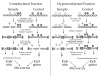
Left Panel: Enrichment of unmethylated DNA fragments (see text). Right Panel: Enrichment of hypermethylated fragments (see text). Scheme adapted from Schumacher et al. (2006).

h. Genetic Disorders and Variability: Gene Polymorphism and Single Nucleotide Polymorphism

The human genome carries at least 10 million nucleotide positions that vary in at least 1 of 100 individuals in a population (47). The identification of these single nucleotide polymorphisms (SNPs) is an important tool for identifying genetic loci linked to complex disorders (47). Although there are commercially available microarrays to detect SNP, these technologies are still in their infancy and the widespread distribution is still halt because of the relatively high cost per sample. So far, the number of SNPs stored in public databases is more than 2 millions whereas the available microarrays for SNPs detection only cover 10,000 SNPs. The three major strategies for SNP genotyping using microarrays are all based on primer extension techniques depicted in figure 8. The primer included in the microarray probe hybridizes to the target sequence precisely adjacent to its SNP. The first strategy (figure 8a) consists of mini-sequencing the primer specific for each polymorphism immobilized in the microarray support. PCR products, DNA polymerase, and different color fluorescent labeled nucleotides are added in the hybridization-one-base-extension to detect the SNPs in parallel. The genotype is detected by color combinations. The second strategy (figure 8b) uses the same concept of primer specific hybridization, though combined with only one dye and more than one base extension. The genotype is revealed by signal strength. The third strategy (figure 8c) makes one-base extension in solution combined with different color fluorescent-labeled nucleotides. Primers are then captured by hybridization in the microarray. The genotype is detected by color combinations. Recent studies have produced genome-wide SNP characterization for a number of tumor types (48–50).

Figure 8. Major techniques for detection of SNPs using microarrays.

Colors and patterns are used for illustrative purposes. Scheme adapted from Syvanen (2005).

i. Chromatin Immunoprecipitation: Genetic Control and Transcriptional Regulation

Transcription factors (TF) are regulatory proteins that can bind specific DNA sequences (usually promoters) to control the level of gene expression. Mutations or alterations in the expression or activation of TF are known in several diseases (51). For example, abnormal over-expression of the TF c-Myc is found in 90% of gynaecological cancers, 80% of breast cancers, 70% of colon cancers, and 50% of hepatocarcinomas (52). Therefore establishing the link between TF and their targets is essential to characterize and design better cancer therapies. To identify these targets, DNA fragments are incubated with a selected TF that has been tagged (figure 9). The complex DNA-TF is precipitated using a quite specific antibody against the tagged peptide. Precipitated DNA is then labeled and hybridized in DNA microarrays to reveal genome-wide targets for the selected TF (figure 9). An experimental overview and computational methods for the analysis of these data have been revised elsewhere (53, 54).

Figure 9. Chromatin immune-precipitation (ChIP-on-chip) assay.

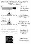
The generation of a hybrid gene between a gene for a transcription factor (TF) and a tag coding sequence renders a quimaeric TF. Upon binding to its DNA target the complex can be pulled-down from the tag to recover such type of DNA sequences.

j. Pathogen detection

Classically, pathogen detection is achieved through a series of clinical tests which detect, generally, single pathogens. A battery of clinical assays is therefore performed to typify a sample. A radical recent approach uses DNA microarrays to test for the presence of hundreds of pathogens in a single experiment (15, 16). For this, known sequences from each pathogen are collected and those being pathogen-specific are selected (figure 10). The collection of specific sequences is used to build a purpose-specific microarray. Then genomic DNA from a patient biopsy or from a food sample suspected to be infected is extracted and hybridized to the microarray. Pathogen detection is simply revealed by spot intensity.

Figure 10. Multi-pathogen detection using DNA microarrays.

Specific DNA sequences from disease-causing micro-organisms can be spotted on a microarray for pathoghen detection.

4. An Overview of a Typical Microarray Experiment

In this section we provide a brief description of the typical workflow of a microarray experiment and its data analysis (see figure 1).

RNA Extraction

RNA can be extracted from tissue or cultured cells using molecular biology laboratory procedures (although several commercial kits are available). The amount of mRNA required is about 0.5μg which is equivalent to 20μg of total RNA, though there is some variation depending on the microarray technology. When the amount of mRNA (or DNA) is scarce, an amplification step, for example by PCR amplification of reverse transcribed cDNA, is needed before labeling.

Labeling

mRNA is retro-transcribed using reverse transcriptase to generate cDNA. Labeling is achieved by including in the reaction (or in a separate reaction) modified fluorescent nucleotides that are made fluorescent by excitation at appropriate wavelengths. The most common fluorescent dyes used are Cy3 (green) and Cy5 (red). The unincorporated dyes are usually removed by column chromatography or ethanol precipitation.

Hybridization

Hybridization is carried out according to conventional protocols. Hybridization solution contains saline sodium citrate (SSC), sodium dodecyl sulphate (SDS) as detergent, non-specific DNA such as yeast DNA, salmon sperm DNA, or repetitive sequences, blocking reagents like bovine serum albumin (BSA) or Denhardt’s reagent, and labeled cDNA from the samples. Hybridization temperatures range from 42°C to 45°C for cDNA-based microarrays and from 42°C to 50°C for oligo-based microarrays. Hybridization volumes vary between 20μl to one ml depending on the microarray technology. A hybridization chamber is usually needed to keep temperature and humidity constant.

Scanning

After hybridization, the microarray is washed in salt buffers of decreasing concentration and dried by slide centrifugation or by blowing air after immersion in alcohol. The slide is then read by a scanner which consists of a device similar to a fluorescence microscope coupled with a laser, robotics, and digital camera to record the fluorescent excitation. The robotics focuses on the slide, lens, camera, and laser by rows similar to a common desktop scanner. The amount of signal (color) detected is presumed to be proportional to the amount of dye at each spot in the microarray and hence proportional to the RNA concentration of the complementary sequence in the sample. The output is, for each fluorescent dye, a monochromatic (non-colored) digital image file typically in TIFF format. False-color images (red, green and yellow) are reconstructed by specialized software for visualization purposes only.

Image Analysis

The goal in this step is to identify the spots in the microarray image, quantify the signal, and record the quality of each spot. Depending on the software used, this step may need some degree of human intervention. The digital images are loaded in specialized software with a pre-loaded design of the microarray (grid layout) which instructs the software to consider number, position, shape, and dimension of each spot. The grid is then accommodated to the actual image automatically or manually. Fine-tuning of spot positions and shapes is usually performed to avoid any bias in the robotic construction of the microarray. Human involvement is needed to mark those spots that could be artifacts such as bubbles or scratches which are common. Finally, an automated integration function is performed using the software to convert the actual spot readings to a numerical value. The integration function considers the signal and background noise for each spot. The output of the image analysis may be commonly a tab-delimited text file or a specific file format. Common image analysis software include ScanArray® (PerkinElmer), GenePix® (Axon), TIGR-SpotFinder/TM4 (www.tigr.org), and GeneChip® (Affymetrix) This process varies, from automatic or semi-automatic to manual, depending on the microarray technology, scanner and software used.

Normalization

Systematic errors are introduced in labeling, hybridization and scanning procedures. The main aims of normalization is to correct for these errors preserving the biological information and to generate values that can be compared between experiments, especially when they were generated in, and with, different times, places, reagents, microarrays, or technicians. There are two types of normalization, within and between array normalization. Within array normalization refers to normalization applied in the same slide and it is applicable, generally, to two-dye technologies. For this, let us define M=Log₂(R/G) and A=Log₂(R*G)/2 where R and G are the red and green readings respectively. Under the assumption that the majority of genes have not been differentially expressed, the majority of the M values should oscillate around zero. Within normalization is finally performed shifting the imaginary line produced by the values of M (in vertical axis) to zero along the values of A (in horizontal axis). This kind of normalization, sometimes called loess, is usually performed by spatial blocks to avoid any bias in the microarray printing process (called print-tip-loess). Between normalization is necessary when at least two slides are analyzed to guarantee that both slides are measured in the same scale and that its values are independent from the parameters used to generate the measurements. The goal is to transform the data in such a way that all microarrays have the same distribution of values. For two-dye technologies this is optional and is commonly done through scaling or standardizing the values once within normalization has been performed. For one-dye microarrays, between normalization is usually performed using methods to equalize distributions such as quantile-normalization (55) after log₂ transformation. There are, however, a number of normalization methods. The right choice is usually data-dependent. A comparison of the results of different normalization methods is recommended.

Missing Values

The image analysis process (generally in spotted microarrays) does not always generate a value for a gene because the spot was defective or manually marked as faulty. This is not a major issue when genes are replicated in several spots in the microarray, because the reading of the gene can still be estimated using the remaining spots. If the value in a spot is systematically missing in several arrays, it should be removed from the analysis. If the number of missing values is low, the corresponding spots can be simply not considered in all arrays. However, when the number of arrays is large this could lead to the removal of several spots. To avoid these problems, one must use only those methods that can deal with missing values, or, use algorithms to infer those values (30). Results should, therefore, be interpreted considering that some values were inferred.

Filtering

Current microarrays contain more than 10,000 genes, spots, or probes. Dealing with large amount of data may require expensive computational resources and large processing times. A common practice is to remove genes that have not shown significant changes across samples, genes with several missing data, or those whose average expression is very low (because low expressed genes are more susceptible to noise). The most common approaches use statistical tests (lower), signal to noise estimations (higher), variability (higher), and average (higher).

Transformation

The numerical values from image analysis are commonly integer numbers between 1 and 32,000 for both signal and background. The background is normally subtracted from the signal. The distribution of these values is however concentrated in a narrow range and is therefore transformed using logarithms (base 2 generally) which generates normal-like distributions. Negative values resulting from subtraction may raise problems in transformations which are resolved by restricting the values or performing more robust transformations such as the generalized logarithm.

Statistical Analysis

The procedure after image analysis and data processing depends mainly on the particular biological issue and data available. These procedures have been described in the section 3 (Applications).

5. Illustrating the detection of differentially expressed genes: the case of term placenta

In previous sections we have introduced the experimental and data analysis methods used in common microarray experiments. In order to illustrate these procedures we will use a case study designed to identify genes that are preferentially expressed in placenta. This study, currently ongoing in our laboratory, is part of a larger project whose results are expected to assist further research revealing molecular mechanisms involved in fetus development, placental function, and pathologies related to pregnancy. In order to identify genes specific for human placenta, we used a two-color microarrays. In this experiment, mRNA extracted from two normal human placentas was compared with a pool of mRNA extracted from several normal tissues not including placenta. In order to gain information on the variability expected from experimental errors, we also compared two aliquots of the reference mRNA in the same array. An overview of the process is depicted in figure 11. A brief description of the detailed procedure follows.

Figure 11. Experimental design of the placenta microarray experiment.

RNAs from two term human placentas were compared to RNAs from a collection of human tissues, except placenta, in search of placental specific transcripts.

Step 1: mRNA extraction and Microarray Hybridization

Human total term placenta RNA (isolated using proteinase K-phenol based protocol as described in (56)) and a pool of total RNAs from several human tissues not including placenta (commercially available) were part of the set of reagents utilized in the EMBO-INER Advanced Practical Course 2005 (http://www.embo.org/courses_workshops/mexico.html and http://chipskipper.emblde/iner-embo-course/index.htm). They were quality controlled by running them in a RNA 6000 Nano Assay from Agilent. First strand cDNA was synthesized from each RNA (5 μg) sample by reverse transcription using an oligo-dT primer with a TT-promoter sequence attached to its 5′ end, while second strand resulted from treating the first strands with RNase H plus DNA polymerase I (Message Amp aRNA kit from Ambion). Column purified double-stranded cDNAs were transcribed (in vitro transcription) with T7 RNA polymerase and the amplified RNAs (aRNAs) were purified also by column binding and subsequent elution. Fluorescent labels were indirectly attached to the hybridization probes by a two-step procedure. The first step consisted of a reverse transcription of the aRNA using this time a mixture of all four desoxiribonucleotides and including aminoallyl-dUTP. In the second step, N-hydroxysuccinimide-activated fluorescent dyes (Cy3 and Cy5) were coupled to the cDNAs by reaction with the amino functional groups. Probes were preincubated with blocking reagents (human Cot DNA at 1 μg/ml and poly-dA DNA also at μg/ml) and then hybridized to prehybridized (6X SSC, 0.5% SDS and 1% BSA) slides in hybridization buffer (50% formamide, 6X SCC, 0.5% SDS and 5X Denhardt’s solution). Slides were washed (once in 2X SSC/0.1% SDS at 65°C for 5 minutes, twice in 0.1X SSC/0.1% SDS but first at 65°C for 10 minutes and then at room temperature for 2 minutes, and finally in isopropanol also at room temperature, with slide centrifugation between each washing step) and stored in the dark until scanning. Fluorescent probes were hybridized to cDNA microarrays (laboratory made oligo-based microarray containing half of the probes in each of two slides).

Step 2: Microarray Scanning, Spot Finding and Image Processing

Microarrays were scanned using (ScanArray Express, PerkinElmer). Images obtained were analyzed using ChipSkipper ® (http://www.embl-em.de) to obtain a single value for each spot representing the ratio (in log₂ scale) of the mRNA expression level from placenta to the reference mRNA from the pool of non-placenta tissues. A value of 0 represents similar expression level in both mRNA samples. A value of 1 represents twofold over-expression in placenta whereas a value of −1 represents two-fold down-regulation in placenta. One placental sample was hybridized in duplicate into the two microarrays using a dye-swap design. In this approach the labeling scheme is reversed in two separate microarrays. To gain information on the variability associated to experimental error, two aliquots of the reference pool mRNA were compared on the same microarray. Likewise the comparison between experimental and control samples, the comparison between the two control samples was performed in duplicate using the dye-swap design. To summarize, the experiment was performed using six microarrays (two placentas samples compared with a reference in duplicate and two reference mRNA as controls, see figure 11).

Step 3: Quality Assessment, Processing and Normalization

To ensure that all microarrays were comparable in scale, we performed print-tip loess normalization (shifting the imaginary M line to zero, see figure 12). We processed the dataset removing from the analysis all control and empty spots. Representative plots before and after within normalization and processing for both placenta and control experiments are shown in figure 12. Note that, as expected, there are important differences in ratio values (M value in figure 12c–d) for highly expressed genes (A value) in placenta compared with the reference (figure 12c), whereas ratios in the control experiment are very close to zero (figure 12d) indicating a very high reproducibility of the technology.

Figure 12. Quality Assesment and Normalization.

(a) Ratio values (M=Log2(R/G), R=Red channel, G=Green channel) versus average values (A=Log2(R*G)/2) for one placenta sample. Dots represent spots in the microarray. Crosses correspond to control spots. Lines represent the tendency for each block (print-tip) in the microarray. (b) Control assay, two reference mRNA aliquots were hybridized changing the dye color only. Symbols like in (a), (c) Normalized data from (a), (d) Normalized data from (b). Control spots removed in (c) and (d).

Step 4: Detection of Differential Expressed Genes

Duplicated spots were averaged to generate a unique measure per gene per array. To detect differential expressed genes we used a one-sample t-test under the null hypothesis of no differential expression (mean ratio equal zero). Resulted p-values were adjusted for multiplicity tests using the False Discovery Rate (FDR) approach (18, 57). Because of the small number of samples, we treated the replicated biological samples as independent* to increase the level of confidence in the statistical tests, and we limited the selection of differentially expressed genes to those that fulfill two conditions: firstly, genes whose FDR value is less than 0.10 (10% corresponding to raw p-values less than 0.0000118), and secondly, genes whose absolute fold expression is at least two. Using these criteria, 350 (out of 21,456) were selected. A subset of 205 genes is depicted in figure 13 (see step 5).

Figure 13. Genes differentially expressed in placenta compared to other tissues.

(a) Heatmap showing the relative gene expression in placenta. Darker color means higher expression in placenta. Genes are ordered using a hierarchical clustering algorithm, (b) Heatmap showing the score in T1dbase corresponding to genes in (a). Darker colors represents more specific expression.

Step 5: Validation

In order to verify the process of selection, we made two comparisons. First, as negative control, we followed the same selection criteria for the control microarrays that made use of the reference sample in both channels. The result was that no genes match the criteria. Second, we performed a comparison using T1dbase (http://www.t1dbase.org/page/TissueHome) from Tissue Specific Expression Tool (58). This tool makes use of Gene Expression Atlas (59), SAGEmap (60), and TissueInfo (58), integrating all measurements in a single score (58). This score, estimated for several tissues, represents whether the expression for a gene is tissue-specific. Scores closer to 1 are meant to be tissue-specific whereas scores closer to 0 represents no-tissue-specificity. From the 350 genes resulted in step 4, we selected only those that are also included in this database. The result was 201 genes. Several genes that seem to be over-expressed in the placentas processed here (darker colors in figure 13a) shows consistently higher placenta-specific scores in T1dbase (darker colors in figure 13b). These results suggest that the experiment is coherent and valid.

Step 6: Analysis

Once genes have been selected, further computational, literature and laboratory analyses are needed to confirm, expand, or restrain the results. Here, the analysis only dealt with comparing the results with T1dbase-Tissue Specific Expression Tool. However, queries to Gene Ontology, KEEG pathways, Pubmed, Blasts, or any other pertinent database resource should be considered a compulsory step.

6. Conclusions and Trends

DNA microarrays are a powerful, mature versatile and easy-to-use genomic tool that can be applied for biomedical and clinical research. The research community is expanding the use of this approach for novel applications. The main advantage is the genomic-wide information provided at reasonable costs. Biological interpretation however requires the integration of several sources of information. In this context, a new discipline referred as Systems Biology is emerging that integrates biological knowledge, clinical information, mathematical models, computer simulations, biological databases, imaging, and high-throughput “omic” technologies, such as microarray experiments. Therefore, multidisciplinary groups involving clinicians, biologists, statisticians, and recently bioinformaticians are being formed and expanded in all important research institutions. Subsequently, virtually all biology-related research areas are moving from merely describing cellular and molecular components in a qualitative manner, towards a more quantitative approach. These new teams are generating huge amounts of data and more convincing models to ultimately reveal hidden pieces in the biological puzzle. This new knowledge is having a crucial impact on the treatment of diseases, since among other things individualizes subtypes of pathologies, disease risks and survival, treatment prognosis and outcome, quickly approaching biomedical research to the era of personalized medicine.

APPENDIX

Microarray-Related Public Resources

To date, hundreds of microarray studies have been published in the literature. Researchers tend to make microarray data available through internet, generally in proprietary web-sites or public microarray database repositories (Table 1). These public repositories generally follow the minimum information about a microarray experiment (MIAME) compliance format (61) or microarray gene expression markup language (MAGE-ML) (62). As these repositories may contain unpublished data, it is important to consult these public repositories before embarking on a new microarray project. There are dozens of software tools for analyzing microarray data and still there is a tendency for publishing new software every day. A list of general common software is provided in Table 2. These tools are created by multidisciplinary groups across the world to solve particular problems. There is however several software “flavours”, that is, several tools to solve the same problem in a slightly different way (statistical model, data format, or user-interface). This generates the pitfall that software is isolated or not easy to connect with others in a pipeline. The result is that users commonly have a large collection of tools with many manual or complex steps to transfer information between them.

Table 1.

Common public microarray repositories

Database	URL
Gene Expression Omnibus (GEO)	http://www.ncb.nlm.nih.gov/geo
ArrayExpress	http://www.ebi.ac.uk/arrayexpress
Stanford Microarray Database (SMD)	http://genome-www5.stanford.edu
Another Microarray Database (AMAD)	http://www.microarrays.org/
Oncomine	http://www.oncomine.org

Table 2.

Common free software containing collections of tools

Software: Major Tools	URL
GEPAS:	http://www.gepas.org
Transformation, Normalization, Filtering, Missing Values Imputation, Differential Expression, Classification, Regression, Survival, Clustering, Visualization, Gene Ontology
T4 Suite (TIGR):	http://www.tigr.org/software/microarray.shtml
Image Analysis, Visualizations, Differential Expression, Principal Component Analysis, Clustering, Classification, other in plug-ins
SAM (Excel):
Differential Expression, Regression, Survival, Classification
Expression Profiler (EP:NG):	http://www.ebi.ac.uk/expressionprofiler
Tranformation, Normalization, Filtering, Missing Values Imputation, Differential Expression, Classification, Clustering, Visualization
Bioconductor (under R language/environment):	http://www.bioconductor.org
All tools, very robust, programmable, allow plug-ins, no friendly interface.
AMIADA:	http://dambe.bio.uottawa.ca/amiada.asp
Transformation, Principal Component Analysis, variety of cluster analysis, other graphic functions
caGEDA:	http://bioinformatics.upmc.edu/GE2/GEDA.html
Transformation, Normalization, Differential Expression, Classification
GenePattern:	http://www.broad.mit.edu/cancer/software/genepattern/
Transformation, Normalization, Filtering, Missing Values Imputation, Differential Expression, Classification, Regression, Survival, Clustering, Visualization, Gene Ontology, programmable pipeline, allow plug-ins.
Genesis:	http://genome.tugraz.at/Software/Genesis/Description.html
Filtering, Missing Values, Normalization, Clustering, Principal Component Analysis, Visualization, Differential Expressed Genes, Classification, Gene Ontology,