Recombination rate estimation in the presence of hotspots

Abstract

Fine-scale estimation of recombination rates remains a challenging problem. Experimental techniques can provide accurate estimates at fine scales but are technically challenging and cannot be applied on a genome-wide scale. An alternative source of information comes from patterns of genetic variation. Several statistical methods have been developed to estimate recombination rates from randomly sampled chromosomes. However, most such methods either make poor assumptions about recombination rate variation, or simply assume that there is no rate variation. Since the discovery of recombination hotspots, it is clear that recombination rates can vary over many orders of magnitude at the fine scale. We present a method for the estimation of recombination rates in the presence of recombination hotspots. We demonstrate that the method is able to detect and accurately quantify recombination rate heterogeneity, and is a substantial improvement over a commonly used method. We then use the method to reanalyze genetic variation data from the HLA and MS32 regions of the human genome and demonstrate that the method is able to provide accurate rate estimates and simultaneously detect hotspots.

Direct measurement of recombination rates is a technically difficult process. Even large-scale pedigree studies produce low-resolution rate estimates because of the relatively low number of meioses that can practically be observed (Kong et al. 2002). An alternative technique of sperm typing, which allows for many thousands of meiotic products to be screened from a single individual, produces extremely high-resolution estimates. However, these studies are male-specific, are typically only applied to a few individuals and are currently limited in scale to only small (<1 Mb) regions of the genome (Arnheim et al. 2003; Jeffreys et al. 2004; Greenawalt et al. 2006).

Despite the technical challenges, such experimental techniques have shown that the spatial location of recombination events in humans is nonrandom (Kauppi et al. 2004). It has become clear that meiotic recombination events tend to occur in highly localized regions (<5 kb) on the chromosome known as recombination hotspots, and the peak recombination rate within these hotspots can be hundreds of times that of the surrounding region (Jeffreys et al. 2005).

Statistical analysis of population genetic data provides an alternative means of recombination rate estimation. A number of methods have been proposed for estimating the population genetic recombination rate (Wall 2000; Fearnhead and Donnelly 2001; Li and Stephens 2003; McVean et al. 2004; Smith and Fearnhead 2005). However, the most available methods either assume a constant recombination rate across the region or cannot be applied on a genome-wide scale.

In an attempt to address these issues, a statistical method was previously developed that aims to perform inference on the fine-scale structure of recombination rate variation from genome-scale data (McVean et al. 2004). This method, distributed in the LDhat package (specifically, the interval program), uses a Bayesian reversible-jump Markov chain Monte Carlo (rjMCMC) scheme to fit a piecewise-constant model of recombination rate variation. However, rather than calculating the full coalescent likelihood, a composite-likelihood approximation is employed (Hudson 2001). Simulations have shown that the LDhat produces largely unbiased rate estimates of the fine-scale genetic map. A further advantage of LDhat over similar population-based methods is that it is currently one of only a few available statistical methods that can be applied to samples containing up to ∼200 chromosomes at a genome-wide scale. The application of this method to large data sets has established that hotspots are apparently a ubiquitous feature of the human genome with between 25,000 and 50,000 expected to exist (McVean et al. 2004; Myers et al. 2005) and has started to reveal the relationship between recombination and other genome features (Myers et al. 2006; Spencer et al. 2006).

However, no model of recombination hotspots was included in LDhat, and hence the true level of heterogeneity implied by the presence of recombination hotspots may be poorly captured. In this paper, we describe an extension to the LDhat rate estimation scheme that includes a description of recombination hotspots. By incorporating a hotspot model, it is expected that the accuracy of rate estimates can be improved. Furthermore, the method can simultaneously estimate the properties of recombination hotspots as part of the rate estimation procedure.

Methods

In this paper, the parameter of primary interest is the map of population-scaled recombination rate ρ = 4N_er, where N_e is the effective population size, and r is the map of the sex-averaged recombination rate (expressed in terms of expected cross-over events per generation per kilobase between adjacent SNPs). Given a sample of unrelated chromosomes from a population, we would like to make inferences about ρ. To do so, we need to calculate the likelihood of the data, which is proportional to P(D|ξ), where D is the data (the haplotypes or genotypes in our sample) and ξ represents our model parameters (i.e., ρ and the population mutation rate, θ). Calculating the full coalescent likelihood of the data is currently computationally prohibitive on all but the smallest of data sets (Fearnhead and Donnelly 2001). We therefore have adopted a method for calculating an approximation to the full likelihood, known as the composite likelihood, which we will now describe.

The composite likelihood scheme (Hudson 2001; McVean et al. 2002) considers only pairs of single nucleotide polymorphisms (SNPs) in the data. For each pair of SNPs, a coalescent model is used to calculate a likelihood surface over a range of recombination rates. A pseudo-likelihood is then constructed as the product of the likelihood over all pairs of SNPs in the region under consideration. Compared to full-likelihood approaches, the required computation is reduced by many orders of magnitude, making the composite scheme suitable for much larger data sets.

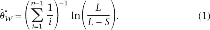
As the first stage of the composite scheme, a population mutation rate is estimated using an approximate finite-sites version of the Watterson estimate (Watterson 1975). Given n sampled gene sequences of length L, with S segregating sites, the population mutation rate per site is estimated using:

In the second stage, pairs of sites with only two alleles are grouped into equivalent sets. As an example, suppose we have five sequences. For one pair of SNPs, the haplotypes are AA, AT, TA, TA, and AA, which have the minor allele “T” at both sites. For a separate pair of SNPs, the haplotypes are GG, CC, CG, GG, and CG, which have the minor allele “G” at the first site and “C” at the second site. These sets are both equivalent to the unordered set (11, 10, 01, 01, 11), where 0 represents the minor allele at each site. The number of sets is dependent on the number of sequences and the variability in the data set. Assuming that every possible combination occurs in a data set, the number of uniquely identifiable sets scales with an order of n³.

The third stage is to estimate the likelihood of each set (i.e., each pair of SNPs). This is achieved using the importance sampling method of Fearnhead and Donnelly (2001). Informally, a large number of genealogies are generated for each set at the assumed mutation rate using a stochastic process (allowing for reverse mutation) and over a range of population-scaled genetic distances (a typical range would be 0 ≤ ρ ≤ 100). The likelihood at each genetic distance is calculated by averaging over the importance weights of the sampled genealogies. This method is not usually tractable for large data sets due to the large number of genealogies that need to be generated. However, by considering only pairs of SNPs, the method becomes practical for data sets containing hundreds of sequences and thousands of SNPs. In such a way, it is possible to precalculate and store likelihood tables for any data set of a given number of haplotypes.

Finally, given the precalculated likelihood surface, we can calculate a pseudolikelihood of the data using an assumed genetic map. To construct the pseudolikelihood, we assume that pairs of SNPs are independent of each other (although in reality they are not). In the original LDhat implementation, given a vector of recombination rates, ρ, in which the i^th element gives the population scaled recombination rate between the i^th and (i+1)^th SNP, the composite likelihood is given by:

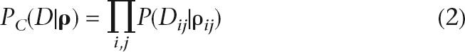where P(D_ij|ρ_ij) is the likelihood of the data at segregating sites i and j given a population-scaled genetic distance of ρ_ij between them (extracted from the map). This approximation to the true likelihood surface is required to keep the computational cost down. Nevertheless, the vast majority of the computational cost of the composite scheme is contained in the importance sampling section. Likelihood tables have been precalculated for a variety of possible data sets of up to 192 chromosomes and are available for download at http://www.stats.ox.ac.uk/~mcvean/LDhat.

A strong advantage of the composite scheme is the ability to use genotype data. As only pairs of SNPs are considered, genotype data can be considered by summing over all possible phases of each SNP pair. In a similar manner, the scheme can incorporate missing data although the efficiency of the algorithm does not scale well with increasing amounts of missing data. Loci with more than ∼10% missing data should generally be discarded.

Compared to full-likelihood methods, the likelihood surface of the composite scheme tends to be sharply peaked. However, the maximum-likelihood estimate of the two methods is well correlated (McVean et al. 2002). Unfortunately, the peaked nature of the composite scheme can be unsuitable for use with rjMCMC, as the chain may become stuck in a local maximum. In our case, we found that the original composite likelihood severely limited the mixing of our method. We have therefore informally investigated adaptations of the composite likelihood which would in some sense “flatten” the likelihood surface and hence allow the method to mix well. Given S SNPs, a suitable alternative to Equation 2 is given by:

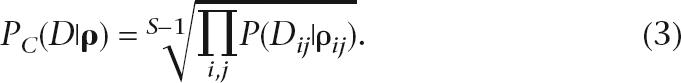Intuitively, the correction can be thought of as a correction for the inherent double counting in the composite likelihood. In the case of ρ = ∞, the original composite likelihood is equal to the (S − 1)^th power of the full likelihood, due to each SNP interval being considered multiple times. The (S − 1)^th root was therefore chosen as a suitable correction, although it will tend to over-flatten the likelihood for small recombination rates.

In order to maintain the computational feasibility of the method, we do not consider the contribution to the composite likelihood from SNPs separated by more than 50 intermediate SNPs. That is, we assume P(D_ij|ρ_ij) = 1 if |i − j| > 50 and adjust the root in Equation 3 accordingly. The choice 50 SNPs is arbitrary, but it was found that using larger subsets did not significantly improve the results (data not shown). Furthermore, there are both theoretical and empirical studies that suggest that limiting the number of SNPs may actually improve the performance of the estimator (Fearnhead 2003; Smith and Fearnhead 2005).

To obtain a pseudoposterior distribution on ρ, the original LDhat method imposed a prior of piecewise-constant structure with constant recombination rate over SNP intervals and change-points located only at SNPs. In the new scheme, we maintain a similar structure for the estimation of background recombination rates, with the exception that change-points are no longer restricted to SNP locations. The major novelty of the method comes from the incorporation of a hotspot model. We model hotspots as sharp peaks in the recombination rate with a double exponential shape. Under our prior model, hotspots are uniformly scattered along the analyzed region with the number of hotspots and their properties (such as position, heat, and width) determined as part of the rjMCMC scheme. To illustrate the differences between the LDhat prior and the new prior, we have generated individual realizations of each (Fig. 1). Full details of the prior and the reversible jump moves are contained in the Supplemental material (Appendices A and B).

Figure 1.

Illustration of the priors of LDhat (A) and rhomap (B). Shown here are individual realizations of the priors for a 200-kb region. Note the difference in the Y-axis scales.

Results

Simulation studies

We have implemented the new method in the program rhomap, which is incorporated into the LDhat package (version 2.1; available for download from http://www.stats.ox.ac.uk/~mcvean/LDhat/). In the following section, we use rhomap to refer to the new method and LDhat to refer to the original implementation. To investigate the performance of rhomap, we undertook four simulation studies. In the first study, we simulated data with a constant recombination rate. In the second, we simulated data with a randomly chosen variable recombination rate. In the third study, we simulated data using three fixed recombination maps. In the fourth study, we investigated the effect of thinning the SNPs in the data on the rhomap estimates. Each study simulated data sets containing 100 haplotypes 200 kb in length. Data was simulated using the fin program (McVean et al. 2002; http://www.stats.ox.ac.uk/~mcvean/LDhat/). The simulation population-scaled mutation rate per site was 3.86 × 10⁻⁴, giving an expected number of segregating sites of 400.

In all four simulation studies, rhomap was run for a total of 1,100,000 iterations which included a burn-in of 100,000 iterations. Samples of the chain were taken every 100 iterations after the burn-in. The block and hotspot penalties were set to zero (a note on choosing penalties can be found in the Supplemental material, Appendix D). For comparison, the data sets were also analyzed with the LDhat method using 10 million iterations and a block penalty of 5 (as used by Jeffreys et al. 2005; Myers et al. 2005). With the above parameters, the computational cost of the two methods is approximately equal. Using a 1.8-GHz personal computer, both methods take ∼17 min to analyze a typical data set from these simulation studies. However, rhomap scales less favorably with the number of SNPs than LDhat.

Simulation Study A

We simulated 100 data sets using a fixed recombination rate of ρ = 0.5/kb, giving a total recombination distance for the region of R = 100. In this study, rhomap tends to slightly overestimate the total map length, with LDhat estimates being less biased (Fig. 2A,B). The average estimates of ρ/kb are 0.58 for LDhat and 0.65 for rhomap (Fig. 3A). The upward bias in the rhomap estimates is caused by the weakness of the flattened composite likelihood relative to the prior, allowing the method to insert spurious hotspots. However, as will be seen in the next simulation study, the upward bias primarily affects estimates of background rate variation and is less of a problem in the presence of hotspots.

Figure 2.

Deviation of the estimated total ρ from the simulated value. Rate estimates from the constant rate simulations (Simulation Study A) using LDhat and rhomap are shown in A and B, respectively. Rate estimates from the variable rate simulations (Simulation Study B) using LDhat and rhomap are shown in C and D, respectively.

Figure 3.

Average recombination rate estimates from 100 simulated data sets. (A) Results from Simulation Study A with a constant recombination rate. (B) Results from Simulation Study C with an active central hotspot. Rate estimates from LDhat and rhomap are shown as thick red and blue lines, respectively. The simulated recombination profile is shown in black. The 2.5th and 97.5th percentiles of the estimated rates are shown in faded colors. Note that, for clarity, the constant rate simulation estimates are shown on a linear scale, whereas the hotspot simulation estimates are shown on a logarithmic scale.

Despite the upward bias of the mean estimates, the coverage of the rhomap estimate is better than that of LDhat. Considering the rate estimates between SNPs, the 2.5th and 97.5th percentiles of LDhat estimate contain the true rate 52% of the time, whereas those of rhomap contain the true value 83% of the time.

Simulation Study B

This study was designed to assess the performance of rhomap using randomly simulated variable recombination maps that included hotspots. We simulated 100 data sets using recombination maps generated from our prior distribution on recombination rate variation. The expected number of hotspots per simulation was 4, each with an expected width of 1.5 kb (where the width is defined as the region in which 95% of the hotspot mass is contained) and an expected contribution to ρ of 32.1. Thus the expected total recombination distance for the region of R = 138.6.

To assess the performance of two methods on the variable rate data sets, we again considered the total ρ estimate over the region (Fig. 2C,D). By this measure, both methods show similar performance, with LDhat estimating an average ρ over the region of 115.9, and rhomap estimating an average of 121.85. However, the two methods behave differently as the simulated rate varies (Fig. 4). LDhat produces relatively unbiased estimates at both high and low rates, but exhibits more bias at intermediate rates. Furthermore, the LDhat estimates show a high amount of variance, which is due to the high level of noise in the estimates at the fine scale. Conversely, rhomap tends to overestimate at low rates (in a similar manner to the constant rate simulation study), with performance improving at intermediate to high rates. The rhomap estimates also show significantly less variance than those from LDhat. The corresponding reduction in noise relative to the LDhat estimates improves the correlation coefficient between the estimated rate and the simulated rate over each SNP interval (Fig. 5A). Compared to LDhat, the rhomap estimates are almost always better correlated with the simulated rate.

Figure 4.

Results from Simulation Study B. Scatter plot of simulated rate versus estimated rate for LDhat (A) and rhomap (B). Each point represents an estimate of recombination rate between two adjacent SNPs. A 250-point moving average is also shown.

Figure 5.

Results from Simulation Study B. (A) Correlation coefficient between the log₁₀ estimated rate and the log₁₀ simulated rate for 100 data sets, as measured over SNP intervals. The correlation coefficients obtained using rate estimates from LDhat are shown on the vertical axis, and the coefficients obtained using rhomap are shown on the horizontal axis. (B) Using rhomap as a hotspot detection tool in the variable rate simulation study. This plot shows the power of rhomap to detect recombination hotspots (thick line) and the false-discovery rate (thin line). Hotspots were called if the average number of hotspots per sample per kb at a local maxima was above the threshold shown on the horizontal axis. The hotspot was considered to be correctly detected if it was within 1.5 kb of the location of a simulated hotspot. Otherwise, the hotspot was considered a false positive.

As with the constant rate simulations, the sample distribution of the rhomap estimate is more likely to contain the true rate than that of LDhat. Again considering the rate estimates between SNPs, the 2.5th to 97.5th percentiles of LDhat estimate contain the true rate 32% of the time, whereas those of rhomap contain the true value 93% of the time.

A useful benefit of rhomap is that it may be used as a hotspot-detection tool. The inclusion of a hotspot model in the rate estimation procedure allows the locations of hotspots to be sampled from the Markov chain. To determine the location of hotspots, we calculate the average number of hotspots per sample between each adjacent pair of SNPs and divide by the inter-SNP distance (measured in kilobases). We call this statistic the posterior hotspot density. We then identify hotspots as regions where the local maximum in this statistic is greater than some arbitrary threshold (Fig. 5B). In this simulation study, we call a “detected” hotspot as correct if it the estimated peak in posterior hotspot density is within 1.5 kb of a true hotspot peak. Otherwise, the hotspot is considered to be a false positive. This study suggests that a suitable threshold is 0.25, which gives a detection power of ∼50% and a false-discovery rate of 4%. We therefore use this threshold in subsequent analyses. While using rhomap as a hotspot-detection tool is probably not as powerful as other methods (Li and Stephens 2003; McVean et al. 2004; Fearnhead 2006; Li et al. 2006), it is capable of identifying candidate hotspots (with a low false-discovery rate) at a computational cost lower than many of the other methods available.

Simulation Study C

In this study, we generated 100 data sets for each of three recombination maps. Each recombination map contained a recombination hotspot of differing magnitude at the center of the region. The three hotspots contributed ρ = 80, 22.13, and 6.07 to the recombination map, respectively, and we subsequently refer to these hotspots as the strong, moderate, and weak hotspots, respectively. The hotspots all had a width of 1.5 kb and fixed background rate of ρ = 0.05/kb.

The results of the strong hotspot simulation study are shown in Figure 3B. As in Simulation Study B, it is clear that rhomap tends to overestimate the background rate (and again this is most likely due to the weakness of the composite likelihood relative to the prior). However, rhomap produces a significantly smoother signal than LDhat as can be seen from the range of the estimates. Both methods are consistently able to resolve the hotspots in all three cases. Using rhomap as a hotspot-detection method, and applying the 0.25 threshold from the previous simulation study, we find that 61%, 69%, and 91% of the hotspots were detected in the weak, moderate, and strong hotspot simulations, respectively. Out of the 300 simulations, we count a total of 11 false-positive detections (4, 6, and 1 false detections in the weak, moderate, and strong hotspot simulations, respectively), which approximately equates to one false positive every 5 Mb. However, neither method performs well at estimating the peak rate of the hotspot (Table 1). This is perhaps unsurprising, as once a hotspot becomes sufficiently strong, the data either side of the hotspot will become (essentially) independent; hence, distinguishing between hotspots of different intensities will be difficult. Despite this inaccuracy, both methods generally estimate a total map length within a factor of 2 of the truth.

Table 1.

Summary of method performance in Simulation Study C

Simulation Study D

This simulation study is designed to assess the resolution of rhomap, and investigate how this affected by SNP density. Specifically, we are interested in the ability of rhomap to distinguish closely spaced hotspots. We generated 100 data sets containing three hotspots contained within a 20-kb region at the center of the simulated map. The contribution to the map from each hotspot was ρ = 26.7 and the background rate was ρ = 0.05/kb, giving a total map length of approximately ρ = 100. As before, the hotspots had a width of 1.5 kb.

To assess how SNP density affects the performance of rhomap, we thinned the data using two methods. In the first method, we remove approximately half of the SNPs at random to give an average SNP density of 1 SNP/kb. In the second method, we removed SNPs in a frequency-dependent manner. The probability that a SNP was not deleted from the data was 1 − e^−Bf, where f is the minor allele frequency and B is a constant. The constant B was chosen as 20 ln(2), so that the SNPs with a minor allele frequency of 5% had a 50% chance of being retained in the data set. In practice, this scheme reduced the average SNP density to ∼1.2 SNPs per kilobase. The SNP densities of the thinned data were chosen to reflect the average SNP density in the International HapMap Project (The International HapMap Consortium, in prep.).

We first consider the map estimates of rhomap, compared to those from LDhat (Supplemental Fig. 3). For all three data sets, the average estimated map length from LDhat is more accurate than that from rhomap. However, as with the previous simulation studies, the variance in the rhomap estimate is smaller than the LDhat estimates.

We assessed the performance of rhomap via its ability to detect the three hotspots (Supplemental Fig. 4). In the unthinned data sets, rhomap is generally able to detect the hotspots on the edges of the cluster but has lower power to detect the hotspot in the center of the cluster. Applying the 0.25 threshold from Simulation Study B would give a detection power of 61%, 35%, and 59% for the left-hand, central, and right-hand hotspots, respectively, and five false positives.

By comparison, rhomap performs poorly when using the uniformly randomly thinned data set. The power to detect the hotspots is heavily reduced. Using the 0.25 threshold gives a detection power <10% for all hotspots. However, no false positives are recorded.

For the data set thinned depending on the minor allele frequency, the performance of rhomap is the intermediate of the previous two cases. The power to detect the two exterior hotspots is ∼48%, and the power to detect the central hotspot is 18%. However, there are 14 false positives. These seem to be largely a result of the lower SNP density not allowing rhomap to resolve the hotspot peak within 1.5 kb of the truth. If we account for the low SNP density by calling correct detection if a hotspot is called within 2.5 kb a true hotspot peak (as opposed to the 1.5 kb used in the previous studies), then the power to detect the three hotspots is 53%, 18%, and 51% respectively, with five false positives.

Application to human data

We now compare rate estimates obtained by rhomap to those obtained by sperm typing. We have two data sets suitable for fine-scale rate estimation—one from the HLA region on chromosome 6 (Jeffreys et al. 2001) and the other from the region surrounding the MS32 minisatellite of chromosome 1 (Jeffreys et al. 2005)—both of which consist of genotype data. Both data sets are of comparable size, with the HLA data set containing 50 genotype sequences with 274 segregating sites in 216 kb and the MS32 data set containing 80 genotype sequences with 199 segregating sites in 209 kb.

For both data sets, we ran rhomap for a total of 1,100,000 iterations including a burn-in of 100,000 iterations and taking a sample every 100 iterations. The block and hotspot penalties were zero. For each data set, the estimation procedure took ∼40 min on a 2.0-GHz computer.

HLA data set

The HLA data set contains six clearly defined hotspots visible in sperm. We obtain rate estimates that are well correlated with those obtained via sperm typing (Fig. 6A), although rhomap tends to estimate the hotspots to be more intense than they appear in the sperm estimates. Using rhomap as a hotspot detection tool (as explained in the earlier simulation study), we see that rhomap is able to identify five of the six hotspots clearly visible in sperm (Fig. 6B). There is some evidence for the undetected hotspot (DMB1), but the hotspot density statistic does not reach the threshold. Furthermore, the leftmost hotspot (DNA1) is apparently displaced by ∼2 kb relative to the location in sperm.

Figure 6.

Output of rhomap for the HLA and MS32 regions. Plots A and C show the recombination rate estimates of the HLA and MS32 regions respectively, with the estimated rate in blue, and (sex-averaged) sperm typing rate in red. SNP locations are shown as red marks. Estimates from rhomap were converted to cM/Mb by assuming N_e = 10,000. Also shown in plot C is the detail of the NID2a/b and MSTM1a/b estimates. Plots B and D show the average number of hotspots per sample per kb for the same regions.

MS32 data set

This data set contains at least six hotspots found by sperm typing. There is also evidence of two apparent “double” hotspots with the edges of the hotspots overlapping yet retaining two identifiable peaks (these hotspots are known as NID2a/b and MSTM1a/b; Jeffreys et al. 2005). As with the HLA region, rhomap again obtains rate estimates that are well correlated with those obtained via sperm typing (Fig. 6C), although there is disagreement between the two methods with respect to the peak rate within the hotspots. We identify six hotspots that cross the detection threshold (Fig. 6D). Notably, rhomap is able to detect the fourth hotspot from the left (known as MS32), despite the relative increase in rate being very small. This hotspot has previously been reported as being extremely weak in coalescent analysis despite being strong in sperm analysis, possibly indicating that the hotspot has only recently become active and hence has not yet left a signature in LD (Jeffreys et al. 2005). For the double hotspots, rhomap is able to detect hotspots in the vicinity but is unable to resolve the double hotspots. Interestingly, it appears that the MSTM1b hotspot is well resolved, but the MSTM1a hotspot is not detected. This is likely to be due to lack of resolution to detect two hotspots which are so close, and other methods have also had difficulty in distinguishing these hotspots (Jeffreys et al. 2005; Li et al. 2006).

HLA and MS32 regions in HapMap Phase II

For comparison, we have also considered the above two regions using data from Phase II of the International HapMap Project (The International HapMap Consortium, in prep.). The HapMap data used in this analysis contain samples of unrelated individuals taken from four populations (data from children of the sampled individuals having been discarded). The data therefore consists of 60 Yoruba individuals from Ibadan, Nigeria (abbreviated as YRI), 44 unrelated Japanese individuals in Tokyo (abbreviated as JPT), 45 unrelated Han Chinese individuals from Beijing (abbreviated as CHB), and 60 individuals from Utah with ancestry in Northern and Western Europe (abbreviated as CEU). For the purposes of our analysis, the CHB and JPT populations were combined in a single population, which we abbreviate as CHB+JPT. The HLA and MS32 regions contain 444 and 228 SNPs, respectively, averaged over the three populations. We used rhomap to obtain rate estimates from each population separately, using 4,100,000 iterations with a burn-in of 100,000 iterations and taking a sample every 400 iterations. Both the block and hotspot penalties were set to zero. The resulting rate estimates for the HLA and MS32 regions can be seen in Supplemental Figures 5 and 6, respectively.

In the HLA region, we see that all of the hotspots detected in the sperm analysis are also detected by rhomap, including the leftmost hotspot cluster, which is clearly resolved by rhomap. However, rhomap also detects a number of previously undescribed hotspots, at least three of which are visible in all three populations. The two strongest of these novel hotspots occur toward the edges of the analyzed region, which may indicate why they were not visible in the sperm data set. The remaining novel hotspots are all either very weak or do not appear in more than one population, possibly suggesting that they are spurious.

In the MS32 region, there are visible peaks in the estimated rates for all of the hotspots previously described. However, only three of these hotspots clearly achieve posterior hotspot densities >0.25 in more than one population. There is also a notable feature around the MS32 hotspot itself. While the posterior hotspot density statistic in this region does not cross the 0.25 threshold in any population, there is a large and broad region of elevated recombination rate in the YRI estimates, which at least superficially resembles a hotspot. If this is indeed the MS32 hotspot, then it would be contrary to the hypothesis that this is a newly emerged hotspot (Jeffreys et al. 2005), as its existence would have to predate the divergence of the human populations.

Discussion

In this paper we have presented a new method for the estimation of recombination rates in the presence of hotspots using population genetic data. Based on prior knowledge of recombination variation, we have incorporated a hotspot model into the new method. We believe that, at least for the human data sets, this model provides a more accurate representation of underlying recombination rate than the model used in the original implementation of LDhat.

The new method has been implemented in the program rhomap. We have demonstrated the capabilities of rhomap using both simulation and well-studied human data sets. Variable rate simulations have shown that rhomap has comparable performance to LDhat at the broad scale, but is superior at the fine scale. Consequently, we expect that rhomap is of primary use when it is expected that recombination hotspots exist in the data, and the data is of sufficient SNP density (more than ∼1 SNP/kb) to resolve hotspots. In such cases, it is expected that rhomap is more suitable than the piecewise-constant implementation of LDhat.

Included in rhomap is a means for quickly determining the location of recombination hotspots. However, the power of rhomap to detect hotspots may be lower than methods specifically designed to detect hotspots (McVean et al. 2004; Fearnhead 2006; Li et al. 2006).

We have parameterized rhomap for use with human data. We expect that the program could be used on other organisms but with adjustment to the parameters based on prior knowledge of hotspots in the organism in question. It would be sensible to use simulation studies to assess the suitability of the parameters prior to performing a detailed analysis of a data set (see Supplemental material). Particular attention should be paid to the SNP density of the data set in question. Our simulation studies suggest that while rhomap is can be used for rate estimation at low SNP density, the performance as a hotspot detection tool is less robust.

A major advantage of rhomap is that it is computationally feasible to apply it on genome-wide scale. While such a study is beyond the scope of this paper, it should be noted that the original LDhat program has been used on such a scale, and rhomap is of comparable speed. Furthermore, the incorporation of a hotspot model has the added benefit of providing a summary of the hotspot locations and properties. It is hoped that when this method is applied on a genome-wide scale, such details may be used to further investigate the properties of recombination hotspots.

References

- Arnheim N., Calabrese P., Nordborg M., Calabrese P., Nordborg M., Nordborg M. Hot and cold spots of recombination in the human genome: The reason we should find them and how this can be achieved. Am. J. Hum. Genet. 2003;73:5–16. doi: 10.1086/376419. [DOI] [PMC free article] [PubMed] [Google Scholar]
- Fearnhead P. Consistency of estimators of the population-scaled recombination rate. Theor. Popul. Biol. 2003;64:67–79. doi: 10.1016/s0040-5809(03)00041-8. [DOI] [PubMed] [Google Scholar]
- Fearnhead P. SequenceLDhot: Detecting recombination hotspots. Bioinformatics. 2006;22:3061–3066. doi: 10.1093/bioinformatics/btl540. [DOI] [PubMed] [Google Scholar]
- Fearnhead P., Donnelly P., Donnelly P. Estimating recombination rates from population genetic data. Genetics. 2001;159:1299–1318. doi: 10.1093/genetics/159.3.1299. [DOI] [PMC free article] [PubMed] [Google Scholar]
- Greenawalt D.M., Cui X., Wu Y., Lin Y., Wang H.Y., Luo M., Tereshchenko I.V., Hu G., Li J.Y., Chu Y., Cui X., Wu Y., Lin Y., Wang H.Y., Luo M., Tereshchenko I.V., Hu G., Li J.Y., Chu Y., Wu Y., Lin Y., Wang H.Y., Luo M., Tereshchenko I.V., Hu G., Li J.Y., Chu Y., Lin Y., Wang H.Y., Luo M., Tereshchenko I.V., Hu G., Li J.Y., Chu Y., Wang H.Y., Luo M., Tereshchenko I.V., Hu G., Li J.Y., Chu Y., Luo M., Tereshchenko I.V., Hu G., Li J.Y., Chu Y., Tereshchenko I.V., Hu G., Li J.Y., Chu Y., Hu G., Li J.Y., Chu Y., Li J.Y., Chu Y., Chu Y., et al. Strong correlation between meiotic crossovers and haplotype structure in a 2.5-Mb region on the long arm of chromosome 21. Genome Res. 2006;16:208–214. doi: 10.1101/gr.4641706. [DOI] [PMC free article] [PubMed] [Google Scholar]
- Hudson R.R. Two-locus sampling distributions and their application. Genetics. 2001;159:1805–1817. doi: 10.1093/genetics/159.4.1805. [DOI] [PMC free article] [PubMed] [Google Scholar]
- Jeffreys A.J., Holloway J.K., Kauppi L., May C.A., Neumann R., Slingsby M.T., Webb A.J., Holloway J.K., Kauppi L., May C.A., Neumann R., Slingsby M.T., Webb A.J., Kauppi L., May C.A., Neumann R., Slingsby M.T., Webb A.J., May C.A., Neumann R., Slingsby M.T., Webb A.J., Neumann R., Slingsby M.T., Webb A.J., Slingsby M.T., Webb A.J., Webb A.J. Meiotic recombination hot spots and human DNA diversity. Philos. Trans. R. Soc. Lond. B Biol. Sci. 2004;359:141–152. doi: 10.1098/rstb.2003.1372. [DOI] [PMC free article] [PubMed] [Google Scholar]
- Jeffreys A.J., Kauppi L., Neumann R., Kauppi L., Neumann R., Neumann R. Intensely punctate meiotic recombination in the class II region of the major histocompatibility complex. Nat. Genet. 2001;29:217–222. doi: 10.1038/ng1001-217. [DOI] [PubMed] [Google Scholar]
- Jeffreys A.J., Neumann R., Panayi M., Myers S., Donnelly P., Neumann R., Panayi M., Myers S., Donnelly P., Panayi M., Myers S., Donnelly P., Myers S., Donnelly P., Donnelly P. Human recombination hot spots hidden in regions of strong marker association. Nat. Genet. 2005;37:601–606. doi: 10.1038/ng1565. [DOI] [PubMed] [Google Scholar]
- Kauppi L., Jeffreys A.J., Keeney S., Jeffreys A.J., Keeney S., Keeney S. Where the crossovers are: Recombination distributions in mammals. Nat. Rev. Genet. 2004;5:413–424. doi: 10.1038/nrg1346. [DOI] [PubMed] [Google Scholar]
- Kong A., Gudbjartsson D.F., Sainz J., Jonsdottir G.M., Gudjonsson S.A., Richardsson B., Sigurdardottir S., Barnard J., Hallbeck B., Masson G., Gudbjartsson D.F., Sainz J., Jonsdottir G.M., Gudjonsson S.A., Richardsson B., Sigurdardottir S., Barnard J., Hallbeck B., Masson G., Sainz J., Jonsdottir G.M., Gudjonsson S.A., Richardsson B., Sigurdardottir S., Barnard J., Hallbeck B., Masson G., Jonsdottir G.M., Gudjonsson S.A., Richardsson B., Sigurdardottir S., Barnard J., Hallbeck B., Masson G., Gudjonsson S.A., Richardsson B., Sigurdardottir S., Barnard J., Hallbeck B., Masson G., Richardsson B., Sigurdardottir S., Barnard J., Hallbeck B., Masson G., Sigurdardottir S., Barnard J., Hallbeck B., Masson G., Barnard J., Hallbeck B., Masson G., Hallbeck B., Masson G., Masson G., et al. A high-resolution recombination map of the human genome. Nat. Genet. 2002;31:241–247. doi: 10.1038/ng917. [DOI] [PubMed] [Google Scholar]
- Li N., Stephens M., Stephens M. Modeling linkage disequilibrium and identifying recombination hotspots using single-nucleotide polymorphism data. Genetics. 2003;165:2213–2233. doi: 10.1093/genetics/165.4.2213. [DOI] [PMC free article] [PubMed] [Google Scholar]
- Li J., Zhang M.Q., Zhang X., Zhang M.Q., Zhang X., Zhang X. A new method for detecting human recombination hotspots and its applications to the HapMap ENCODE data. Am. J. Hum. Genet. 2006;79:628–639. doi: 10.1086/508066. [DOI] [PMC free article] [PubMed] [Google Scholar]
- McVean G., Awadalla P., Fearnhead P., Awadalla P., Fearnhead P., Fearnhead P. A coalescent-based method for detecting and estimating recombination from gene sequences. Genetics. 2002;160:1231–1241. doi: 10.1093/genetics/160.3.1231. [DOI] [PMC free article] [PubMed] [Google Scholar]
- McVean G.A., Myers S.R., Hunt S., Deloukas P., Bentley D.R., Donnelly P., Myers S.R., Hunt S., Deloukas P., Bentley D.R., Donnelly P., Hunt S., Deloukas P., Bentley D.R., Donnelly P., Deloukas P., Bentley D.R., Donnelly P., Bentley D.R., Donnelly P., Donnelly P. The fine-scale structure of recombination rate variation in the human genome. Science. 2004;304:581–584. doi: 10.1126/science.1092500. [DOI] [PubMed] [Google Scholar]
- Myers S., Bottolo L., Freeman C., McVean G., Donnelly P., Bottolo L., Freeman C., McVean G., Donnelly P., Freeman C., McVean G., Donnelly P., McVean G., Donnelly P., Donnelly P. A fine-scale map of recombination rates and hotspots across the human genome. Science. 2005;310:321–324. doi: 10.1126/science.1117196. [DOI] [PubMed] [Google Scholar]
- Myers S., Spencer C.C., Auton A., Bottolo L., Freeman C., Donnelly P., McVean G., Spencer C.C., Auton A., Bottolo L., Freeman C., Donnelly P., McVean G., Auton A., Bottolo L., Freeman C., Donnelly P., McVean G., Bottolo L., Freeman C., Donnelly P., McVean G., Freeman C., Donnelly P., McVean G., Donnelly P., McVean G., McVean G. The distribution and causes of meiotic recombination in the human genome. Biochem. Soc. Trans. 2006;34:526–530. doi: 10.1042/BST0340526. [DOI] [PubMed] [Google Scholar]
- Smith N.G., Fearnhead P., Fearnhead P. A comparison of three estimators of the population-scaled recombination rate: Accuracy and robustness. Genetics. 2005;171:2051–2062. doi: 10.1534/genetics.104.036293. [DOI] [PMC free article] [PubMed] [Google Scholar]
- Spencer C.C., Deloukas P., Hunt S., Mullikin J., Myers S., Silverman B., Donnelly P., Bentley D., McVean G., Deloukas P., Hunt S., Mullikin J., Myers S., Silverman B., Donnelly P., Bentley D., McVean G., Hunt S., Mullikin J., Myers S., Silverman B., Donnelly P., Bentley D., McVean G., Mullikin J., Myers S., Silverman B., Donnelly P., Bentley D., McVean G., Myers S., Silverman B., Donnelly P., Bentley D., McVean G., Silverman B., Donnelly P., Bentley D., McVean G., Donnelly P., Bentley D., McVean G., Bentley D., McVean G., McVean G. The influence of recombination on human genetic diversity. PLoS Genet. 2006;2:e148. doi: 10.1371/journal.pgen.0020148. [DOI] [PMC free article] [PubMed] [Google Scholar]
- Wall J.D. A comparison of estimators of the population recombination rate. Mol. Biol. Evol. 2000;17:156–163. doi: 10.1093/oxfordjournals.molbev.a026228. [DOI] [PubMed] [Google Scholar]
- Watterson G.A. On the number of segregating sites in genetical models without recombination. Theor. Popul. Biol. 1975;7:256–276. doi: 10.1016/0040-5809(75)90020-9. [DOI] [PubMed] [Google Scholar]