Osmotic water transport through carbon nanotube membranes

Abstract

We use molecular dynamics simulations to study osmotically driven transport of water molecules through hexagonally packed carbon nanotube membranes. Our simulation setup comprises two such semipermeable membranes separating compartments of pure water and salt solution. The osmotic force drives water flow from the pure-water to the salt-solution compartment. Monitoring the flow at molecular resolution reveals several distinct features of nanoscale flows. In particular, thermal fluctuations become significant at the nanoscopic length scales, and as a result, the flow is stochastic in nature. Further, the flow appears frictionless and is limited primarily by the barriers at the entry and exit of the nanotube pore. The observed flow rates are high (5.8 water molecules per nanosecond and nanotube), comparable to those through the transmembrane protein aquaporin-1, and are practically independent of the length of the nanotube, in contrast to predictions of macroscopic hydrodynamics. All of these distinct characteristics of nanoscopic water flow can be modeled quantitatively by a 1D continuous-time random walk. At long times, the pure-water compartment is drained, and the net flow of water is interrupted by the formation of structured solvation layers of water sandwiched between two nanotube membranes. Structural and thermodynamic aspects of confined water monolayers are studied.

Novel microfabrication techniques have opened up new possibilities for the development of small-scale devices, such as a “lab-on-a-chip” for chemical synthesis and analysis (1-3). Fluid flow in such μm-level channels has been relatively well studied (4). At even smaller length scales, template-directed synthesis techniques have been used recently to make nanotubes of uniform sizes made of a variety of materials ranging from carbon and silicon to polymers (5-7). Open-ended nanotubes, thus synthesized, offer unique possibilities as conduits for flow of low-surface-tension fluids through their rigid cylindrical pores (8). To enhance the molecular selectivity of nanotubes beyond steric effects, their surface chemistry can be modified through functionalization (9). Applications of nanotubes or nanopores in (bio)molecule separation devices (5-7), in biocatalysis (7), in molecule detection (10), as encapsulation media for storage and delivery (11, 12), and as pores for selective and rapid gas flow (13) have been either proposed or already demonstrated.

Many recent experimental and theoretical studies have focused specifically on the structural and thermodynamic properties of water in the vicinity or interior of carbon nanotubes (CNTs) (14-19). For example, a vapor-liquid phase transition in water-filled nanotubes was experimentally studied by Gogotsi et al. (14). New phases of ice inside carbon nanotubes have been reported (15). Recent molecular dynamics (MD) simulation studies showed water filling and emptying the interior of open-ended carbon nanotubes in sharp transitions (19). Studies of water transport through the rigid, chemically simple, idealized pores of CNTs (19) may help understand aspects of molecular scale hydrodynamics and serve as models for transport in biological transmembrane channels (e.g., aquaporin).

Here, we use long MD simulations to study the molecular transport of water through subnanometer pores of CNTs. Water flow in these simulations is driven by an osmotic gradient between two self-assembled semipermeable CNT membranes that separate compartments of pure water and concentrated aqueous salt-solution (20). Similar processes occur in living organisms where lipid membranes separate compartments of different osmolality, thus driving the transport of water and solutes through membrane-inserted pores. The nature of the specific osmotic setup allows us to study not only the transport of water through molecule-sized pores but also the structural and thermodynamic aspects of water sheets sandwiched between the CNT membranes.

Methods

Fig. 1 shows a schematic of our simulation setup. Two parallel self-assembled membranes of hexagonally packed CNTs separate two compartments, one filled with pure water and the other with an aqueous solution of NaCl at an initial concentration of ≈5.8 M. The subnanometer pores of the CNTs permit transport of water molecules between the two compartments, but not that of hydrated Na⁺ or Cl^- ions. The resulting osmotic imbalance drives water to flow from the pure-water compartment to the salt-solution compartment, thus gradually draining the pure-water compartment.

Fig. 1.

Schematic of the two-compartment system. Driven by the osmotic imbalance, water flows from the pure-water compartment into the salt-solution compartment through the two CNT membranes, reducing the membrane-membrane separation, z(t), with time.

MD simulations are performed with the sander module of AMBER 6.0 (21). The periodically replicated simulation cell contains eight CNTs with 144 sp² carbons each (19, 22), 545 transferable intermolecular potential 3 point (TIP3P) water molecules (23), and 25 pairs of Na⁺ and Cl^- ions (24) (see Fig. 2). Each CNT is of (6,6) “armchair” type with length and diameter of 13.4 and 8.1 Å, respectively. Four hexagonally packed CNTs are used to build each of the two CNT membranes. The CNTs are held together by van der Waals- and solvent-induced hydrophobic interactions. In all simulations reported here, the preassembled CNT membranes remained stable, with only sub-Å fluctuations out of plane. Initially, the distance between the two nanotube membranes is fixed at ≈20 Å for both compartments, and the salt compartment is at ≈5.8 M NaCl concentration at the start of each run. MD simulations are performed with a time step of 2 fs at constant temperature (T = 300 K) and pressure (1 atm) (25). All three box lengths fluctuate, with an ideal hexagonal-packing ratio maintained in the plane of the CNT membranes. Particle-mesh Ewald summation (26) is used for the electrostatics in the 3D periodic system. Five simulations with total production time equal to ≈180 ns are performed for this osmotic setup. Two additional simulations of a similar setup are carried out for membranes formed of CNTs that are double the length (≈27 Å).

Fig. 2.

A snapshot of the simulation system. The pure-water compartment at the center is separated from the salt-solution compartment by two water-permeable membranes of hexagonally packed CNTs (blue, Na⁺; yellow, Cl^-; red, oxygen; white, hydrogen). The saltwater compartments (left and right) are connected to each other through periodic boundary conditions. The periodically replicated simulation box is indicated as a white rectangle in the middle. (Inset) An enlarged image of a carbon nanotube filled with a hydrogen-bonded water wire.

The potential of mean force between the two membranes (i.e., distance-dependent membrane-membrane interaction free energy), G(z), is calculated by umbrella sampling runs analyzed by using the multiple histogram method (27). A harmonic biasing potential K_i(z - z_i)²/2 is applied to the two CNT membranes and distributed equally over all carbon atoms, where K_i is the force constant, z is the membrane separation, and z_i is the reference membrane separation in the ith window. Three different values of the force constant K_i equal to 50, 80, and 120 kcal·mol^-1·Å^-2 are used. The full range of separations is covered by 70 and 56 overlapping windows for the osmotic and nonosmotic (both compartments containing pure water) setups, respectively, with ≈2 ns of sampling time in each window. Increments of 0.5 Å are used for larger membrane separations (6.5 < z_i < 19 Å), whereas much smaller increments of 0.1 or 0.2 Å are used for shorter membrane separations (z_i < 6.5 Å).

Results and Discussion

Fig. 3A shows the separation between the two membranes as a function of time in five independent simulation runs. Two distinct regimes are apparent in the membrane-separation dynamics resulting from osmotically driven water flow. At short times (t <5 ns), the separation between the membranes decreases continuously (although not monotonically) with time. At longer times, however, the movement of membranes toward each other is interrupted by the formation of structured layers of water molecules sandwiched between them. This behavior is evident in distinct ≈3-Å steps (i.e., the thickness of a monolayer of water molecules) at z(t) ≈3, 6, and 9 Å, respectively. The choice of this specific osmotic setup, therefore, allows us to analyze both the flow of water at short times and structural and thermodynamic aspects of confined molecular layers of water that form at long times.

Fig. 3.

Osmotic flow of water through CNT membranes. (A) CNT membrane separation of the water compartment, z(t), as a function of time t for five independent nonequilibrium simulations (colored lines). Horizontal lines indicate metastable water layers separated by ≈3 Å, the diameter of a water molecule. (B) Observed water flow measured as z(0) - z(t) through membranes comprising short (L = 13.4 Å; red lines) and long (L = 27 Å; blue lines) nanotubes compared with the prediction of the random-walk model of water transport (30) (green line). The average of the five simulations of short-tube membranes is shown by red symbols. The shaded area covers the predicted variation of the net flow (two standard deviations from the average value). (C) Side view of a single water sheet confined between two porous CNT membranes.

We first focus on the short-time behavior (Fig. 3B). The average relative velocity of the two CNT membranes in the five nonequilibrium simulations varies between 2 and 5 Å·ns^-1, with a mean of 3.2 Å·ns^-1. This corresponds to a net water flow from the pure-water compartment to the salt-solution compartment of about Q = 5.8 water molecules per ns and CNT, similar in magnitude to the Q ≈3.9 ns^-1 measured (28) (per pore and at a smaller osmotic gradient) through the transmembrane protein aquaporin-1, which serves as a biological water channel. The latter measurements were performed by exposing liposomes incorporating aquaporin-1 to an osmotic gradient and measuring the resulting volume and water content change through fluorescence spectroscopy. As shown below, the agreement between the transport rates from our simulations and aquaporin measurements becomes quantitative after correction for differences in the osmotic gradient.

Water flow through the CNT membranes in our simulations can be monitored at molecular resolution. The subnanometer pore dimensions restrict the water molecules inside the CNTs to form effectively 1D single-file arrangements (19). At the nanoscopic dimensions, we find that thermal fluctuations become significant. Indeed, the fluctuations are strong enough to result in small, but frequent, back-flow against osmotic gradients as seen in the oscillations in the nonmonotonic z(t) profiles. In other words, the hydrogen-bonded single-file water wire hops back and forth through the CNT interior in a stochastic manner. A stochastic rather than macroscopic hydrodynamic treatment is therefore essential.

Single-file transport is, in general, a complex many-body phenomenon that leads, e.g., to subdiffusion in long channels (29). In a densely filled channel, however, the entry, exit, and transport events are highly correlated, and the tightly coupled motion of the entire chain can be described quantitatively by a 1D continuous-time random walk model (30). In this model, the whole chain of water molecules in the tube hops by one molecular diameter toward the salt-solution and pure-water compartments with probabilities p and q = 1 - p, respectively. This is similar to polymer translocation through a pore (31). Waiting times between Markovian hopping events are distributed exponentially with mean τ = 1/k. The probability p of a forward hop is determined by the thermodynamic driving force, e.g., p = 0.5 for a nonosmotic setup and >0.5 for an osmotic setup. The driving force, and thus p, change with separation z. The ratio p/q is given by p/q = exp(-βΔμ) (a detailed balance condition), which is equal to the ratio of thermodynamic water activities (or densities for an ideal solution) in the two compartments. Here, Δμ is the difference in chemical potential of water between the salt-solution and pure-water compartments and β^-1 = k_BT (with k_B Boltzmann's constant). The chemical-potential difference, Δμ(z) = - G′(z)/(ρ₀ A), is the change in free energy per molecule transferred to the salt solution, where G′(z) is the derivative of the free energy of the system with respect to the separation between CNT membranes (Fig. 4), ρ₀ = 0.033 Å^-3 is the water number density, and A = 439 Ų is the simulation-cell area normal to the z-direction.

Fig. 4.

Free energy G(z) as a function of separation z between the CNT membranes for the osmotic (solid line) and the nonosmotic (dashed line) setups. (Inset) Comparison of free energies calculated from MD simulations (solid line) with those obtained from experimental measurements (dashed line) and with calculations using an ideal solution model (dotted line).

For CNTs connecting well-stirred and large water reservoirs, the average net flow rate per CNT is Q = k(p - q) water molecules per unit time. Therefore, the net number of water molecules that flow through each tube in time t, ΔN(t), is distributed according to P[ΔN(t) = v] = exp(-kt)(p/q)^v I_v(2ktp^1/2q^1/2), with a mean of 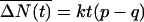and a variance of 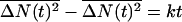, where I_v(x) is the modified Bessel function of the first kind and order v.

The thermodynamic information contained in the forward hopping probability p(z) can now be used to predict the nonequilibrium flow rate through a self-consistent differential equation, nQ = -ρ₀ Aż(t) = nk[2p(z) - 1], where n = 8 is the number of tubes connecting the two compartments. For a quadratic approximation to the free energy G(z) (see below) as a function of CNT membrane separation, z(t) can be determined analytically, as shown in Fig. 3B. We estimate a hopping time τ = 1/k = 20 ps (average waiting time per hop) for the water chains in the random walk model independently from 5-ns simulations of single CNT membranes in water. With the corresponding hopping rate k of ≈50 per ns, we find excellent agreement of the theory with the water flow averaged over five independent simulations (see Fig. 3B). In addition, two expected standard deviations from the average flow cover the observed variations of individual nonequilibrium trajectories.

We further test the random walk model by studying the dependence of the water flow rate on the CNT length between 8.5 and 45 Å, exceeding those of biological lipid membranes. All CNTs fill completely with linear chains of water molecules and the hopping time τ varies by only ≈20% between 18 and 22 ps. Indeed, doubling the length of the CNT membranes hardly affects the water flow rate in the osmotic system, as shown in Fig. 3B, and predicted by the random walk model. This finding demonstrates that for single-file flow friction with the wall does not significantly slow down the water transport, corresponding to almost perfect slip boundary conditions in the CNT pore (4, 32, 33). The osmotic water flow is thus independent of channel length at least up to several nanometers and is limited mainly by particle entry and exit events.

The net average flow rate per tube is determined primarily by the thermodynamic driving force, Q = k(p - q) = k tanh(-βΔμ/2), and limited by the hopping rate k, i.e.,|Q| ≤ k. For CNTs, k depends only weakly on the tube length. To compare the water flow rates through the CNT membranes and the protein aquaporin-1, we correct for a different osmolality ratio of 1.2 between the inside and outside of the liposomes in the measurements (28). In an ideal osmotic setup, the chemical potential difference is given by the concentration ratio ρ₁ and ρ₂ on the two sides of the membrane, exp(-Δμ/k_BT) = ρ₁/ρ₂, and the flow rate per channel becomes Q = k(1 - ρ₂/ρ₁)/(1 + ρ₂/ρ₁). Our hopping rate k and a density ratio of 1.2 would give a net transport of 4.5 water molecules per ns and pore, comparable to the measured value of 3.9 ± 0.6 ns^-1 for aquaporin-1 (28). The aquaporin-1 family of proteins has been studied extensively by MD (34, 35). Comparable flow rates were observed in a recent simulation (36), in which a flow was generated by external forces acting on water molecules to mimic the osmotic gradient in biological systems.

The fluid reservoirs in our simulations are finite, and after the water compartment shrinks to a width of ≈1 nm, water efflux occurs in distinct steps, marked by horizontal lines in Fig. 3A. The spacing of these steps is ≈3 Å, roughly corresponding to the diameter of a water molecule (Fig. 3C). Indeed, water molecules form layers parallel to the CNT membrane surfaces (Fig. 3C). In all five runs, two metastable layers form; in two of the five runs (Fig. 3A), one of the two layers breaks after several nanoseconds, and net water efflux stops with a water monolayer remaining. In neither of these two runs, this single sheet of water breaks, persisting for >50 ns in one of them. This finding is remarkable because complete dehydration of the nonpolar and porous CNT membranes and their subsequent association is thermodynamically strongly favored (Fig. 4, see below). Previous studies indeed indicate that breaking structured liquids confined by rigid surfaces is a slow process (37-40). Nanometer-thick films confined between polar and nonpolar surfaces in water were studied experimentally (41). The frequency-dependent response to shear suggested a “flickering vapor phase” with characteristic lifetimes of ≈100 s. Here, we find that breaking a water monolayer is slow on molecular time scales even for confining interfaces that can move freely and contain multiple and closely spaced pores for water efflux.

The apparent stability of layered water structures can be quantified by calculating the free energy G(z) as a function of CNT membrane separation from umbrella sampling. Fig. 4 shows the free energy profiles for both the NaCl water osmotic setup and a nonosmotic setup in which CNT membranes separate two pure-water compartments. As expected, for z ≥ 8 Å, the mean force, -G′(z), is essentially zero in the nonosmotic setup, whereas it is attractive in the osmotic setup (≈35 pN/nm², with a membrane unit area of ≈1.1 nm² per nanotube). Despite approximations in the intermolecular potentials and possibly significant interfacial effects, the free energies from experimental osmotic pressures are in good agreement with the simulation data for sufficiently large CNT membrane separations, z >8 Å (Fig. 4 Inset). In particular, the osmotic pressure, G′(z)/A, estimated from simulations to be ≈430 bar (for 5.64 M NaCl solution at z ≈18 Å) is only slightly higher (≈15%) than the corresponding experimental osmotic pressure of 380 bar.

At subnanometer separations, the molecularity and layering of water molecules is evident from large oscillations in the free energy profiles (Fig. 4). The corresponding forces, -G′(z), reach peaks of up to 400 pN per nm² of membrane area. Two distinct troughs at CNT membrane separations of 6.5 and 3.4 Å in Fig. 4 correspond to the formation of metastable double and single layers of water molecules confined between the membranes, respectively. Breaking successive water layers (3→2 and 2→1) lowers the overall free energy, although that gain is marginal compared with breaking the final layer of water. Complete drying and association of the two CNT membranes provides free energy gains of 150-200 kJ·mol^-1, or ≈60-80 k_BT, resulting in a thermodynamically stable contact between the CNT membranes.

Once formed, breaking the contact between membrane surfaces requires large external forces. The free energy profile in Fig. 4 indicates that upon breaking the contact by external force, water should fill the gap between the membranes by reverse osmosis. Indeed, when we use an external force to pull the two CNT membranes apart starting from the dry contact interface, water molecules flow from the salt solution into the initially empty water compartment to reform the molecular sheet on a subnanosecond membrane time scale. This finding suggests that a narrow slit between the CNT membranes kept at a height of ≈3 Å is filled at equilibrium by a water monolayer.

The layering of water is evident in the density profiles of water perpendicular to the membrane surface shown in Fig. 5. The five curves in Fig. 5 show the density profiles at membrane separations corresponding to five to one molecular diameters of water obtained from umbrella sampling simulations. These separations are identified by five horizontal lines in Fig. 3A. The region corresponding to the pure-water compartment is centered at the origin. The oscillations in the water density profiles show formation of distinct hydration layers parallel to the membrane surface. We find that the magnitude of these peaks increases upon reduction of molecular layers from five to one. Formation of similar solvation layers of water have also been observed experimentally in measurements of “hydration forces” between surfaces (42) and recently for xenon confined between flat surfaces (43).

Fig. 5.

Average water density (thick line) along the direction normal to the CNT membranes for different membrane-membrane separations corresponding to five to one layers of water molecules (top to bottom). The shaded and light regions correspond to the solvent-filled compartments and nanotube membranes, respectively. The pure water compartment is centered at z = 0. The thin horizontal lines indicate the bulk density of water.

Why are the 2D sheets of water so stable? One may expect that any fluctuation depleting the number of water molecules would weaken the sheet locally, and the remaining water molecules would then rapidly flow out into the salt compartment, thereby reducing the overall free energy by 60-80 k_BT. Instead, such fluctuations appear to be strongly suppressed. Water molecules in the layer form well-ordered networks of hydrogen bonds in the overall hydrophobic environment. The time-averaged density of water oxygens shows formation of well-defined inner and outer hydrogen-bonded rings comprising 6 and 12 water molecules, respectively, that line the pore and the rim of tubes and fill the interstitial spaces (Fig. 6). Most water molecules adopt orientations that lead to the formation of a large number of in-plane hydrogen bonds (close to three per water molecule), leading to the metastability of the one-layer structure. Interestingly, despite this tight network structure, water molecules in the 2D sheet remain fluid and exchange continuously with the saltwater compartment by flowing through the CNTs. We find that the in-plane diffusion coefficient is about half that of transferable intermolecular potential 3 point (TIP3P) water (23) in the bulk phase and comparable to that of single-file TIP3P water in a short CNT (19, 30). Qualitatively similar dynamics of water molecules in confined environments have been observed in recent experiments (44). These results point to the remarkable ability of water molecules to form fluctuating hydrogen-bond networks that can conform to a variety of 1D and 2D confined environments (45). For CNT membranes with significantly larger areas than those studied here capillary waves may become important and could induce local puncturing of the water sheet, nucleating a subsequent emptying process more readily. Nevertheless, the observed metastability of molecularly thin water layers is likely relevant in protein-protein encounters or other (bio)molecular interfaces.

Fig. 6.

(A) Average density of water oxygens in a water monolayer that lies parallel to the CNT membranes, color-coded in units of molecules per ų, where 0.033 Å^-3 is the bulk density of water. CNT cylinder axes are perpendicular to the plane and pass through the centers of the inner rings. (B) MD snapshot of water molecules that form the inner (green) and outer (red) hydrogen-bonded rings lining the pore and the outer rim of the CNTs. The center water molecule (blue) is located below the sheet and inside the CNT.

Conclusions

We show that water molecules flow through membranes of open-ended CNTs under an osmotic gradient. The resulting single-file water flow is almost friction-less and governed by microscopic fluctuations. A continuous-time random walk quantitatively describes the transport of water molecules, a process similar to polymer translocation through a pore (31). The observed flow rates of about five water molecules per ns and CNT are comparable to those measured for biological water channels (28) and almost independent of the tube length.

With fast “slip flow” (33), narrow channels can accommodate high flow rates essential for nanofluidics devices (4). Fluid-flow networks can be constructed by connecting the rigid cylindrical pores of CNTs with branched and tapered junctions (46-48). Simple nanotube assemblies have already been used as nanofiltration devices (5, 6). These developments suggest exciting opportunities for using nanotube networks and assemblies for controlled transport of water (14-19, 49-51), small molecules, and (bio)polymers, with possible applications in nanofluidics devices, desalination by reverse osmosis, and fuel cell devices.

References

- 1.Volkmuth, W. D. & Austin, R. H. (1992) Nature 358, 600-602. [DOI] [PubMed] [Google Scholar]
- 2.Gau, H., Herminghaus, S., Lenz, P. & Lipowsky, R. (1999) Science 283, 46-49. [DOI] [PubMed] [Google Scholar]
- 3.Prins, M. W. J., Welters, W. J. J. & Weekamp, J. W. (2001) Science 291, 277-280. [DOI] [PubMed] [Google Scholar]
- 4.Whitesides, G. M. & Stroock, A. D. (2001) Phys. Today 54, 42-48. [Google Scholar]
- 5.Jirage, K. B., Hulteen, J. C. & Martin, C. R. (1997) Science 278, 655-658. [Google Scholar]
- 6.Miller, S. A., Young, V. Y. & Martin, C. R. (2001) J. Am. Chem. Soc. 123, 12335-12342. [DOI] [PubMed] [Google Scholar]
- 7.Mitchell, D. T., Lee, S. B., Trofin, L., Li, N., Nevanen, T. K., Soderlund, H. & Martin, C. R. (2002) J. Am. Chem. Soc. 124, 11864-11865. [DOI] [PubMed] [Google Scholar]
- 8.Dujardin, E., Ebbeson, T. W., Hiura, H. & Tanigaki, K. (1994) Science 265, 1850-1852. [DOI] [PubMed] [Google Scholar]
- 9.Wong, S. S., Joselevich, E., Woolley, A. T., Cheung, C. L. & Lieber, C. M. (1998) Nature 394, 52-55. [DOI] [PubMed] [Google Scholar]
- 10.Deamer, D. W. & Akeson, M. (2000) Trends Biotechnol. 18, 147-151. [DOI] [PubMed] [Google Scholar]
- 11.Ajayan, P. M. & Iijima, S. (1993) Nature 361, 333-334. [Google Scholar]
- 12.Ajayan, P. M., Stephan, O., Redlich, P. & Colliex, C. (1995) Nature 375, 564-567. [Google Scholar]
- 13.Skoulidas, A. I., Ackerman, D. M., Johnson, J. K. & Sholl, D. S. (2002) Phys. Rev. Lett. 89, 185901. [DOI] [PubMed] [Google Scholar]
- 14.Gogotsi, Y., Libera, J. A., Guvenc-Yazicioglu, A. & Megaridis, C. M. (2001) Appl. Phys. Lett. 79, 1021-1023. [Google Scholar]
- 15.Koga, K., Gao, G. T., Tanaka, H. & Zeng, X. C. (2001) Nature 412, 802-805. [DOI] [PubMed] [Google Scholar]
- 16.Gordillo, M. C. & Martií, J. (2000) Chem. Phys. Lett. 329, 341-345. [Google Scholar]
- 17.Beckstein, O., Biggin, P. C. & Sansom, M. S. P. (2001) J. Phys. Chem. 105, 12902-12905. [Google Scholar]
- 18.Allen, R., Melchionna, S. & Hansen, J. P. (2002) Phys. Rev. Lett. 89, 175502. [DOI] [PubMed] [Google Scholar]
- 19.Hummer, G., Rasaiah, J. C. & Noworyta, J. P. (2001) Nature 414, 188-190. [DOI] [PubMed] [Google Scholar]
- 20.Murad, S. & Powles, J. G. (1993) J. Chem. Phys. 99, 7271-7272. [Google Scholar]
- 21.Pearlman, D. A., Case, D. A., Caldwell, J. W., Ross, W. S., Cheatham, T. E., Debolt, S., Ferguson, D., Seibel, G. & Kollman, P. (1995) Comput. Phys. Commun. 91, 1-41. [Google Scholar]
- 22.Cornell, W. D., Cieplak, P., Bayly, C. I., Gould, I. R., Merz, K. M., Ferguson, D. M., Spellmeyer, D. C., Fox, T., Caldwell, J. W. & Kollman, P. A. (1995) J. Am. Chem. Soc. 117, 5179-5197. [Google Scholar]
- 23.Jorgensen, W. L., Chandrasekhar, J., Madura, J. D., Impey, R. W. & Klein, M. L. (1983) J. Chem. Phys. 79, 926-935. [Google Scholar]
- 24.Straatsma, T. P. & Berendsen, H. J. C. (1988) J. Chem. Phys. 89, 5876-5886. [Google Scholar]
- 25.Berendsen, H. J. C., Postma, J. P. M., van Gunsteren, W. F., DiNola, A. & Haak, J. R. (1984) J. Chem. Phys. 81, 3684-3690. [Google Scholar]
- 26.Darden, T., York, D. & Pedersen, L. (1993) J. Chem. Phys. 98, 10089-10092. [Google Scholar]
- 27.Ferrenberg, A. M. & Swendsen, R. H. (1989) Phys. Rev. Lett. 63, 1195-1198. [DOI] [PubMed] [Google Scholar]
- 28.Zeidel, M. L., Ambudkar, S. V., Smith, B. L. & Agre, P. (1992) Biochemistry 31, 7436-7440. [DOI] [PubMed] [Google Scholar]
- 29.Levitt, D. G. (1973) Phys. Rev. A At. Mol. Opt. Phys. 8, 3050-3054. [Google Scholar]
- 30.Berezhkovskii, A. & Hummer, G. (2002) Phys. Rev. Lett. 89, 064503-064507. [DOI] [PubMed] [Google Scholar]
- 31.Muthukumar, M. (1999) J. Chem. Phys. 111, 10371-10374. [Google Scholar]
- 32.Zwanzig, R. (1978) J. Chem. Phys. 68, 4325-4326. [Google Scholar]
- 33.Pit, R., Hervet, H. & Léger, L. (2000) Phys. Rev. Lett. 85, 980-983. [DOI] [PubMed] [Google Scholar]
- 34.De Groot, B. L. & Grubmu̇ller, H. (2001) Science 294, 2353-2357. [DOI] [PubMed] [Google Scholar]
- 35.Tajkhorshid, E., Nollert, P., Jensen, M. O., Miercke, L. J. W., O'Connell, J., Stroud, R. M. & Schulten, K. (2002) Science 296, 525-530. [DOI] [PubMed] [Google Scholar]
- 36.Zhu, F. Q., Tajkhorshid, E. & Schulten, K. (2002) Biophys. J. 83, 154-160. [DOI] [PMC free article] [PubMed] [Google Scholar]
- 37.Lum, K. & Luzar, A. (1997) Phys. Rev. E 56, R6283-R6286. [Google Scholar]
- 38.Lum, K. & Chandler, D. (1998) Int. J. Thermophys. 19, 845-855. [Google Scholar]
- 39.Bolhuis, P. G. & Chandler, D. (2000) J. Chem. Phys. 113, 8154-8160. [Google Scholar]
- 40.Bratko, D., Curtis, R. A., Blanch, H. W. & Prausnitz, J. M. (2001) J. Chem. Phys. 115, 3873-3877. [Google Scholar]
- 41.Zhang, X., Zhu, Y. & Granick, S. (2002) Science 295, 663-666. [DOI] [PubMed] [Google Scholar]
- 42.Israelachvili, J. & Wennerstrom, H. (1996) Nature 379, 219-225. [DOI] [PubMed] [Google Scholar]
- 43.Donnelly, S. E., Birtcher, R. C., Allen, C. W., Morrison, I., Furuya, K., Song, M. H., Mitsuishi, K. & Dahmen, U. (2002) Science 296, 507-510. [DOI] [PubMed] [Google Scholar]
- 44.Raviv, U., Laurat, P. & Klein, J. (2001) Nature 413, 51-54. [DOI] [PubMed] [Google Scholar]
- 45.Cheng, Y. K. & Rossky, P. J. (1998) Nature 392, 696-699. [DOI] [PubMed] [Google Scholar]
- 46.Zhou, D. & Seraphin, S. (1995) Chem. Phys. Lett. 238, 286-289. [Google Scholar]
- 47.Li, J., Papadopoulos, C. & Xu, J. (1999) Nature 402, 253-254.10580494 [Google Scholar]
- 48.Huang, Y., Duan, X. F., Wei, Q. Q. & Lieber, C. M. (2001) Science 291, 630-633. [DOI] [PubMed] [Google Scholar]
- 49.Walther, J. B., Jaffe, R., Halicioglu, T. & Koumoutsakos, P. (2001) J. Phys. Chem. 105, 9980-9987. [Google Scholar]
- 50.Maibaum, L. & Chandler, D. (2003) J. Phys. Chem. 107, 1189-1193. [Google Scholar]
- 51.Zhu, F. & Schulten, K. (2003) Biophys. J. 85, 236-244. [DOI] [PMC free article] [PubMed] [Google Scholar]