Optical Coherence Tomography Machine Learning Classifiers for Glaucoma Detection: A Preliminary Study

Abstract

Purpose

Machine-learning classifiers are trained computerized systems with the ability to detect the relationship between multiple input parameters and a diagnosis. The present study investigated whether the use of machine-learning classifiers improves optical coherence tomography (OCT) glaucoma detection.

Methods

Forty-seven patients with glaucoma (47 eyes) and 42 healthy subjects (42 eyes) were included in this cross-sectional study. Of the glaucoma patients, 27 had early disease (visual field mean deviation [MD] ≥ −6 dB) and 20 had advanced glaucoma (MD < −6 dB). Machine-learning classifiers were trained to discriminate between glaucomatous and healthy eyes using parameters derived from OCT output. The classifiers were trained with all 38 parameters as well as with only 8 parameters that correlated best with the visual field MD. Five classifiers were tested: linear discriminant analysis, support vector machine, recursive partitioning and regression tree, generalized linear model, and generalized additive model. For the last two classifiers, a backward feature selection was used to find the minimal number of parameters that resulted in the best and most simple prediction. The cross-validated receiver operating characteristic (ROC) curve and accuracies were calculated.

Results

The largest area under the ROC curve (AROC) for glaucoma detection was achieved with the support vector machine using eight parameters (0.981). The sensitivity at 80% and 95% specificity was 97.9% and 92.5%, respectively. This classifier also performed best when judged by cross-validated accuracy (0.966). The best classification between early glaucoma and advanced glaucoma was obtained with the generalized additive model using only three parameters (AROC = 0.854).

Conclusions

Automated machine classifiers of OCT data might be useful for enhancing the utility of this technology for detecting glaucomatous abnormality.

Glaucoma is an optic neuropathy characterized by a gradual loss of retinal ganglion cells and thinning of the retinal nerve fiber layer (RNFL).^1,2 The functional assessment of glaucoma damage is determined by visual field (VF) testing. Glaucomatous VF abnormality is detectable only after significant RNFL loss has already occurred.³ In addition, VF testing is prone to short- and long-term fluctuations and thus multiple testing is required to confirm any abnormalities. Assessment of the optic nerve head (ONH) and the peripapillary RNFL can provide earlier indications of glaucomatous damage.^4–6 However, the wide range of normal anatomic variation and the subjective nature of clinical examination limit their reliability. An objective method of measuring the optic nerve structure and RNFL thickness has a significant diagnostic value.

Optical coherence tomography (OCT) is a noncontact, non-invasive imaging technology that uses light to create high-resolution, cross-sectional tomographic images of the retina and the ONH.⁷ The device differentiates layers in the retina due to the differences in time delay of reflection from various components of the tissue. Previous studies have shown that OCT data are highly reproducible,^8–11 and that the device has the capability to differentiate glaucomatous from nonglaucomatous eyes.^12–16

Since OCT provides numerous stereometric measurements of the disc, macula and peripapillary RNFL, it is important to find the parameters that serve best in the detection of glaucoma. Previous experience with confocal scanning laser oph-thalmoscopy^17,18 and scanning laser polarimetry^19,20 showed that the combination of multiple parameters and advanced data analysis methods can improve the sensitivity and specificity of glaucoma detection. Specifically, improved discrimination between glaucomatous and healthy eyes was obtained with machine-learning classifiers.^21–24

Machine-learning classifiers are trained computerized systems with the ability to detect the relationship between multiple input parameters and a diagnosis. Trained classifiers can be used to predict the diagnosis of new cases. The purpose of this cross-sectional study was to test the performance of numerous machine-learning techniques using OCT data to discriminate between glaucomatous and healthy eyes.

Methods

Subjects

We enrolled healthy subjects and glaucoma patients meeting eligibility criteria to this cross-sectional study. The study was approved by the Institutional Review Board/Ethics Committee, and adhered to the Declaration of Helsinki and Health Insurance Portability and Accountability Act regulations, with informed consent obtained from all participants.

All subjects had a comprehensive ophthalmic evaluation, and all tests were completed within six months. The evaluation included medical history, best-corrected visual acuity, manifest refraction, intraocular pressure (IOP) measurements by Goldmann applanation, gonioscopy, slit-lamp examination before and after pupil dilation, VF testing, and OCT scanning of the disc, macula, and peripapillary RNFL. All subjects underwent pupillary dilation with 1% tropicamide and 2.5% phenylephrine, both from Alcon Laboratories, Inc. (Fort Worth, TX).

All the participants had best-corrected visual acuity of 20/40 or better and refractive error between −6.00 and +6.00 diopters (D; spherical equivalent). Subjects were excluded if they exhibited signs of retinal or ONH pathologies other than glaucoma, if media opacity or a poorly dilating pupil interfered with clinical viewing or imaging of the fundus, or if they chronically used medications that are known to affect retinal thickness. Patients were also excluded if they had systemic diseases that might affect the retina or VF or if they had any previous operation in the study eye other than uneventful cataract extraction.

Glaucomatous Eyes

Eyes were defined as glaucomatous if there was both glaucomatous optic neuropathy (GON) and glaucomatous VF loss. GON was defined as either intereye cup-disc ratio asymmetry > 0.2, accounting for disc size; rim thinning or notching; peripapillary hemorrhages; or cup-disc ratio ≥ 0.6. Glaucomatous VF loss was diagnosed if any of the following findings were evident on two consecutive VF tests: a glaucoma hemifield test outside normal limits, pattern standard deviation (PSD) < 5%, or a cluster of three or more nonedge points in typical glaucomatous locations, all depressed on the pattern deviation plot at a level of P < 0.05, with one point in the cluster depressed at a level of P < 0.01.

Healthy Eyes

Eyes were defined as healthy if there was no history or evidence of glaucoma, IOP ≤ 21 mm Hg, ONH not meeting the criteria for GON as previously described, and a normal Humphrey 24–2–pattern VF not meeting the criteria for glaucomatous VF loss as previously described.

VF Testing

All subjects underwent Humphrey Swedish interactive thresholding algorithm standard or full-threshold 24–2 perimetry (Carl Zeiss Meditec, Dublin, CA). A reliable VF test was defined as one with fewer than 30% fixation losses, false-positive, or false-negative responses. The VF results were considered reproducible if the same type, location, and index of abnormality were evident in two consecutive VF tests.

OCT Scanning

All OCT scans were performed using commercially available equipment (Stratus OCT with software version 2.0; Carl Zeiss Meditec) with an in vivo tissue resolution of approximately 8 to 10 μm.

OCT measurements of the macula were generated with a fast protocol of six 6-mm linear scans in a spoke pattern configuration centered on the fovea, lines 30° apart. OCT measurements of the ONH were done with a fast protocol in a similar spoke pattern. Peripapillary RNFL scans were done with a fast protocol of three circumpapillary scans centered on the ONH with a diameter of 3.4 mm.

Scans were defined as poor quality if the signal-noise ratio was below 35 dB and/or there was overt misalignment of the surface detection algorithm of at least 15% consecutively or 20% cumulatively of the total sampling points. All OCT data were aligned according to the orientation of the right eye. In this way, clock hour 9 of the circumpapillary scan represented the temporal aspect of the ONH for both eyes.

Thirty-eight OCT parameters, which all appear in the conventional printouts, were used for the analysis. From the macular scan, we used retinal thickness in nine sectors as well as macular volume. We also used the global mean macular thickness, which was derived from a weighted mean of the regional measurements taking into account the relative area of each sector, as described previously.²⁵ From the ONH scans, we used all 10 parameters: vertical integrated rim area, horizontal integrated rim width, disc area, cup area, rim area, cup-disc–area ratio, horizontal cup-disc ratio, vertical cup-disc ratio, cup area (topographic), and cup volume (topographic). Circumpapillary analysis resulted in an additional 17 parameters: global mean RNFL thickness, 4 quadrant mean thicknesses, and 12 clock hour means.

Machine Classifiers

The following classifying methods were tested: linear discriminant analysis (LDA), generalized linear model (GLM), and generalized additive model (GAM). In addition, the following machine learning classifiers were tested: support vector machine (SVM) and recursive partitioning and regression tree (RPART). All classifiers were implemented in the statistical software (R version 1.9; R-Project, available at http://cran.r-project.org).

LDA assumes a Gaussian distribution of data and defines linear discrimination boundaries between the categories where it maximizes the variance between classes while minimizing the variance within classes. The classification of a new data point is determined by the likelihood that it is generated from each of the different categories.^26,27

GLM assumes that the log of the odds ratio of a patient having glaucoma versus being healthy can be expressed as a linear function of the parameters.²⁸ The decision boundary between glaucomatous and healthy eyes is the hyperplane where the predicted odds of a patient having glaucoma are equal to the predicted odds of the same patient being healthy.

GAM assumes that the conditional expectation of glaucoma severity given by OCT parameters (unchanged) can be expressed as a sum of univariate smooth functions of the OCT parameters.²⁹ The fitted model minimizes mean squared prediction error subject to certain penalty of model complexity.

SVMs map multidimensional input space into a high-dimensional feature space.^30,31 In this feature space, the classifier finds the hyper-plane separating glaucomatous from healthy eyes that maximizes the distance of any case from the hyperplane. The transformation of input space to feature space is called a kernel; in this study a linear kernel was used. The SVM used in this study also allowed for imperfect classification of glaucomatous and healthy eyes by the algorithm in situations where perfect classification is not possible. Intuitively, this makes the classification correct for testing data that is near but not identical to the training data.

The RPART function is an implementation of the decision-tree algorithm. It recursively partitions the parameter space along some of the parameters.³² The partition process can be represented by a binary tree, and the partitioned regions of the parameter space are called leaves. The choice of the parameters to be split and the points at which the parameter space is split are chosen to maximize certain scores, such as information gain. A new case is classified using majority vote of cases in the training data belonging to the same leaf as the new case.

Feature Selection

The classification was performed using all 38 available parameters and with 8 parameters with the highest correlation with VF mean deviation (MD). A limited number of parameters was used to ensure the reliability of the machine classifiers accounting for the limited study sample size. A backward selection using Akaike information criteria (AIC) from these eight parameters was used to further simplify the classifier formula with preservation of the discrimination capabilities. Backward feature selection could not be used for SVM and RPART, for which AIC is not defined, and for LDA, in which the AIC is not reliable.

Data Analysis and Statistics

The study population characteristics were compared using Student’s t-test for continuous parameters and a χ² test for categorical parameters (JMP software; SAS Institute, Cary, NC).

Receiver operating characteristic (ROC) curves were used to describe the ability of the classifier to differentiate between glaucomatous and healthy eyes. ROC was calculated for each individual parameter. To get an unbiased estimate of the ROC curves, all 89 patients were divided into six equal groups (one patient appears in two groups). Six tests were conducted for each classifier; in each test, a different group of patients was chosen to be the testing set. The other five groups were used as training sets. ROC was calculated for each of the tests, and the final cross-validation ROC curve was computed as the pointwise average of the six ROC curves. The area under the ROCs (AROCs) for the six folds across algorithms were compared using the DeLong method.³³ The sensitivity was calculated at the arbitrary specificities of 80% and 95%.

Cross-validation accuracy was used to estimate the ability of the different classifiers to discriminate between glaucomatous and healthy eyes.^34,35 The accuracy was the number of true predictions out of the total number of observations. In this method, the model is created on all the data except one eye as a training set, then testing is performed on the remaining eye and reported with accuracy. This is repeated a number of times equal to the number of eyes tested, and the accuracies are averaged. This way of cross-validation maximizes utilization of the data set for creating the model.

RESULTS

Subject Characteristics

One hundred sixty-one consecutive patients from the glaucoma clinic were evaluated for this study. Seven were excluded due to diabetes, three had eye diseases that caused media opacity, three had age-related macular degeneration, eight had refractive error exceeding 6 D, and one had visual acuity below 20/40. In addition, 36 had only one VF test, and 8 had a nonreliable VF test. Among the 95 qualified subjects, only 63 eyes met both GON and VF criteria. Sixteen more eyes were excluded due to poor OCT scans (6 ONH, 7 macula, and 3 NFL).

Seventy-five healthy volunteers were recruited. Among them, three had visual acuity below 20/40, two had diabetes, three had myopia exceeding 6 D, and five had a nonreliable VF test. Among the qualified healthy volunteers, 52 had both normal VF and normal ONH appearance. Ten more subjects were excluded due to poor scans (5 ONH, 4 macula and 1 NFL).

Eyes of 42 healthy subjects (42 healthy eyes) and 47 glaucoma patients meeting eligibility criteria (47 glaucomatous eyes) were analyzed in this study. The study population characteristics are summarized in Table 1. The healthy subjects were significantly younger than the glaucoma patients (P = 0.001), and the mean VF MD of the glaucomatous eyes was −6.4 ± 5.0 dB.

Table 1.

Characteristics of the Study Population

		Glaucomatous Eyes
Characteristic	Healthy Eyes (n = 42)	Early (n = 27)	Advanced (n = 20)	P
Age (years)	53.6 ± 18.6 (21.1 to 98.8)	64.4 ± 12.7 (27.3 to 81.8)	65.5 ± 11.8 (41.9 to 87.5)	0.005*
Race
White	33	23	13	NA
African-American	8	2	4
Asian	1	2	3
Male/female	23/19	11/16	9/11	0.5†
MD (dB)	0.1 ± 0.9 (−2.3 to 1.7)	−2.8 ± 1.8 (−5.6 to −0.2)	−10.9 ± 4.2 (−19.8 to −6.1)	< 0.001*
PSD (dB)	1.4 ± 0.2 (1.1 to 1.9)	5.0 ± 2.0 (1.8 to 10.8)	10.0 ± 2.9 (4.1 to 14.5)	< 0.001*

Values are n or means ± SD (range). NA, not applicable; MD, mean deviation; PSD, pattern standard deviation.

^*ANOVA.

^†χ².

Discriminating between Glaucomatous and Healthy Eyes

Using individual OCT parameters, the largest AROC among the ONH parameters was found for rim area (0.969); among the circumpapillary parameters, the mean NFL (0.938); and among the macular scanning parameters, the overall mean macular thickness (0.839) (Table 2). Using all 38 parameters, the largest AROC was achieved with SVM (0.948), followed by LDA (0.902). The accuracy and sensitivity for the individual best parameters and for the classifiers using all parameters were similar. The analysis was repeated using only eight parameters that had the best correlation with VF MD (Table 3). The use of only eight parameters increased the AROC for all three classifiers to a range of 0.885 to 0.981 (Table 2, Fig. 1). The sensitivity of both SVM and LDA using eight parameters (SVM[8] and LDA[8]) at a specificity of 80% was 97.9%, and the sensitivity at 95% specificity was 92.5% and 91.2%, respectively. Backward elimination was used with the GLM method; four parameters (GLM[4]; Table 3) were found to provide the largest AROC (0.975) (Table 2, Fig. 1).

Table 2.

AROC, Accuracy, and Sensitivity at 80% and 95% Specificity for Differentiating between Healthy and Glaucomatous Eyes

			Sensitivity (%)
Classifier*	AROC	AROC SE	Specificity 80%	Specificity 95%	Accuracy
SVM(8)	0.981	0.033	97.9%	92.5%	0.966
LDA(8)	0.979	0.032	97.9%	91.2%	0.944
GLM(4)	0.975	0.033	95.8%	91.8%	0.955
SVM	0.948	0.056	94.6%	82.9%	0.910
LDA	0.902	0.060	86.3%	73.2%	0.831
RPART(8)	0.885	0.057	86.7%	57.2%	0.831
RPART	0.863	0.059	84.4%	46.8%	0.764
Rim area	0.969	0.036	92.9%	86.9%	0.899
Mean NFL	0.938	0.071	85.0%	80.6%	0.865
Mean macula	0.839	0.133	70.4%	57.8%	0.742

SE = standard error, SVM = support vector machine, SVM(8) = support vector machine using only 8 parameters, LDA = linear discriminant analysis, LDA(8) = linear discriminant analysis using only 8 parameters, RPART = recursive partitioning and regression tree, RPART(8) = recursive partitioning and regression tree using only 8 parameters, GLM(4) = generalized linear model using 4 parameters, NFL = nerve fiber layer.

^*Numbers in parentheses indicate number of parameters used.

Table 3.

OCT Parameters Used with the Various Classifiers

	Classifier*
Parameter	LDA(8)	RPART(8)	SVM(8)	GLM(4)	GAM(3)
HIRW	●	●	●		●
Rim area	●	●	●	●
HCDR					●
VCDR	●	●	●	●
Mean NFL	●	●	●
NFL inferior	●	●	●	●
NFL superior					●
NFL 6	●	●	●
NFL 7	●	●	●
NFL 11	●	●	●	●

HIRW, horizontal integrated rim width; HCDR, horizontal cup-disc ratio; VCDR, vertical cup-disc ratio.

^*Numbers in parentheses indicate number of parameters used.

Figure 1.

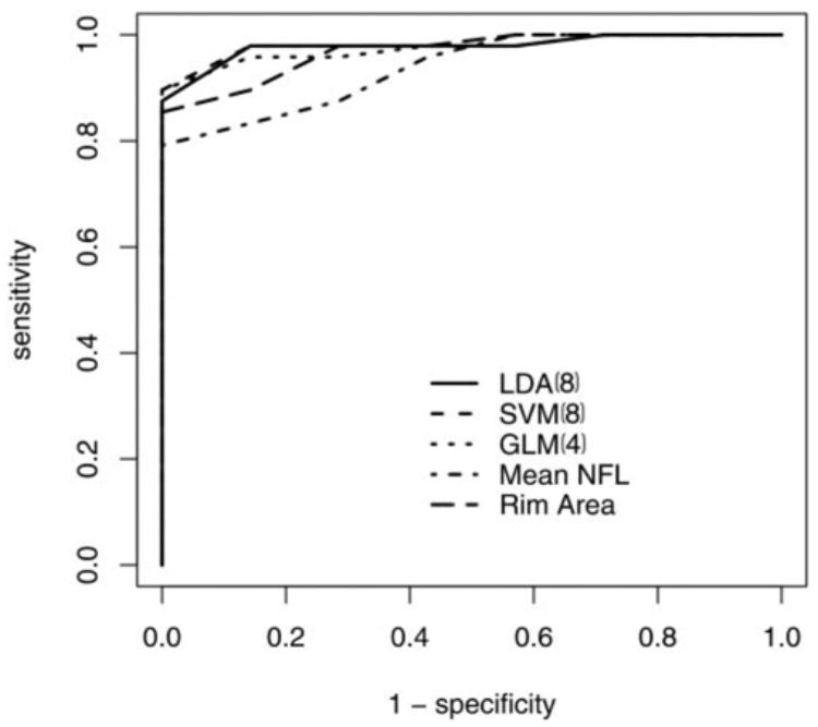
ROC curves of the best machine classifiers and best single parameters for discriminating between healthy and glaucomatous eyes.

Comparing the AROC of the classifiers with the single best parameters showed no significant difference with the rim area results. The AROC for SVM(8) was larger than the AROC for mean NFL (P = 0.05). SVM(8), LDA(8), GLM(4), and SVM had a significantly larger AROC than mean macular thickness (P < 0.05). The accuracy of SVM(8) was not significantly higher then that of rim area (P = 0.07). The accuracy of both SVM(8) and GLM(4) was significantly higher than that of mean NFL (P = 0.01 and 0.03, respectively). The accuracy of these classifiers as well as that of LDA(8) was significantly higher than that of mean macular thickness (P < 0.001).

Adding age as one of the attributes of the machine classifiers did not improve the prediction of the analysis. The sample size prevents drawing any conclusion about the importance of gender as a predictor.

Grading the Severity of Glaucoma

The glaucoma patients participating in this study were divided into those with early and late stages of disease, defining MD ≥ −6.0 dB as an indication of early glaucoma and MD < −6.0 dB as indicative of advanced glaucoma. Twenty-seven of the 47 patients were classified as having early glaucoma, whereas 20 had advanced glaucoma. Using machine classifiers, we noted a substantial reduction in the AROC for differentiating between early and advanced glaucoma compared to those found for differentiating between healthy and glaucomatous eyes. The best model to distinguish between these groups was GAM, using 3 of the 38 parameters that were tested (Table 3). The AROC was 0.854 and the accuracy of GAM(3) was 0.745. The model correlation coefficient with MD was 0.811 (P < 0.001, confidence interval −0.891–0.683; Fig. 2).

Figure 2.

Scatter plot of the output values of GAM and VF MD of 47 glaucoma patients

Discussion

We investigated the performance of computerized machine classifiers in discriminating between healthy and glaucomatous eyes using OCT parameters obtained from the macula, peripapillary, and ONH regions. The best classifier was SVM using only eight parameters (AROC 0.981 ± 0.033, accuracy 0.966), followed by LDA using eight parameters and GLM using only four parameters (Table 2). Both AROC and accuracy were higher for these machine classifiers than those obtained using the best single OCT parameter (rim area), though the difference was not significant. Given the high AROC of the single best parameter in this study group (0.969), significant improvement in discrimination capabilities is difficult to obtain. However, when comparing the ROC graphs (Fig. 1), the improved sensitivity of the machine classifiers is clearly seen in regions of highest specificity (upper left corner), which is the key location for a diagnostic tool. The improved performance was also evident when comparing the accuracy and sensitivity for the various specificities.

Our study population included a spectrum of glaucomatous damage that approximated the average glaucoma practice. In this population we found that even the use of a single parameter allowed for better differentiation between healthy and glaucomatous eyes than the majority of previously published studies.^{13,15,16,36,37} This might be due to the inclusion criteria used in our study. However, Buedenz et al.³⁸ have recently reported an AROC of 0.971 for an RNFL parameter similar to the findings in our study. Nouri-Mahdavi et al.³⁹ used logistic regression of numerous parameters, which did not significantly improve the discrimination between glaucoma and healthy subjects. Applying Fourier analysis to OCT circumpapillary data resulted in an AROC of 0.925.¹⁶ Hougaard et al.⁴⁰ used an NFL symmetry test on the RNFL scan data, which improved the sensitivity in detecting glaucoma compared to the best single parameter, but the difference was not significant.

We found that a limited number of parameters provided an improved differentiation between eyes. This in turn may allow implementation of these algorithms into OCT software for clinical use. Interestingly, all eight parameters used were acquired either in the ONH or the peripapillary regions, with no contribution from macular data.

We used two methods of cross-validation, sixfold and leave-one-out, to avoid training the classifiers and testing their performance on the same group. In sixfold cross-validation, the training is performed on five sixths and tested on the remaining sixth of the entire population. The procedure is repeated six times; thus, each group serves as a testing group one time. In the leave-one-out cross-validation, the training is done on the entire population, except one subject that is tested. This procedure is repeated multiple times, equal to the number of the participating subjects, and each time a single subject is tested. The cross-validated AROC and accuracy results thus provided unbiased estimates of the performance of the machine-learning classifiers trained with relatively small samples. It should be noted that with limited sample size, complex machine-learning classifiers such as SVM, LDA, or GLM tend to perform worse than simpler classifiers such as single OCT parameters. However, as sample size increases, complex classifiers tend to perform better. Our findings of improved cross-validated AROC and accuracy of the machine-learning classifiers compared with the single OCT parameters with only 89 participants is encouraging, although the one-side P-value for comparison with a single parameter only approached the significance level (P = 0.07). Nevertheless, these methods do not eliminate the possible confounder due to undetermined findings that might be exclusive to our study group. Therefore, it would be beneficial to test our models on a separate independent group of subjects.

Since glaucomatous damage can cause either local or generalized abnormalities, we used both segmental and global measurements with the machine classifiers (e.g., overall mean macula and segmental macular measurement). The eight selected parameters (Table 3) included overall NFL thickness, NFL thickness in the inferior quadrant, and NFL thickness at clock hours 6 and 7, which can be perceived as giving additional weight for the inferior sector as a typical location of glaucomatous damage.^{15,16,36–38}

Linear discriminating methods (LDA and GLM) could differentiate between groups in a capacity similar to the multidimensional discrimination method of SVM. This can be appreciated in Figure 3, where the multidimensional OCT data are projected onto a two-dimensional plane. It is easily observed that a linear plane can be placed between healthy and glaucomatous eyes.

Figure 3.

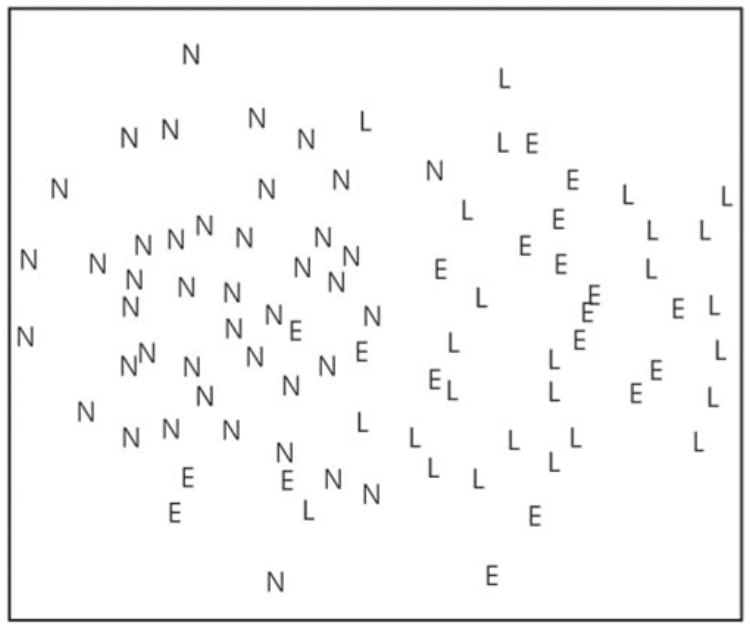
Two-dimensional mapping of the multidimensional OCT data used by the machine classifier. The distance between each data point in a 37-dimension machine classifier space is reduced to 2 dimensions in the illustration. Each eye is labeled according to the VF findings: E, early glaucoma (MD ≤ 6 dB); L, advanced glaucoma (MD > 6 dB); N, healthy (normal).

We further investigated the capability of machine classifiers to differentiate between early and advanced glaucoma. The best classification between early glaucoma and advanced glaucoma was obtained with GAM(3) (AROC = 0.854), which showed a good correlation with the MD on VF (r = .811, P < 0.0001). As shown in Figure 3, there was a substantial overlap between early and advanced glaucoma, which is reflected in lower discrimination capabilities than those observed between absence and presence of glaucoma. A possible explanation for the decreased discriminating ability is derived from the method we used to define the groups. While the diagnosis of glaucoma was based on a combination of structural and functional findings (GON and VF defect), the severity grading was defined solely by VF results. It is expected that a structural measure as obtained by OCT will have a better correspondence with combined structural-functional diagnosis than only functional assessment. Other studies have reported that correlation between the best OCT parameters and MD ranges between 0.47 and 0.729.^12,15,16 Since it has been postulated that structural glaucomatous changes may precede the appearance of functional changes^3,41,42 one cannot exclude the possibility that the machine classifier severity index gives a better evaluation of glaucoma severity than the VF MD. Moreover, the machine classifier method that we present might be mainly beneficial for longitudinal assessment of patients. Further investigation is required.

We found a significant difference in age between the healthy subjects and the patients with glaucoma. There was concern that if age was included as a parameter in the machine classifier model, it might unduly influence the outcome; overriding the parameters produced by the OCT. To test this, we added the age as an input parameter to the machine classifiers. The accuracy of the classifiers was not improved. Nevertheless, we did not use age as one of the attributes of the machine classifiers to avoid the possibility of biasing the results.

Another limitation of our study was the small sample size. This might affect the findings when using all 38 OCT printout data parameters. As was mentioned earlier, complex machine classifiers that use numerous input parameters tend to perform better in larger datasets. Further investigation with larger number of participants is currently underway.

In summary, machine classifiers of OCT measurements can provide a simple and accurate index for diagnosing the presence or absence of glaucoma as well as its severity. The classifiers that used a limited number of parameters (8) yielded the best discriminating capacity. A grading system for the severity of glaucoma was developed. A long-term prospective study is needed to determine the utility of this grading index in assessing glaucoma progression, compared to existing parameters.

References

- 1.Sommer A, Miller NR, Pollack I, et al. The nerve fiber layer in the diagnosis of glaucoma. Arch Ophthalmol. 1977;95:2149–2156. doi: 10.1001/archopht.1977.04450120055003. [DOI] [PubMed] [Google Scholar]
- 2.Harwerth RS, Carter-Dawson L, Shen F, et al. Ganglion cell losses underlying visual field defects from experimental glaucoma. Invest Ophthalmol Vis Sci. 1999;40:2242–2250. [PubMed] [Google Scholar]
- 3.Quigley HA, Addicks EM, Green WR. Optic nerve damage in human glaucoma. III. Quantitative correlation of nerve fiber loss and visual field defect in glaucoma, ischemic neuropathy, papilledema, and toxic neuropathy. Arch Ophthalmol. 1982;100:135–146. doi: 10.1001/archopht.1982.01030030137016. [DOI] [PubMed] [Google Scholar]
- 4.Sommer A, Katz J, Quigley HA, et al. Clinically detectable nerve fiber atrophy precedes the onset of glaucomatous field loss. Arch Ophthalmol. 1991;109:77–83. doi: 10.1001/archopht.1991.01080010079037. [DOI] [PubMed] [Google Scholar]
- 5.Quigley HA, Katz J, Derick RJ, et al. An evaluation of optic disc and nerve fiber layer examinations in monitoring progression of early glaucoma damage. Ophthalmology. 1992;99:19–28. doi: 10.1016/s0161-6420(92)32018-4. [DOI] [PubMed] [Google Scholar]
- 6.Wang F, Quigley HA, Tielsch JM. Screening for glaucoma in a medical clinic with photographs of the nerve fiber layer. Arch Ophthalmol. 1994;112:796–800. doi: 10.1001/archopht.1994.01090180094042. [DOI] [PubMed] [Google Scholar]
- 7.Huang D, Swanson EA, Lin CP, et al. Optical coherence tomography. Science. 1991;254:1178–1181. doi: 10.1126/science.1957169. [DOI] [PMC free article] [PubMed] [Google Scholar]
- 8.Schuman JS, Pedut-Kloizman T, Hertzmark E, et al. Reproducibility of nerve fiber layer thickness measurements using optical coherence tomography. Ophthalmology. 1996;103:1889–1898. doi: 10.1016/s0161-6420(96)30410-7. [DOI] [PMC free article] [PubMed] [Google Scholar]
- 9.Blumenthal EZ, Williams JM, Weinreb RN, et al. Reproducibility of nerve fiber layer thickness measurements by use of optical coherence tomography. Ophthalmology. 2000;107:2278–2282. doi: 10.1016/s0161-6420(00)00341-9. [DOI] [PubMed] [Google Scholar]
- 10.Villain MA, Greenfield DS. Peripapillary nerve fiber layer thickness measurement reproducibility using optical coherence tomography. Ophthalmic Surg Lasers Imaging. 2003;34:33–37. [PubMed] [Google Scholar]
- 11.Paunescu LA, Schuman JS, Price LL, et al. Reproducibility of nerve fiber thickness, macular thickness, and optic nerve head measurements using StratusOCT. Invest Ophthalmol Vis Sci. 2004;45:1716–1724. doi: 10.1167/iovs.03-0514. [DOI] [PMC free article] [PubMed] [Google Scholar]
- 12.Hoh ST, Greenfield DS, Mistlberger A, et al. Optical coherence tomography and scanning laser polarimetry in normal, ocular hypertensive, and glaucomatous eyes. Am J Ophthalmol. 2000;129:129–135. doi: 10.1016/s0002-9394(99)00294-9. [DOI] [PubMed] [Google Scholar]
- 13.Bowd C, Zangwill LM, Berry CC, et al. Detecting early glaucoma by assessment of retinal nerve fiber layer thickness and visual function. Invest Ophthalmol Vis Sci. 2001;42:1993–2003. [PubMed] [Google Scholar]
- 14.Guedes V, Schuman JS, Hertzmark E, et al. Optical coherence tomography measurement of macular and nerve fiber layer thickness in normal and glaucomatous human eyes. Ophthalmol. 2003;110:177–189. doi: 10.1016/s0161-6420(02)01564-6. [DOI] [PMC free article] [PubMed] [Google Scholar]
- 15.Kanamori A, Nakamura M, Escano MF, et al. Evaluation of the glaucomatous damage on retinal nerve fiber layer thickness measured by optical coherence tomography. Am J Ophthalmol. 2003;135:513–520. doi: 10.1016/s0002-9394(02)02003-2. [DOI] [PubMed] [Google Scholar]
- 16.Essock EA, Sinai MJ, Bowd C, et al. Fourier analysis of optical coherence tomography and scanning laser polarimetry retinal nerve fiber layer measurements in the diagnosis of glaucoma. Arch Ophthalmol. 2003;121:1238–1245. doi: 10.1001/archopht.121.9.1238. [DOI] [PubMed] [Google Scholar]
- 17.Wollstein G, Garway-Heath DF, Hitchings RA. Identification of early glaucoma cases with the scanning laser ophthalmoscope. Ophthalmology. 1998;105:1557–1563. doi: 10.1016/S0161-6420(98)98047-2. [DOI] [PubMed] [Google Scholar]
- 18.Mikelberg FS, Parfitt CM, Swindale NV, et al. Ability of the Heidelberg retina tomograph to detect early glaucomatous visual field loss. J Glaucoma. 1995;4:242–247. [PubMed] [Google Scholar]
- 19.Medeiros FA, Susanna R., Jr Comparison of algorithms for detection of localized nerve fiber layer defects using scanning laser polarimetry. Br J Ophthalmol. 2003;87:413–419. doi: 10.1136/bjo.87.4.413. [DOI] [PMC free article] [PubMed] [Google Scholar]
- 20.Colen TP, Tang NE, Mulder PG, Lemij HG. Sensitivity and specificity of new GDx parameters. J Glaucoma. 2004;13:28–33. doi: 10.1097/00061198-200402000-00006. [DOI] [PubMed] [Google Scholar]
- 21.Bowd C, Chan K, Zangwill LM, et al. Comparing neural networks and linear discriminant functions for glaucoma detection using confocal scanning laser ophthalmoscopy of the optic disc. Invest Ophthalmol Vis Sci. 2002;43:3444–3454. [PubMed] [Google Scholar]
- 22.Zangwill LM, Chan K, Bowd C, et al. Heidelberg retina tomograph measurements of the optic disc and parapapillary retina for detecting glaucoma analyzed by machine learning classifiers. Invest Ophthalmol Vis Sci. 2004;45:3144–3151. doi: 10.1167/iovs.04-0202. [DOI] [PMC free article] [PubMed] [Google Scholar]
- 23.Mardin CY, Hothorn T, Peters A, et al. New glaucoma classification method based on standard Heidelberg retina tomograph parameters by bagging classification tree. J Glaucoma. 2003;12:340–346. doi: 10.1097/00061198-200308000-00008. [DOI] [PubMed] [Google Scholar]
- 24.Lauande-Pimentel R, Carvalho RA, Oliveiar HC, et al. Discrimination between normal and glaucomatous eyes with visual field and scanning laser polarimetry measurements. Br J Ophthalmol. 2001;85:586–591. doi: 10.1136/bjo.85.5.586. [DOI] [PMC free article] [PubMed] [Google Scholar]
- 25.Wollstein G, Schuman JS, Price LL, et al. Optical coherence tomography (OCT) macular and peripapillary retinal nerve fiber layer measurements and automated visual fields. Am J Ophthalmol. 2004;138:218–225. doi: 10.1016/j.ajo.2004.03.019. [DOI] [PubMed] [Google Scholar]
- 26.Fisher R. The use of multiple measurements in taxonomic problems. Annals of Eugenics. 1936;7:179–188. [Google Scholar]
- 27.Hastie T, Tibshirani R, Friedman J. The Elements of Statistical Learning. New York: Springer; 2001. pp. 84–95. [Google Scholar]
- 28.Nelder JA, Wedderburn RWM. Generalized linear models. J R Stat Soc A. 1972;135:370–384. [Google Scholar]
- 29.Hastie T, Tibshirani R. Generalized additive models. Stat Sci. 1986;1:297–318. doi: 10.1177/096228029500400302. [DOI] [PubMed] [Google Scholar]
- 30.Vapnik V. Statistical Learning Theory. New York: Wiley-Interscience; 1998. pp. 401–441. [Google Scholar]
- 31.Schlkopf R, Smola A. Learning with Kernels: Support Vector Machines, Regularization, Optimization and Beyond. Cambridge, MA: MIT Press; 2001. pp. 189–222. [Google Scholar]
- 32.Breiman L, Friedman J, Olshen R, Stone C. Classification and Regression Trees. Belmont, CA: Wadsworth; 1984. pp. 18–58. [Google Scholar]
- 33.DeLong E, DeLong D, Clarke-Pearson D. Comparing the area under two or more correlated receiver operating characteristics curves: a non parametric approach. Biometrics. 1988;44:837–845. [PubMed] [Google Scholar]
- 34.Stone M. Cross-validatory choice and assessment of statistical predictions. R Stat Soc. 1974;36:111–147. [Google Scholar]
- 35.Golub G, Heath H, Wahba G. Generalized cross-validations a method for choosing a good ridge parameter. Technometrics. 1979;21:215–224. [Google Scholar]
- 36.Medeiros FA, Zangwill LM, Bowd C, Weinreb RN. Comparison of the GDx VCC scanning laser polarimeter, HRT II confocal scanning laser ophthalmoscope, and Stratus OCT optical coherence tomograph for the detection of glaucoma. Arch Ophthalmol. 2004;122:827–837. doi: 10.1001/archopht.122.6.827. [DOI] [PubMed] [Google Scholar]
- 37.Zangwill LM, Bowd C, Berry CC, et al. Discrimination between normal and glaucomatous eyes using the Heidelberg retina tomograph, GDx nerve fiber analyzer, and optical coherence tomograph. Arch Ophthalmol. 2001;119:985–993. doi: 10.1001/archopht.119.7.985. [DOI] [PubMed] [Google Scholar]
- 38.Budenz DL, Michael A, Chang RT, et al. Sensitivity and specificity of the stratusOCT for perimetry glaucoma. Ophthalmol. 2005;112:3–9. doi: 10.1016/j.ophtha.2004.06.039. [DOI] [PubMed] [Google Scholar]
- 39.Nouri-Mahdavi K, Hoffman D, Tannenbaum DP, et al. Identifying early glaucoma with optical coherence tomography. Am J Ophthalmol. 2004;137:228–235. doi: 10.1016/j.ajo.2003.09.004. [DOI] [PubMed] [Google Scholar]
- 40.Hougaard JL, Heijl A, Krogh E. The nerve fiber layer symmetry test: computerized evaluation of human retinal nerve fiber layer thickness as measured by optical coherence tomography. Acta Ophthalmol Scand. 2004;82:410–418. doi: 10.1111/j.1395-3907.2004.00302.x. [DOI] [PubMed] [Google Scholar]
- 41.Chauhan BC, McCormick TA, Nicolela MT, LeBlanc RP. Optic disc and visual field changes in a prosective longitudinal study of patients with glaucoma: comparison of scanning laser tomography with conventional perimetry and optic disc photography. Arch Ophthalmol. 2001;119:1492–1499. doi: 10.1001/archopht.119.10.1492. [DOI] [PubMed] [Google Scholar]
- 42.Wollstein G, Schuman JS, Price LL, et al. Optical coherence tomography longitudinal evaluation of retinal thickness in glaucoma. Arch Ophthalmol. 2005;123:464–470. doi: 10.1001/archopht.123.4.464. [DOI] [PMC free article] [PubMed] [Google Scholar]