NeuronMetrics: Software for Semi-Automated Processing of Cultured-Neuron Images

Abstract

Using primary cell culture to screen for changes in neuronal morphology requires specialized analysis software. We developed NeuronMetrics™ for semi-automated, quantitative analysis of two-dimensional (2D) images of fluorescently labeled cultured neurons. It skeletonizes the neuron image using two complementary image-processing techniques, capturing fine terminal neurites with high fidelity. An algorithm was devised to span wide gaps in the skeleton. NeuronMetrics uses a novel strategy based on geometric features called faces to extract a branch-number estimate from complex arbors with numerous neurite-to-neurite contacts, without creating a precise, contact-free representation of the neurite arbor. It estimates total neurite length, branch number, primary neurite number, territory (the area of the convex polygon bounding the skeleton and cell body), and Polarity Index (a measure of neuronal polarity). These parameters provide fundamental information about the size and shape of neurite arbors, which are critical factors for neuronal function. NeuronMetrics streamlines optional manual tasks such as removing noise, isolating the largest primary neurite, and correcting length for self-fasciculating neurites. Numeric data are output in a single text file, readily imported into other applications for further analysis. Written as modules for ImageJ, NeuronMetrics provides practical analysis tools that are easy to use and support batch processing. Depending on the need for manual intervention, processing time for a batch of ~60 2D images is 1.0–2.5 hours, from a folder of images to a table of numeric data. NeuronMetrics’ output accelerates the quantitative detection of mutations and chemical compounds that alter neurite morphology in vitro, and will contribute to the use of cultured neurons for drug discovery.

1. Introduction

The size and shape of axonal and dendritic arbors are critical to neuronal function. Neuronal morphology is regulated by numerous genetic and environmental factors during nervous system development, and even during adult life (Cohen-Cory, 2002; Goldberg, 2004; Grubb and Thompson, 2004). Primary cell culture systems (Banker and Goslin, 1998) have played an important role in the study of normal and pathological neuronal differentiation, including evaluation of morphological, pharmacological and electrophysiological properties (Nassogne et al., 1995; Kim and Wu, 1996; Lindsley et al., 2003; Rohrbough et al., 2003; Takahashi et al., 2004; Jacobson et al., 2006; Rong et al., 2006; Kraft et al., 1998, 2006; Persico et al., 2006). A growing number of genetic-marking and immunolabeling methods allow identification of specific neuronal subsets in vitro. Some cultured neurons, such as hippocampal pyramidal cells (Jacobson et al., 2006) and Drosophila mushroom body GreekGamma Kenyon cells (Kraft et al., 1998, 2006) manifest an endogenous morphogenetic program that dictates the amount of neurite outgrowth and the shape of neurite arbors, despite their differentiating in a bland landscape with minimal neuron-neuron interaction. Thus, cultured neurons, especially from genetic model-system animals, could provide cell-based assays for drug discovery. Such efforts, especially in the academic sector, would be facilitated by publicly available, user-friendly quantitative analysis tools that enable screening hundreds of 2-D neuron images per day.

The primary parameters commonly used to describe the morphology of a cultured neuron include total neurite length, number of primary neurites, branch number, and territory (the region occupied by the cell body and neurite arbor; Kraft et al., 2006). Secondary parameters include a measure of the polarity of the neurite arbor. We define the Polarity Index (PI) as the percentage of total length contributed by the primary neurite with the greatest combined length of its trunk and arbor (Kraft et al., 1998). For some neuron classes, PI reflects the relative extent of axonal vs. dendritic arborization (Kraft et al., 2006). Additional useful secondary parameters are neurite curvature, and various ratios (e.g., branch:length; length:territory) that are characteristic of neuron subtypes or genetic variants.

Our motivation to pursue software development grew out of in vitro studies of steroid hormone effects on brain neurons that undergo developmental remodeling (Kraft et al., 1998). Immunostaining of dissociated cultured neurons for a neuron-specific membrane antigen yielded a high-fidelity image of the entire cell, including the cell body and fine terminal branches, with uniform fluorescence and a high signal:noise ratio (Kraft et al., 1998). In combination with genetic-marking methods, in vitro studies allowed us to characterize a sexual dimorphism of the wild-type response to a developmental hormone, as well as mutant phenotypes affecting neuronal size and shape (Kraft et al., 1998, 2006).

Our previous method for assessing neuronal morphology relied on computer-assisted analysis using commercial software (SimplePCI, Compix Inc.) to skeletonize 2D neuron images, with primary and secondary parameters obtained from the skeletons. For example, we used neuron skeletons, after manual editing, for automated computation of neurite curvature to quantify abnormal morphogenesis caused by mutations affecting the actin-bundling protein fascin (Kraft et al., 2006). However, in order to obtain accurate branch counts, and to a lesser extent accurate length measurements, extensive manual editing of the skeletons was required (Kraft et al., 2006), in part because of the tendency of cultured neurons to engage in frequent neurite contacts. In the absence of information in a third dimension (the Z axis in space or change over time), these contacts represent a vexing challenge because they introduce ambiguities into the skeleton that may significantly impact length and branch number. Traditional cellular neurobiology studies using computer-assisted analyses of dissociated or explanted cultured neurons routinely estimate neurite length from skeletons (Matsumoto et al., 1990; Jap Tjoen San et al., 1991; Malgrange et al., 1994; Treubert and Brummendorf, 1998; Hynds and Show, 2002; Fink et al., 2003; Weaver et al., 2003; Shah et al., 2004). Published reports of in vitro neuron branch number and complexity, features that have important implications for neuronal function, typically reflect considerable additional manual effort (e.g., Steiner et al., 2002; Dominguez et al., 2004; Vutskits et al., 2005; Kraft et al., 2006; Persico et al., 2006).

Our research objectives require us to process hundreds of static 2D images of fluorescently labeled, dissociated neurons per day. In a standard experiment, sets of images consist of samples from cultured-neuron populations with different genotypes and/or treatment conditions for comparison with each other. For data output, we desired the key morphometric features of length, primary process number, branch number, territory, and Polarity Index. Our goal was to obtain these data in a semi-automated manner requiring modest user input, preferrably from a single software application that would be easy for students and staff to learn. A considerable challenge for obtaining accurate automated branch counts would be to address the problem of neurite contacts in static 2D images.

In recent years, neuron-image analysis methods have evolved rapidly, with algorithms being applied to 2D images (Dowell-Mesfin et al., 2004; Meijering et al., 2004; Abdul-Karim et al., 2005; Al-Kofahi et al., 2006) and used for 3D reconstruction and analyses based on confocal microscopy stacks (Al-Kofahi et al., 2002; He et al., 2003; Schmitt et al., 2004; Brown et al., 2005; Wearne et al., 2005). The methods of analysis for 2D neuron images include semiautomated tracing of fluorescent neurons with NeuronJ (Meijering et al., 2004), as well as fully automated, vector-based tracing methods that do not require fluorescent labeling (Al-Kofahi et al., 2003, 2006). None of these methods adjusts the number of vertices in the skeleton, commonly used to estimate branch number, to account for neurite contacts. Nor do any of them handle the problems, for both length and branch-number determination, posed by neurites that self-fasciculate.

The segmentation-based approach that we used to develop NeuronMetrics was chosen and influenced by our previous experience with skeletonized images (Kraft et al. 2006). Because our fluorescent labeling technique generates neuron images with high-contrast and uniform signal, image-processing methods of thresholding, edge detection, and skeletonization are generally effective for our image-analysis needs. Therefore, we did not pursue exploratory algorithms based on seed points and local gray values, that allow analysis of low-contrast images with numerous gaps in a neurite or vascular arbor (e.g., Can et al., 1999; Al-Kofahi et al., 2003; Kirbas and Quek, 2004). Rather, our goal was to enhance our previous strategy and to increase automated computation of morphometric data. In order to do so, we began by improving image preprocessing prior to skeletonization, and devised a gap-filling algorithm to span wide gaps in the skeleton. Because meaningful biological differences can be detected without an exact skeleton, we sought to extract reliable morphometric data without generating a precise model of the neurite arbor. Based on knowledge that a genuine neurite arbor should be represented by a branched, acyclic skeleton, we used a traversal algorithm and analysis of faces (regions bounded by skeleton pixels) to provide a novel correction for neurite contacts, allowing for automated computation of branch-number estimate from the skeleton. We developed a method to identify primary neurites, and used an algorithm from computational geometry to automate the territory computation.

Drawing on well-established image-processing, computational geometry, and computer vision approaches (Sonka et al., 1999; de Berg et al., 2000; Forsyth and Ponce, 2003), we developed a set of software modules for computation of primary and secondary parameters from 2D static neuron images. To our knowledge, ours is the first attempt to correct branch counts for neurite contacts in 2D images and the first automated method for filling wide gaps in skeletons. We also developed optional semi-automated tools for removal of problematic debris, length correction in regions of self-fasciculation, and PI calculation.

We present NeuronMetrics™, a set of modules written as Java plug-ins for ImageJ (see URL list), the public-domain image-processing software developed by W. S. Rasband at NIH. NeuronMetrics can be used to analyze sets of images of individual fluorescently labeled cultured neurons with complex arbors, even in the presence of moderate background noise. Data analysis time—from a folder of images to a table of numeric data—is greatly reduced over our previous method, with preservation of excellent accuracy. Moreover, NeuronMetrics will be readily available to the bioscience research community by download from a website.

2. Results

2.1 Processing Pipeline

NeuronMetrics uses high-contrast images of fluorescent neurons as input (see Experimental Procedures). An example of ideal input is the neuron image in Fig. 1A, showing immunofluorescent staining for a neuronal membrane marker that provides a strong, relatively uniform signal throughout the neuron and its arbor, even in broad neurite regions (Fig. 1D). In contrast, the second label in the same neuron (Fig. 1B), which detects a cytoplasmic marker, exemplifies an image that is suboptimal input for NeuronMetrics due to the patchiness of the staining. From the input image, NeuronMetrics computes a skeletonized representation of the neurite arbor, the cell body region of interest (ROI), and the neuron’s bounding convex polygon (Fig. 1C, E). These features are used to quantify the length of the neurite arbor, branch number estimate, primary neurite number, and territory. All numeric data are output to a single tab-delimited text file that may be imported into other software for further analysis.

Fig. 1.

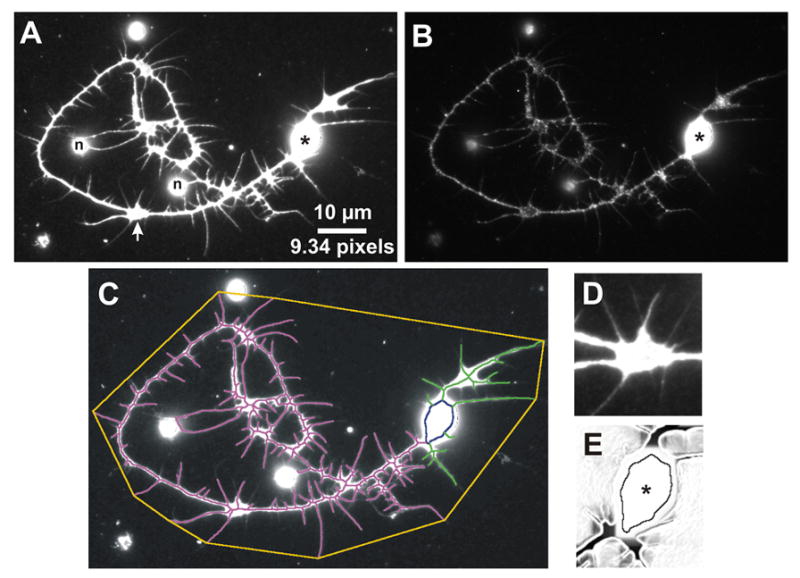
Images of a fluorescently labeled neuron and graphic representations of the output generated by NeuronMetrics. (A, B) Double-labeled images of a cultured neuron. (A) Anti-HRP labels all neuronal membranes with uniform, high signal intensity, which is optimal for accurate skeletonization. Even the broad neurite region (marked with arrow; enlarged in panel D) shows uniform signal intensity. This is an ideal input image for NeuronMetrics. The dark pixels on the right side of the cell body are an artifact resulting from overexposure during image acquisition. Asterisk, cell body; n, noise enclosed by neurites. (B) Anti-GreekBetagal immunostaining identifies this neuron as a mushroom body GreekGamma neuron but the signal intensity is too low and patchy for optimal skeletonization by NeuronMetrics. (C) Graphic output of NeuronMetrics computation. The neurite skeleton (dominant primary neurite in magenta, remainder in green) provides an excellent representation of neuronal morphology. The cell body region of interest (ROI) is indicated in dark blue and the neuron territory is bounded by the orange polygon. The skeleton, cell body ROI, and polygon have been thickened to 3 pixels to improve visualization. (D) Enlargement of the broad neurite region in (A), showing uniform, high signal intensity throughout. (E) Cell body region after Sobel edge detection and rolling-ball background subtraction, showing the computed cell body ROI.

A schematic overview of NeuronMetrics’ image processing steps is shown in Fig. 2. The main modules are Setup, Neuron & Cell Body, Skeletonize & Improve, Length Correction (optional), Dominant Neurite (optional), and Measure Skeleton. In Setup, a dialog box is used to indicate the location of the input images, their scale, which skeletonization mode to use for the input image set (see section 2.3), and the optional steps to be performed. Processing begins with the Neuron & Cell Body module which runs a suite of four modules. Neuron ROI, Noise ROIs, and Click Cell Body run sequentially on each displayed neuron image allowing the user to circle the neuron of interest, circle noise to eliminate it (optional), and click to indicate the location of the cell body. Afterwards, the folder of images is automatically run through Cell Body ROI (details in section 2.2). The user runs the Skeletonize & Improve module (details in section 2.3) to skeletonize the neuron (Skeletonize Neuron), fill gaps in the skeleton and remove disconnected noise (Improve Skeleton). The skeletonization steps are fully automated for the whole folder, unless the user has chosen individual handling (during Setup) because of signal variation among the images. In this case, the module pauses with each image displayed and prompts the user to indicate which of two alternative skeletonization modes to use. If the neuron contains regions of self-fasciculation, the Length Correction module may be run, and if the PI is to be computed, the Dominant Neurite module is used to isolate the dominant primary neurite (details in sections 2.5.2 and 2.5.3, respectively). Last, the Measure Skeleton module is run to automatically compute all morphometric parameters, including territory with the Polygon module.

Fig. 2.

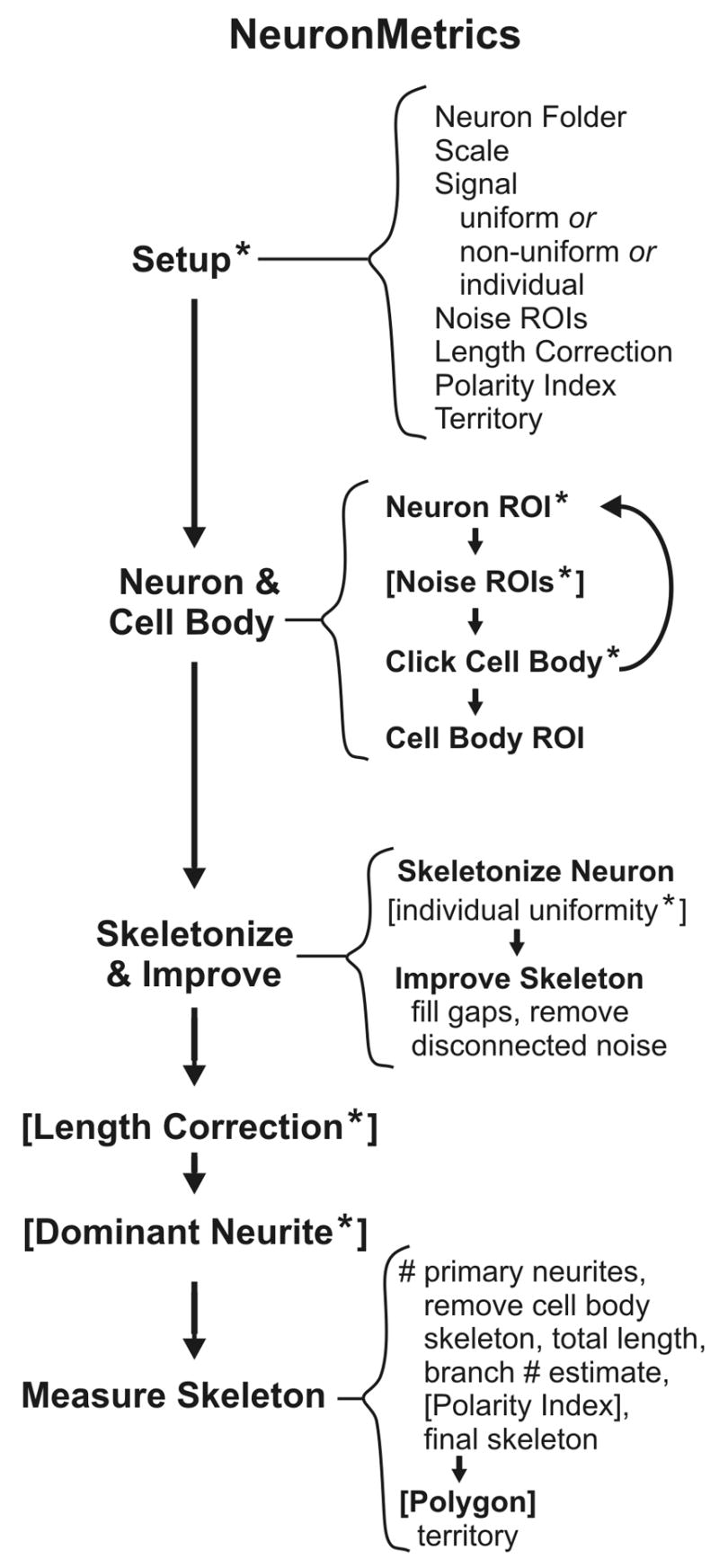
Schematic overview of the processing steps in NeuronMetrics. Square brackets indicate optional steps and asterisks indicate steps that require user input. Main modules (bold text along left side) are run by selecting them under the ImageJ “Plugins” [sic] menu. When processing a batch of images with the Neuron & Cell Body module, Neuron ROI, Noise ROIs, and Click Cell Body run sequentially on each image in the folder because the user performs a brief manual task in each step. Subsequently, all images in the folder are automatically run through Cell Body ROI. Thereafter, the user initiates the desired module, in sequence, to process all images in the folder in batch mode.

To expedite processing of a batch of neuron images from a selected input folder, input files are automatically opened, processed through automated steps, and closed. Output files and folders are automatically created, named, and saved. If the module includes manual intervention, the tool that will be used is pre-selected, and the user proceeds to the next step by pressing the space bar or clicking a button. These features greatly reduce the time spent on file management and maneuvering about the graphical interface. Images (e.g., skeletons) are automatically saved, optionally superimposed on the neuron image, so that their accuracy can be verified by visual inspection.

2.2. Cell Body ROI module

An approximate representation of the cell body perimeter is needed to establish the base of primary neurites and to exclude the cell body skeleton from the neurite length computation. NeuronMetrics semi-automatically generates a cell body ROI (Fig. 1E) by creating an image in which most of the cell body has a single gray value and then finding the perimeter of that uniform region. It uses ImageJ’s edge-finding algorithm (a Sobel edge detector) and background-subtraction algorithm (URL list, background) to set the central cell body pixels to a single gray value (Supplement 1: Rolling Ball Radius). The cell body ROI is then created using the user-provided cell body location and ImageJ’s wand tool to find the perimeter of the region with uniform pixel value. Success of this approach depends on the signal in the cell body region being saturated as happens during the relatively long exposures needed to image fine neurites.

2.3. Skeletonize & Improve module

The skeletonization approach is depicted in Fig. 3. The neuron image (Fig. 3A) is preprocessed with an empirically determined sequence of image-processing methods with empirically determined parameters (Supplements 1, 2). The preprocessed image is used to create both the Thresholded image, showing the major neurites and broad regions such as the cell body and branch points (Fig. 3B), and the Laplacian image, with enhanced representation of fine neurites (Fig. 3C). Next, these two images are merged and this Merged image (Fig. 3D) is skeletonized to yield a Preliminary Skeleton (Fig. 3E). The Preliminary Skeleton is one-pixel wide except at some branch points and may contain noise and a few gaps, resulting from localized spots of low-intensity signal. The Final Skeleton is created by filling gaps, eliminating disconnected noise, removing the cell body skeleton, and removing any primary neurites below a threshold length, to generate a fully-connected skeleton that represents the complete neurite arbor (Fig. 3F).

Fig. 3.

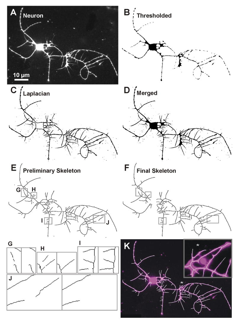
Skeletonization steps performed by NeuronMetrics. (A) Fluorescent anti-HRP image of a cultured neuron. (B, C) Two images created after pre-processing. (B) Thresholded image detects the high intensity fluorescent signal. (C) Image created using Laplacian edge detection enhances fine neurites. (D) Merged image created by combining the black regions of the thresholded and Laplacian images. (E) Preliminary skeleton generated by skeletonizing the merged image. Boxed regions have gaps in the skeleton or disconnected noise. (F) Final skeleton generated after gaps are filled, disconnected noise is removed, and the cell body skeleton is cleared. (G–J) Enlargements of boxed regions in (E) and (F), showing gaps and noise in the preliminary skeleton (left panels) and the outcome of gap filling and noise removal in the final skeleton (right panels). (K) Final skeleton (white) superimposed on a false-colored neuron (magenta). The inset is an enlargement of the region marked by the asterisk, showing the one-pixel-wide skeleton and a spot of enclosed noise that was manually excluded using the optional Noise ROIs module. The skeletons in E, F, and the main panel of K were thickened to three pixels to improve visualization.

Gaps in the preliminary skeleton are filled by finding pairs of endpoints on the skeleton that are near one another and then filling the gap if the two skeleton sections lie sufficiently close to a line drawn between the endpoints (Fig. 4). The gap-filling algorithm assumes the skeleton can be approximated by a straight line over short distances and is designed to be sensitive to curves near skeleton endpoints to reduce the chance of connecting noise to neurites. It uses empirically determined values for gap distance, extend distance, and maximum deviation (Supplement 1: Gap Filling). The algorithm is as follows: Given point p at the end of curve c₁, a portion of a skeletonized neurite, and point q at the end of curve c₂ where the distance between p and q is less than or equal to the gap distance (Fig. 4A,C), draw a line segment between p and q (Fig. 4B,D; solid red) and then extend the line segment by the extend distance at each end (dashed red). The new extended line segment endpoints are p' and q'. If the distance between the line segment extensions and the nearby curves is less than the maximum deviation, then c₁ and c₂ are considered to be a bona fide gap endpoints in the neurite skeleton and the gap is filled. To determine if the curve is close enough to the extended line segment, we traverse back on curve c₁ from p for extend distance number of pixels. At each curve c₁ pixel, if there is a pixel on the segment extension (p, p') located at a distance less than or equal to the maximum deviation, the curve is sufficiently close to the line segment. If any pixel on the curve fails this 'close to' test, the gap (p, q) is not filled. The same is done for curve c₂ using segment extension (q, q'). The gap in Fig. 4A would be filled while the one in Fig. 4C would not.

Fig. 4.

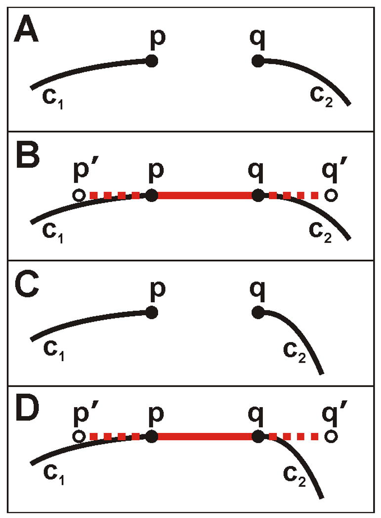
Diagramatic representation of NeuronMetric’s gap-filling method. Each panel shows two portions of curvilinear neurite skeleton, c₁ and c₂, with endpoints p and q, respectively. (A) A gap, for example within a neurite, that will be filled. (B) The solid red line segment drawn between p and q and the dashed-red extended line segment to endpoints p’ and q’. Because the distance between the line segment extensions and the nearby curves is less than some specified maximum deviation, the gap between c₁ and c₂ will be filled. (C–D) A gap, for example between two different neurites, that will not be filled because pixels on curve c₂ fail the 'close to' test.

Results from the gap-filling method are shown in Fig. 3G–J before (left panels) and after (right panels) filling gaps. In Fig. 3G a gap near the end of a neurite fails to be filled due to a noise-induced curve in the skeleton near the gap. Hence, the distal pieces of the fine neurite are lost from the skeleton. Fig. 3H shows a gap in each of two fine neurites. The lower gap is flanked by two endpoints, one on a proximal skeletonized piece of the fine neurite branching from the parent neurite and the other on the distal piece of the fine neurite. The upper gap is flanked by only one endpoint because weak signal at the branch point resulted in the skeleton having no nascent branch off the parent neurite. Because two endpoints must be present to define a gap, the lower gap is filled, but the upper gap is not. However, even a short nascent branch (Fig. 3I) is sufficient to provide an endpoint so a gap may be filled. In Fig. 3J a gap between a neurite tip and a piece of debris is not filled because the gap distance is greater than the user-defined gap distance. Because the algorithm is designed to be sensitive to curves near skeleton endpoints in order to reduce the chance of connecting noise to neurites, it probably would not have filled this gap even if the span had been shorter. The gap-filling algorithm can potentially cause closely aligned neurite tips to be connected but only occasionally connects noise to the skeleton.

After gap filling, background noise that has been skeletonized but is not connected to the neuron skeleton is eliminated by traversing the skeleton from an arbitrary pixel on the cell body skeleton (i.e., a skeleton pixel within the cell body ROI) to collect the connected pixels representing the neuron. A new image (“Improved Skeleton”) is created in which only these skeleton pixels are represented. Removal of the cell body skeleton, by clearing inside the cell body ROI with ImageJ’s “Clear”, and elimination of very small primary neurites below a designated threshold length (see section 2.4), yields the Final Skeleton image (Fig. 3F, 3K), which represents the neurite arbor with a high degree of fidelity.

A special case occurs in the images of neurons, especially from particular mutant strains, with large broad neurite regions having non-uniform signal intensity (Fig. 5; compare with Fig. 1). Such images are best processed differently when creating the thresholded image. If the user indicates that an image or set of images has non-uniform gray values (a setting in the Setup module), the preprocessed image is smoothed twice followed by thresholding using ImageJ’s thresholding function (which uses an isodata algorithm; Ridler and Calvard, 1978). Figs. 5D and 5E compare the two modes of skeletonization through regions of non-uniform signal intensity.

Fig. 5.

Skeletonization of a neurite region with non-uniform fluorescent signal. (A) Anti-HRP image of a neuron with regions of broad, non-uniform signal (e.g., arrow). (B) Skeleton (red), obtained using the non-uniform signal mode, superimposed after thickening to three pixels to improve visibility. (C–E) Enlargement of a region, marked by arrow in panels A and B, which has non-uniform signal. For comparison, see Fig. 1D which shows an enlarged broad region with uniform signal. (C) Fluorescent image. (D) Overlay of the skeleton (one pixel wide) created using non-uniform signal mode, which results in the desired representation of neurite branching. (E) If uniform signal mode is used, the resulting skeleton encloses the darker gray sub-regions instead of traversing them, which would cause spurious length and branch number computations.

We determined the fidelity of the skeletons by visual inspection of >1,000 superimposed images acquired from >12 datasets representing several genotypes and two hormone-treatment conditions. The neurite arbors of these neurons span a wide range of size and complexity. For neurons having uniform fluorescent signal intensity, the skeleton provides an excellent representation of the neuron (Figs. 1C, 3K), although, if present, regions of self-fasciculation require manual and automated corrections for accurate length and branch counts, respectively (see sections 2.4.2 and 2.5.2). For neurons having non-uniform fluorescent signal, skeletonization using the non-uniform mode also yields excellent skeletons (Fig. 5). However, because the non-uniform mode does not represent self-fasciculated regions well, for neurons with both non-uniform signal and self-fasciculation (a relatively rare occurrence among wild-type neurons), the user must decide which feature to optimize. Final skeletons generated by NeuronMetrics were suitable as input to the automated neurite-curvature computation (K. Barnard, R. Kraft, M. Escobar, M. Narro and L. Restifo, unpublished) that had been developed for use with manually edited, precise skeletons (Kraft et al., 2006).

Analysis of subtle errors revealed that NeuronMetrics may fail to skeletonize some fine terminal neurites and incorrectly skeletonizes some small noise as short neurites; these errors have opposite effects on branch count and may cancel each other out over an entire data set. Programming efforts to reduce these errors introduced as many as were eliminated. The final skeleton may still have features that confound branch number determination. We followed a strategy of analyzing the confounding features and adjusting the quantitative measurements accordingly (see section 2.4.2).

If indicated, two optional processing steps may be performed prior to using the skeleton to measure morphometric parameters. Length correction may be performed on neurons having significant regions of self-fasciculation (see section 2.5.2). If the PI computation is desired, the dominant primary neurite is isolated (see section 2.5.3).

2.4. Measure Skeleton module

2.4.1. Neurite arbor length

Total neurite length is computed by traversing the final skeleton from each primary neurite’s base pixel (see section 2.4.3), assigning horizontal or vertical steps a value of one and diagonal steps a value of SquareRoot2. The total length is the sum of the values of all steps plus, if needed, a length correction for regions of self-fasciculation (see section 2.5.2). This total is converted to length units using the scale of the image. Computing length by this method is widely accepted because it measures the length of the polygonal path connecting the pixel centers on the skeleton. Hence, because the skeletons represent the neuron images well, the length measurements have a high degree of accuracy (see section 2.6).

2.4.2. Branch number estimate

In vivo, neurites are branched structures with branch points of degree three (three paths lead out) and branch tips (endpoints) of degree one. As a consequence, the number of branch points equals the number of branch tips minus one, which intuitively follows from the fact that each branch has a beginning and an end, and which can formally be proved by induction. If the neurites of a cultured neuron did not contact one another, the branch number could be determined directly from the skeletonized image by counting either branch points or endpoints. However, in vitro, the neurites frequently contact one another, forming false branch points and often obscuring endpoints. In practice, counting endpoints in the neurite skeleton is more straightforward than counting branch points because an un-obscured neurite tip is reliably skeletonized as a degree one pixel. Thus, there is a 1:1 correspondence between an obscured tip in the neurite image and the absence of a degree one pixel in the skeleton. In contrast, there is not a 1:1 correspondence between false branch points and degree-three pixels because a false branch point may skeletonize as one or more isolated degree-three pixels. Furthermore, in our neurons, the branch angle, formed by neurites as they leave the parent neurite, varies considerably and can exceed 90°. This means the branch angle is not useful for distinguishing between the base of a branch and a neurite contact point. Therefore, our approach for computing a reasonable branch number estimate is to count endpoints, and account for those obscured by neurite contacts.

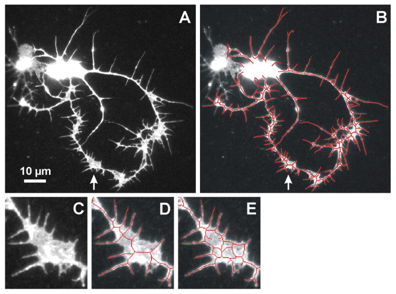
To address this challenge, we developed a method for adjusting the branch number estimate using features called faces in computational geometry. When neurites contact one another, the resulting skeleton partitions the image into faces, where each face is a maximally connected set of non-skeleton pixels (Fig. 6B, 6E–F). In other words, one cannot move on the image from one face to another without crossing the skeleton. A face is unbounded by the skeleton if it contains pixels on the boundary of the image; otherwise the face is bounded. Faces are relevant to the branch number estimate because, for example, when a neurite tip touches another neurite, an endpoint is obscured, a false branch point is created, and a face is created (Fig. 6A–B, see “t”). For each such face, we desire that the endpoint count be increased by one. Tip-to-neurite is the most common case of simple contacts that give rise to faces.

Fig. 6.

Detection and assessment of faces in neurite skeletons for use in the branch-count correction. (A) A cultured neuron demonstrating three types of simple neurite contacts: t, tip-to-neurite; d, tip-to-tip; x, neurite crossover. (B) Neurite skeleton depicting all faces resulting from neurite contacts. The unbounded face is beige and bounded faces are other colors. The tip-to-neurite contact at t causes the light green face; the tip-to-tip contact at d causes the lavender face; and the crossover at x causes the red face. (C) Enlargement of a self-fasciculating region of a cultured neuron. Note that the distance between adjacent neurites varies, resulting in periodic contacts in the neurite skeleton. (D) View of the whole neuron. (E–F) Corresponding neurite skeletons with each face a different color. Faces are labeled based on their classification by size and shape: s, small; m, medium; e, elongated medium; L, large. (E) Enlarged view of faces along a region of self-fasciculation. The series of adjacent small faces results from self-fasciculation rather than from tip touching. They are categorized as F₁ faces and are excluded from the branch-count correction as desired. The two elongated faces are categorized as F₂ faces and are excluded from the branch-count correction. This is the desired outcome for the purple elongated face, but not for the rose face which results from a tip-to-neurite contact. (F) View of all faces in the neuron. Note that the large faces, non-elongated medium faces, and isolated small faces often result from tip touching. Using categorized faces to correct for obscured neurite tips improves the branch count estimate: 13 of the 15 faces in panel (B) and 4 of the 12 faces in panel (F) are added to the respective endpoint counts.

Other neurite contacts to consider are tip-to-tip, crossovers, and self-fasciculation. When two neurite tips touch and form a face (Fig. 6A–B, see “d”), two endpoints have been obscured. Ideally, the endpoint count should be increased by two. Conversely, when neurites cross over each other (Fig 6A–B, see “x”), a face is formed, but the neurite tip is not obscured, so the endpoint count does not need adjustment. Because of the lack of diagnostic features for faces resulting from tip-to-tip and crossover contacts, we can not specifically correct for these categories. Tip-to-tip and crossovers, which are less common cases of simple contacts, yield complementary errors (the method under-corrects by one or over-corrects by one, respectively).

Like crossovers, regions of self-fasciculation result in faces that do not represent obscured endpoints. In fact, self-fasciculation tends to generate many faces which we would not want to add to the endpoint number (Fig. 6C–F). Fortunately, the faces created by self-fasciculation have diagnostic features: small faces adjacent to other small faces and elongated faces of medium size (Fig. 6E). Such faces are much less common outside self-fasciculating regions. Therefore, we identify them and exclude them from the branch number adjustment.

Thus, our general strategy is to find all faces using a depth-first traversal algorithm (Cormen et al., 2001; see Supplement 3 for details). Faces are categorized and all bounded faces, except the type that are common in self-fasciculating regions, are added to the endpoint count. We define a small face as having an area less than A_s, a medium face as having an area larger than a small face but smaller than A_m, and a large face as having an area larger than A_m (Fig. 6E–F). We define an elongated face as having both a medium size and a roundness less than R_e (Fig. 6E). The parameters A_s, A_m, and R_e have empirically determined values (Supplement 1, Branch Count). The roundness of a face is estimated by comparing its area/diameter ratio to that of a circle having the same diameter, where diameter is defined to be the longest distance between any two points on the object boundary. Specifically, for a face having measured values area_f and diameter_f we define

$${\text{roundness}}_{\text{f}}=({\text{area}}_{\text{f}}/{\text{diameter}}_{\text{f}})/({\text{area}}_{\text{c}}/{\text{diameter}}_{\text{f}}),$$

where subscripts f and c stand for face and circle, respectively.

We subdivide the set of bounded faces F into three empirically determined disjoint (mutually exclusive) subsets, F₁, F₂, and F₃. F₁ is the set of small faces that are adjacent to one or more other small faces. F₂ is medium-sized, elongated faces. F₃ is the set of all other bounded faces (isolated small faces, non-elongated medium faces, and all large faces), explicitly:

$${\text{F}}_3=\text{F}-{\text{F}}_1-{\text{F}}_2.$$

The number of F₃ faces is added to the endpoint count.

The number of primary neurites must be substracted because the base pixel of each is not a true endpoint. A final correction excludes very short neurites, defined to be less than 5 pixels (0.5 μm), which is within the range of noise. The equation for estimating branch number is:

$$\text{branch\hspace{0.17em}number\hspace{0.17em}estimate}=\#\text{endpoints}+{\#\text{F}}_3\hspace{0.17em}\text{faces}-\#\text{primary\hspace{0.17em}neurites}-\#\text{short\hspace{0.17em}neurites}.$$

To verify that all faces were found, we created test images from neuron skeletons in which each face found was filled with an arbitrary color (e.g., Fig. 6). Missed faces would remain white. Visual inspection of > 400 such images, derived from neuron arbors with a wide range of sizes and shapes, indicates that all faces are found.

To determine the validity of branch number estimates computed by NeuronMetrics, we manually analyzed a set of 59 neurons from a single typical experiment. Note that manual branch counts require applying human judgment to ambiguities that arise due to neurite-arbor complexity. Given the constraints imposed by 2D static images, it can be difficult to state the true branch number for a given neuron. With this caveat, our expectation is that automated branch counts should approximate manual branch counts. In the past, we compared manual branch counts (done on the original neuron images) with those obtained from manually edited SimplePCI skeletons, which also require human judgment of neuron morphology. We found that, for the great majority (88%) of neurons, the two estimates were within 20% of each other, with the SimplePCI-based values tending to be lower than those obtained by manual counting (data not shown). In the present analogous comparison on a new set of neuron images, automated branch number estimates from NeuronMetrics and manual branch counts were within 20% of each other (Fig. 7). Over most of the population, the deviations between the two values were balanced, i.e., some neurons gave higher values with manual counts and others gave higher values with NeuronMetrics. For those neurons with the largest number of branches (~10% of the population), NeuronMetrics’ branch-number estimates tended to be smaller than the manual branch counts. In summary, NeuronMetrics’ fully automated branch-number estimates are as good as the values obtained by the much slower and more laborious method based on manually edited skeletons.

Fig. 7.

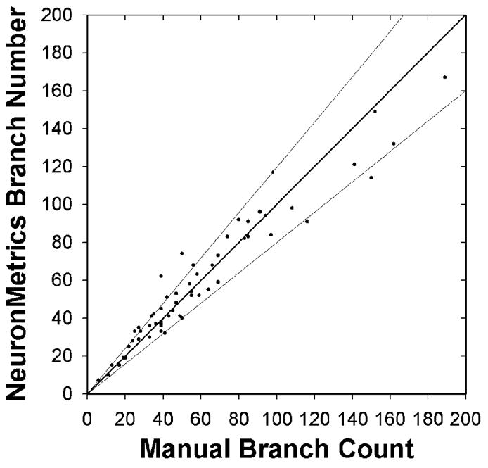
Validation of branch number estimate. Comparison of manual branch counts based on neuron images with NeuronMetrics automated branch number estimate based on skeletonized representations of the same images (n = 59 neurons from a single experimental data set). The dark line represents identical values (x = y). The majority of points fall within the thin lines which represent (+) and (−) 20%.

2.4.3. Number of Primary Neurites

We determine the number of primary neurites by locating their roots, that is, the points where they emerge from the cell body. The location of these roots can be approximated by the points where the skeleton contacts the cell body ROI (Fig. 8A,B). We find these roots by traversing each skeleton fragment inward, starting from a slightly expanded cell body ROI (Supplement 1: Primary Neurites, Expand ROI), until a pixel is found that contacts the original cell body ROI (Fig. 8B–D). That pixel is added to a list of candidate base points. After completion of the traversal, duplicate or neighboring primary neurite base points are removed from the list. A neurite must exceed an empirically determined length threshold (Supplement 1: Primary Neurites, Length) to be considered a primary neurite. Skeletonized primary neurites below the threshold are eliminated from the skeleton.

Fig. 8.

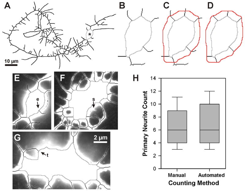
Primary neurite count. (A–D) Computing the root of each primary neurite. All or part of the skeletonized neurite arbor is shown inverted, with the cell body ROI in light gray. See Fig. 1A for original neuron image. (A) Final skeleton of neurite arbor, thickened to improve visibility. Asterisk marks the cell body. (B) Enlarged view of cell body ROI and the proximal portions of the primary neurites. (C) The expanded cell body ROI (red), as computed by NeuronMetrics and added to the image in (B). (D) NeuronMetrics has removed skeleton pixels distal to the expanded cell body ROI, leaving only the skeleton pixels that connect the two ROIs. The root of each primary neurite is found by traversing each skeleton fragment from the expanded cell body ROI to the first skeleton pixel that contacts the cell body ROI. (E–G) Assessment of primary neurite count. Three different neuron cell bodies, showing the cell body ROI (gray) and adjacent skeletonized neurites (black) superimposed on the corresponding fluorescent image. Skeleton has been eliminated from the cell body regions. The automated primary neurite counts vs. manual counts are 6 vs. 5 (E), 17 vs. 18 (F), and 11 vs. 10 (G). Errors in the automated counts, relative to human interpretation of the neuron, result from skeletonization error (see e in E) and a neurite tip touching the cell body (see t in G). In F, a very short neurite (see s), that did not meet the primary-neurite length threshold, had been counted manually. (H) Validation of primary neurite count. Comparison of manual and automated primary neurite counts performed on a set of 59 neurons (images are from the same experiment depicted in Fig. 8). Box-plot distributions with the median indicated by the line inside the box. Top and bottom of the box represent the 75^th and 25^th percentiles, respectively, and the upper and lower crossbars represent the 90^th and 10^th percentiles, respectively. The median values are identical and the Mann-Whitney rank sum test shows no statistically significant difference (P = 0.66).

We visually inspected >1,000 images with the cell body ROI superimposed on the corresponding neuron and found that the computed ROI delineates the cell body very well. It is contained within the cell body and every pixel of the ROI is roughly equidistant from the cell body boundary. Fig. 8E–G shows examples of primary neurite computation and some of the sources of error in the automated primary neurite count.

The primary neurite count was validated by comparing the automated count with manual counts for a set of 59 neurons from the same experiment. The median number of primary neurites was 6 for both methods (Fig. 8H). A Mann-Whitney rank-sum test showed no significant difference between the two distributions.

2.4.4. Polygon module

We define the territory of a neuron to be the area of the smallest convex polygon (i.e., convex hull) that encloses its final skeleton and cell body ROI (Fig. 9) (Kraft et al., 2006). The convex hull vertex set for a skeletonized neuron is computed using a modified Graham’s scan algorithm (Graham 1972; Andrew 1979). The vertices are connected to form a convex polygon and its area is computed using ImageJ’s Measure feature (URL list, measure). Given an accurate representation of the neuron images, such as the skeletons and cell body ROI’s generated by NeuronMetrics, Graham’s scan computes the correct convex polygons. Indeed, visual inspection of >1,000 images with the polygon superimposed on the neuron confirmed the accuracy of the territory computation.

Fig. 9.

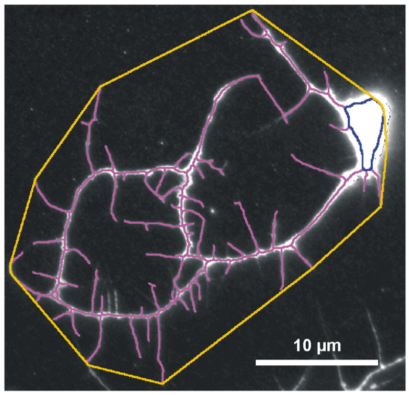
Fluorescent anti-HRP image of a cultured neuron, with superimposed neurite skeleton (magenta) and cell body ROI (dark blue). The territory (orange) of the neuron, computed by NeuronMetrics, is the area of the smallest convex polygon that encloses the skeleton and cell body ROI. The skeleton, cell body ROI, and polygon have been thickened to 3 pixels to improve visualization. This random neuron is from a wild-type (OreR-C) culture prepared from the central brain region of a larval CNS.

2.5 Optional Manual Steps

2.5.1. Noise ROIs module

If necessary, noise enclosed by neurites may be removed after circling it using the Noise ROIs (Fig. 2; 3K).

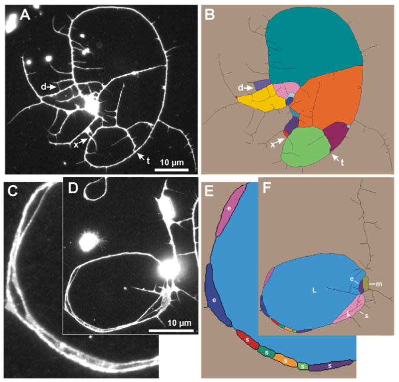
2.5.2. Length Correction module

Computing a reasonably accurate length estimate from images of cultured neurons is challenging for neurons that self-fasciculate (Fig. 10). Regions of self-fasciculation confound the length computation because multiple (2–4) adjacent, tightly-bundled neurite sections are skeletonized as a single neurite (Fig. 10A,B). The Length Correction module facilitates manual tracing and weighting of self-fasciculating neurites by allowing a user to toggle between views of the neuron with and without superimposition of the skeleton. The corrected length is:

Fig. 10.

Example of a cultured neuron with extensive self-fasciculation which necessitates length correction. (A) Fluorescent anti-HRP image of the neuron. (B) Improved neurite skeleton at same scale as in A (note that the cell body skeleton is present). (C–D) Enlargements of two regions of self-fasciculation from the areas indicated in A. (C) A bundle of three strands runs clockwise; at the arrow, one strand breaks away while the other two remain very close. (D) Three adjacent strands.

$${\text{length}}_{\text{corr}}={\text{length}}_{\text{init}}+(\text{traced\hspace{0.17em}}{\text{length}}_1\times {\text{weight}}_1)+\dots +(\text{traced\hspace{0.17em}}{\text{length}}_{\text{n}}\times {\text{weight}}_{\text{n}}).$$

The use of a weight allows the user to trace a long region of self-fasciculation, parts of which have different numbers of adjacent bundled neurites skeletonized to varying degrees of accuracy, instead of having to trace numerous short regions individually. For example, the neuron in Fig. 10A has a long self-fasciculating neurite that makes approximately 2.5 loops around a circular region. Much of the skeleton shows only a single neurite (Fig. 10B). To correct the length, the user quickly traces the entire circular region and assigns a weight of 1.5 to increase the total neurite length by 1.5 times the perimeter of the circular self-fasciculating region. The traced object remains associated with the skeleton so the length correction is taken into account if the user chooses to determine the PI (see below).

2.5.3. Dominant Neurite module

Kraft et al. (1998) defined the PI as the maximum percentage of total neurite length contributed by a primary neurite and all of its branches. The dominant neurite is the primary neurite arbor with the maximum length. In order to compute the PI, the dominant primary neurite must be isolated in the skeleton, i.e., contacts with other primary neurites must be disconnected, and its length computed. We developed the Dominant Neurite module to facilitate manual isolation of the dominant neurite without tedious pixel-by-pixel editing of skeletons (Fig. 11). The user isolates the neurite by clicking near the skeleton to indicate locations where neurites make contact and the skeleton needs to be disconnected. Although the identity of the dominant neurite is often obvious, multiple candidates may be identified if necessary. Three neurite contact cases are handled (Fig. 11C–E). In the first, when the tips of two neurites touch, three pixels are removed to create a visible gap, a simple break in the skeleton (Fig. 11E, arrow ‘s’). In the second case, when a neurite tip touches somewhere along another neurite, the user presses the ‘t’ key while clicking on the skeleton image to indicate that the break needs to be trimmed to eliminate a false branch point (Fig. 11E, arrow ‘t’). Trimming results in the removal of all pixels between the skeleton pixel nearest the mouse click and the nearest branch point pixel in the skeleton. In the third case, when one neurite crosses over another neurite, the user presses the ‘c’ key while clicking on both sides of the crossover on the skeleton image to temporarily break the crossover (Fig. 11E, arrow ‘c’). The break is made temporary to handle the situation in which both the upper and lower neurites in the crossover are candidates for dominant neurite. Preview buttons allow the user to verify that the editing has isolated the neurite(s) of interest. If the user indicates multiple candidates for dominant neurite, the software measures the length of each candidate to determine which is dominant. If a length correction has been made for self-fasciculation (see above), it is taken into account when determining length of the dominant neurite.

Fig. 11.

Isolating the dominant neurite for polarity index (PI) determination. (A) Fluorescent anti-HRP image of a cultured neuron in which the dominant neurite contacts other neurites. (B) Improved neurite skeleton, at the same scale as in A, with the dominant neurite colored red and cell body skeleton automatically removed. The skeleton has been thickened to 3 pixels to improve visualization. (C–E) Enlargements of the boxed region of A. (C) Fluorescent image. Arrows indicate tip-tip contact (s), tip-neurite contact (t), and a neurite crossover (x). (D) Neurite skeleton overlaid on the fluorescent image before isolating the dominant neurite. (E) Skeleton overlay after isolation of the dominant neurite, which is shown in red. Arrows indicate how the dominant neurite was isolated: s, simple break; t, trimmed break; x, temporary (hence no longer present) break.

2.6. Speed and quality of NeuronMetrics output

Four independent users (graduate and undergraduate students) participated in testing NeuronMetrics and validating its output. The software was run on standard desktop computers (2.8–3.0 GHz Pentium® 4 processor; 1GB RAM) or laptop computer (1.86 GHz Pentium® M processor; 512 MB RAM) using the Windows XP operating system. Individual images were 1.3MB (1344 x 1024 pixels) in size and pixel depth was 8 bits. Using NeuronMetrics, a typical set of approximately 60 images needing minimal manual intervention (i.e., no length correction or dominant neurite isolation) can be batch-processed in about an hour. For a data set requiring many optional manual steps, processing may take an additional 60–90 minutes. These data-processing times refer not to algorithm run times, but rather to the interval between selecting a folder of images and obtaining a table of numeric data. Thus, the speed of data acquisition is 1–2½ minutes per neuron. In our previous computer-assisted manual analysis, simple neurons took 25–30 min, while large, complex neurons could take as long as 90–100 min. Thus, NeuronMetrics gives us an approximately 30-to-50-fold increase in speed. In addition, there are two intervals, during the batch-mode operations of the Skeletonize & Improve module (~5 min for ~60 images) and the Measure Skeleton module (~15 min for ~60 images), in which the user may leave the room.

To determine if the data output by NeuronMetrics were comparable to data generated by skeletonization with SimplePCI and manual editing (Kraft et al., 2006), we re-analyzed a set of 50 images. (Territory had not been previously determined on this particular data set and therefore could not be included in the comparison.) The older data set consisted of neurons plated at higher densities than we now use, and images had been acquired using a less sensitive camera which often resulted in higher background (Fig. 12A,B). The NeuronMetrics data have slightly higher length values than those from our previous method (Fig. 12C). This likely results from skeletonized background noise in contact with the true neurite skeleton (Fig. 12B) and neurites from neighboring neurons that would previously have been removed by manual editing. Even with these less-than-optimal images, we found no statistically significant differences in total neurite length or branch number, and the PI profiles are very similar (Fig. 12C–E). Therefore, NeuronMetrics greatly increased data analysis speed over that of our previous method, with no significant reduction in accuracy.

Fig. 12.

Comparison of data obtained using NeuronMetrics and previous SimplePCI-based image-analysis method. (A) Portion of a cultured anti-HRP-stained neuron imaged with the SpotRT camera. Background is higher than in other images in this report which were acquired with a more sensitive camera. (B) Skeleton generated by NeuronMetrics provides a good representation of the neurites, although some noise is skeletonized (asterisks). The skeleton has been thickened to three-pixels-wide to improve visibility. (C–E) Quantitative morphometric data obtained using a set of neurons from a single experiment, all imaged with the SpotRT camera (n = 50). Comparison of semi-automated NeuronMetrics method with the SimplePCI-based method that required extensive manual editing. (C, D) Pairs of box-plot distributions, with the Mann-Whitney rank sum test showing no statistically significant differences between results obtained by the two methods. (C) Total neurite length (P = 0.12). (D) Branch number (P = 0.70). (E) The PI profiles obtained with the two methods were very similar. This is the typical skewed PI profile of 201Y-marked mushroom body GreekGamma neurons.

2.7. Software availability

NeuronMetrics will be available for download, along with a detailed user manual, at iBridge™ (http://www.ibridgenetwork.org/arizona), a Kauffman Foundation-sponsored website for dissemination of academic research.

3. Discussion

3.1. Features of NeuronMetrics software

We developed modular semi-automated software that provides quantitative morphological analysis of static 2D images of fluorescent cultured neurons. It processes 8- or 16-bit gray-scale images, runs in batch mode and creates a skeletonized representation of each neuron free of gaps and noise. From the skeleton it computes size and shape parameters: total neurite length, branch number estimate, primary neurite number, and territory are automatically computed; Polarity Index (PI) requires additional user input. Numeric data are output to a tab-delimited text file for analysis with other software applications, e.g., for statistical tests. Images of the skeleton, dominant primary neurite, cell body ROI, and territory are automatically saved as TIFF files that may be superimposed on the original neuron image, providing a means for accuracy assessment and visual display. Optional features allow the user to manually remove noise, correct length in self-fasciculating regions, isolate the dominant primary neurite, or change the skeletonization mode for neurons with non-uniform signal.

Using NeuronMetrics, we are able to process a batch of ~60 single-neuron images in 1 - 2½ hours, from a folder of images to a table of numeric data. For neurons with simple morphology, processing averages one minute per image. At the other end of the spectrum, if images are noisy, neurites self-fasciculate, and the dominant primary neurite makes numerous contacts with other neurites, the additional manual effort required may increase the average processing time to 2½ minutes per image. Hence, the throughput is sufficient to analyze hundreds of images per day even when neuron morphology is complex. This speed of operation in a single, publicly available program that is easy to learn makes NeuronMetrics a useful screening tool for basic and applied research.

As discussed below, branch number, in combination with other parameters, is essential to understanding how a neuron allocates outgrowth energy to generate a mature neurite arbor. NeuronMetrics uses a novel approach to estimate branch number: it counts neurite tips (branch endpoints) and adjusts the count based on classification of faces in the skeletonized image. This is the first report of an automated branch number computation for 2D neuronal arbors that includes a correction for neurite-neurite contacts of the types that are common in cultured dissociated neurons. Further improvement would result from being able to identify two minority classes of contacts, tip-to-tip and crossovers. This will likely require a different strategy than classifying faces in skeletons, perhaps through use of Z-axis information that would reveal whether one neurite lies above another it is contacting or use of a time-series of images.

NeuronMetrics’ gap-filling algorithm has the advantage of spanning relatively wide gaps in the skeleton. The common approach, of dilating and eroding the binary image created after thresholding, is inherently limited to filling gaps of a few pixels (Sonka et al., 1999; Forsyth and Ponce, 2003). In contrast, the algorithm we developed does not limit the gap distance that can be filled. However, as the allowable gap distance increases, so does the risk of making erroneous connections. In practice, our empirically determined maximum gap distance of 15 pixels (1.4 microns; Supplement 1) fills almost all real gaps and only occasionally spans false gaps in our neuron images. The reliability of the gap-filling algorithm could be increased further by taking into consideration the trajectory of the neurite over a longer distance.

A special challenge for any neuron analysis method is presented by regions of neurite self-fasciculation. This phenomenon is uncommon in cultured neurons in general, but appears in the axonal neurites of a considerable minority of Drosophila mushroom body GreekGamma neurons harvested from developing brains. Their in vitro propensity to self-associate may be related to their expressing cell adhesion molecules that normally promote in vivo fasciculation of neighboring axons into dense parallel bundles (Kurusu et al., 2002). The optional length-correction feature in NeuronMetrics is our first attempt to compensate for the problematic skeletonization of self-fasciculated regions. It requires manual intervention and the correction value assigned is user-dependent. As a goal for future software development, one would hope to identify self-fasciculation-associated features of the neuron image or its skeleton with sufficient diagnostic sensitivity and specificity to be incorporated into an automated correction strategy. Like the challenge of neurite contacts, self-fasciculation may benefit from application of methods developed for 3D reconstruction of neurons from image stacks (Al-Kofahi et al., 2002; He et al., 2003; Schmitt et al., 2004; Brown et al., 2005; Wearne et al., 2005) and/or time series of 2D images (Al-Kofahi et al., 2006).

3.2. Requirements of NeuronMetrics

Optimal neurite-arbor skeletonization and computation of the cell body ROI by NeuronMetrics depend on a strong and relatively uniform fluorescent signal throughout all parts of the neuron. This, in turn, requires either high-level expression of an endogenous fluorescent marker, e.g., Green Fluorescent Protein (Lippincott-Schwartz and Patterson, 2003), or an abundant antigen that can be detected by immunofluorescent staining such as the Nervana membrane glycoprotein of Drosophila neurons that is detected by anti-HRP reagents (Sun and Salvaterra, 1995). Because immunolabeling and GFP-type markers are increasingly common in cellular neurobiology studies, we anticipate NeuronMetrics could have broad applicability. However, markers with low signal:noise ratios or very patchy distributions would cause numerous gaps in the preliminary skeleton, increasing the risk of loss of genuine neurites from the final skeleton. Even with our anti-HRP immunostaining method, visualization of fine terminal neurites (where the signal is weakest) requires careful focusing and image-acquisition settings that overexpose the cell body and other regions with very strong signal. This optimizes fine-neurite representation and minimizes unfilled gaps in the skeleton. However, the cost is some loss of resolution in the vicinity of the cell body and in areas of self-fasciculation. The trade-off works well for neurons with an extensive arbor away from the cell body, numerous fine terminal neurites, and infrequent self-fasciculation.

NeuronMetrics can process images with non-uniform fluorescent signal by using empirically determined image-processing parameters that allow good skeletonization (Fig. 5). This works well for neurons without self-fasciculation. Beyond this case, we have not systematically tested NeuronMetrics with less optimal labeling methods. We note, however, that it did very well in handling ‘noisy’ images (i.e., high background; Fig. 12) acquired with a relatively low-sensitivity camera. It is possible that information in the genetic-marker image (that identifies specific neuronal subsets), combined with the pan-neuronal membrane-labeled image, could help in the analysis of neurons with both self-fasciulation and non-uniform signal.

3.3. Relationship of NeuronMetrics to other image-analysis software

While developing NeuronMetrics, our emphasis was on developing a set of user-friendly tools. NeuronMetrics is complementary to other approaches that have been developed for quantitative analysis of neuron size and shape. Like NeuronMetrics, NeuronJ is a module for use with ImageJ (Meijering et al., 2004). It implements a ridge-finding algorithm based on live-wire segmentation that permits semi-automated centerline tracing of 2D fluorescent neuron images. Because the user designates the start and end of individual neurites, ambiguities due to neurite-contacts are resolved by user judgments. The outcome is excellent accuracy for individual neurites and whole neurite arbors. However, because user intervention is required at least twice to trace each neurite, it would be quite difficult for a single user to analyze hundreds of large, complex neurons per day.

Rapid, fully automated neuron tracing methods have been developed by Roysam and Turner and their colleagues, building on algorithms they devised for 2D fluorescein angiograms of retinal vasculature (Can et al., 1999). Their approach is based on exploratory vectorial tracking algorithms that start from seed points and locally trace vessel branches in a recursive manner (Kirbas and Quek, 2004). This local image analysis approach focuses only on pixels likely to contain relevant information, in order to be able to process video images in real-time (Can et al., 1999; Shen et al., 2001). In contrast, our approach uses global image processing techniques for the initial skeletonization, and then applies local exploratory methods such as gap detection and depth-first traversal. Combining global with local strategies has the advantage of not disqualifying possibly relevant pixels too early in the skeleton construction process. NeuronJ also has a global preprocessing step, which then is followed by the exploratory semi-automated tracing algorithm.

To enable automated analysis of images with a wide range of technical and biological variation, Can et al. (1999) developed exploratory algorithms that make use of localized contrast and edge gradients. From the resulting trace of the vascular tree, rapidly extracted branchpoints and crossovers (which are not distinguished from each other) serve as landmarks for alignment (registration) of repeated images of the same eye (Shen et al., 2001). Due to their geometric similarities, algorithms developed for retinal vasculature were readily adapted for fully automated tracing of neurite arbors (Al-Kofahi et al., 2002, 2003). The methods were applied to images of immunostained neurons to study the effects of surface topography on neurite outgrowth (Dowell-Mefsin et al., 2004). A recent extension of this strategy, for use with sequential images, integrates information from neurite tracing, pair-wise image registration and a binary change mask in order to interpret, via Bayesian model selection, the nature of changes over time (Al-Kofahi et al., 2006). This automated analysis method was tested on live, unstained neurons imaged with phase-contrast optics, but could likely be applied to fluorescent images of GFP-expressing live neurons. A particularly valuable feature of their change analysis is the detection of branching events (“new” or “split”) and neurite contacts (“merge”) (Al-Kofahi et al., 2006). Such a time-series approach resolves many ambiguities related to branch number, and allows accurate determination of branch-formation rates.

3.4. Utility and significance of NeuronMetrics for neuroscience

The efficiency and scope of neuroscience studies based on primary cell culture will be enhanced by readily available semi-automated morphometric tools. NeuronMetrics offers a substantial menu of morphometric features, including territory and Polarity Index. It permits fast enough image analysis that neuron sampling and image-acquisition by standard, manual microscopy methods now become the rate-limiting steps. NeuronMetrics modules run in ImageJ, which has a user-friendly interface and web-accessible supporting documentation (URL list, documentation), including a cell biology-oriented manual (URL list, manual) developed at Toronto Western Research Institute. NeuronMetrics’ also has a detailed user manual that provides illustrated, step-by-step instructions for training new users. These attributes should make NeuronMetrics attractive to many laboratories.

The availability of shape information for neurite arbors is of particular importance for classifying neuron types and for recognizing effects of physiological signaling molecules, pharmacological agents, or genetic mutations. With three of NeuronMetrics’ primary parameters (length, branch number, and territory), one can readily calculate relationships that describe the shape of the arbor. First, the ratio of branch number estimate to total length, which is highly regulated for some cultured neurons (Kraft et al., 1998), indicates the balance between extension and branching modes of neurite outgrowth. Second, territory allows assessment of neurite arbor compactness with two measures: branch density (branch number estimate DividedBy territory) and neuron sprawl (territory DividedBy total length). Mutant neurons that appear ‘small’ because of reduced territory may in fact have normal length, but distribute their neurites more compactly because of a heightened tendency to branch or because of increased neurite curvature (Kraft et al., 2006). Recognizing these distinctions is important for determining the molecular mechanisms underlying neurite arbor differences caused by genetic mutations or pharmacological treatment. PI is a powerful optional tool for evaluating the axon:dendrite balance within arbors of some cultured neurons (Kraft et al., 1998; Jacobson et al., 2006). Shifts in the PI profile of a population of neurons (Kraft et al., 2006) could indicate differential effects of mutations or exogenous agents on axons and dendrites, as has been seen in vivo (Lee et al., 2000; Arimura and Kalbuchi, 2005).

Beyond its value for individual cultured neurons, NeuronMetrics could be used to analyze neurons in vivo that have the fortuitous geometry of relatively planar arborizations, provided they are well-isolated and can be labeled a strong signal. For example, GFP-expressing dendrites of sensory neurons on the Drosophila body wall (Gao et al., 1999) appear to have such suitable features. In addition, NeuronMetrics may be able to process images of Golgi-stained neurons, such as cortical pyramidal neurons whose dendritic arborizations are relatively flat and often assessed by Sholl analysis applied to 2D photomicrographs (e.g., Kishi and Macklis, 2004; Wu et al., 2004). In fact, the PI feature of NeuronMetrics could be adapted to quantify differences between apical and basal dendritic arbors.

High-speed, fully automated tracing algorithms allow real-time, high-resolution imaging of retinal vessels for computer-assisted laser surgery (Can et al., 1999; Shen et al., 2001). While not appropriate for such demanding applications, NeuronMetrics may be suitable for more routine image analysis of retinal vasculature, e.g., to document and follow disease severity and to monitor responses to therapeutic interventions. The potential value is high because retinal vasculature is disrupted in numerous disease states and may be a marker for cerebrovascular disease (Patton et al., 2005). An “Advanced Setup” feature of NeuronMetrics allows adjustment of parameters that we optimized for our neuron images (Supplement 1). For users so inclined, this flexibility will permit them to adjust NeuronMetrics settings for their particular image analysis goals.

Drug-discovery efforts for developmental brain disorders lag decades behind those for other serious medical conditions, such as cancer, in large part because of the lack of widely available cell-based assays amenable to quantitative analysis (Restifo, 2005). NeuronMetrics has made it feasible for us to pursue small-scale drug screening to rescue mutant neuronal phenotypes identified in vitro. To expand the scope and utility of morphometric analysis of primary cultured neurons to larger-scale projects, transition to a high-throughput mode would be required. Specifically automated image acquisition (e.g., Perlman et al., 2004; Mitchison, 2005) would be linked to fully automated image analysis (e.g., Al-Kofahi et al., 2002, 2003), carried out in batch mode. While additional automation of NeuronMetrics’ operation is a realistic goal, for some parameters, notably Polarity Index and the length correction for self-fasciculation, fully automated computation will require alternative non-skeleton-based approaches. When biologically relevant neuron morphology parameters can be obtained in a high-throughput mode, it will be possible to carry out genome-wide RNA-interference screens for mutant phenotypes and large-scale drug discovery-and-development screens.

4. Experimental Procedures

4.1. Genetics and Cell Biology

Primary cultures of Drosophila neurons from the central nervous system were prepared as previously described and cultured for 3 days in vitro in the presence or absence of 20-hydroxyecdysone (Kraft et al., 1998). Except for the neuron depicted in Fig. 10 (see legend), neurons were dissociated from the brains of young pupae (5 hrs after head eversion) with one of several different genetic backgrounds. The Gal4-UAS reporter system (Brand and Dormand, 1995) was used to identify genetically marked brain neurons. Specifically, the P[Gal4]201Y driver has high-fidelity, selective expression in mushroom body GreekGamma neurons (Yang et al., 1995; Kraft et al., 1998), which allows them to be distinguished from other brain neurons in dissociated cultures (Kraft et al., 1998). It was used to drive the lacZ reporter gene whose product, GreekBeta-galactosidase (GreekBetagal), was visualized by immunostaining. A pre-absorbed polyclonal rabbit anti-GreekBetagal antiserum (Cappel) was used at a 1:5000 dilution, and detected with a Cy3-conjugated donkey anti-rabbit antiserum (Jackson Immunoresearch) at 1:500. Membranes of all cultured neurons were simultaneously visualized (Jan and Jan, 1982; Kraft et al., 1998; Sun and Salvaterra, 1995) with a polyclonal goat anti-HRP antiserum (Sigma) used at 1:500 and detected with an Alexa Fluor® 488-conjugated donkey anti-goat antiserum (Molecular Probes) at 1:500.

4.2. Image Acquisition

Cultured neurons were examined on a Diaphot 300 inverted microscope (Nikon) with a 60X oil-immersion objective (N.A. 1.4). GreekBetagal-expressing neurons were systematically identified as previously described (Kraft et al., 1998). For each of these neurons, we acquired both the anti-HRP and the corresponding anti-GreekBetagal images. Images were acquired with a Hamamatsu digital camera (ORCA285) as 8- or 12-bit TIFF images; testing was done on the 8-bit images. Images that spanned multiple microscope fields were assembled into a mosaic with commercial software (PanaVue ImageAssembler 3). The neurons depicted in Fig. 12A,B were imaged using a SpotRT digital camera (Diagnostic Instruments) to acquire 8-bit TIFF images that were analyzed using SimplePCI (Compix) software. Image-acquisition settings (exposure time and gain) for each camera were adjusted empirically to optimize the inclusion of fine terminal neurites in the image. This resulted in overexposure in regions of high fluorescence, notably in the cell body region. Overexposure also causes occasional low-signal pixel artifacts, especially on the periphery of cell body regions (visible in Fig. 1A–C and enlarged in Fig. 8E). Images were assembled and labeled in CorelDraw v.12.

4.3. Software Implementation

NeuronMetrics is implemented as Java plug-ins for NIH’s ImageJ (URL list, ImageJ) and runs on Windows operating systems (2000 and XP). It processes 8- and 16-bit 2D gray-scale images. The plug-ins are modules that serve as a processing pipeline.

4.4. Statistical analysis

Validation tests performed for primary neurite count, total length, and branch number were analyzed using the Mann-Whitney rank sum test (SigmaStat v. 1.0 and SigmaPlot 2000 software, SYSTAT).

Abbreviations

CNS

central nervous system

GreekBetagal

GreekBeta-galactosidase

HRP

horseradish peroxidase

PI

Polarity Index

ROI

region of interest

URLs

FeatureJ (v. 1.3.0): http://www.imagescience.org/meijering/software/featurej/

© Erik Meijering (developed at BioMedical Imaging Group, Swiss Federal Institute of Technology, Lausanne, Switzerland)

ImageJ: http://rsb.info.nih.gov/ij/ (developed by W. S. Rasband, Research Services Branch, National Institute of Mental Health, Bethesda, Maryland, USA, 1997-2005.)

Documentation: http://rsb.info.nih.gov/ij/docs/index.html

Background: http://rsb.info.nih.gov/ij/docs/menus/process.html#background

Manual: http://www.uhnresearch.ca/facilities/wcif/imagej/

Measure: http://rsb.info.nih.gov/ij/docs/menus/analyze.html

Skeletonize: http://rsb.info.nih.gov/ij/developer/source/index.html

References

- Abdul-Karim MA, Roysam B, Dowell-Mesfin NM, Jeromin A, Yuksel M, Kalyanaraman S. Automatic selection of parameters for vessel/neurite segmentation algorithms. IEEE Trans Image Process. 2005;14:1338–1350. doi: 10.1109/tip.2005.852462. [DOI] [PubMed] [Google Scholar]
- Al-Kofahi KA, Lasek S, Szarowski DH, Pace CJ, Nagy G, Turner JN, Roysam B. Rapid automated three-dimensional tracing of neurons from confocal image stacks. IEEE Trans Inf Technol Biomed. 2002;6:171–87. doi: 10.1109/titb.2002.1006304. [DOI] [PubMed] [Google Scholar]
- Al-Kofahi KA, Can A, Lasek S, Szarowski DH, Dowell-Mesfin N, Shain W, Turner JN, Roysam B. Median-based robust algorithms for tracing neurons from noisy confocal microscope images. IEEE Trans Inf Technol Biomed. 2003;7:302–17. doi: 10.1109/titb.2003.816564. [DOI] [PubMed] [Google Scholar]
- Al-Kofahi O, Radke RJ, Roysam B, Banker G. Automated semantic analysis of changes in image sequences of neurons in culture. IEEE Trans Biomed Eng. 2006;53:1109–1123. doi: 10.1109/TBME.2006.873565. [DOI] [PubMed] [Google Scholar]
- Andrew AM. Another efficient algorithm for convex hulls in two dimensions. Inform Process Lett. 1979;9:216–218. [Google Scholar]
- Arimura N, Kaibuchi K. Key regulators in neuronal polarity. Neuron. 2005;48:881–884. doi: 10.1016/j.neuron.2005.11.007. [DOI] [PubMed] [Google Scholar]
- Banker G, Goslin K, editors. Culturing Nerve Cells. The MIT Press; Cambridge, MA: 1998. [Google Scholar]
- Brand AH, Dormand EL. The GAL4 system as a tool for unravelling the mysteries of the Drosophila nervous system. Curr Opin Neurobiol. 1995;5:572–578. doi: 10.1016/0959-4388(95)80061-1. [DOI] [PubMed] [Google Scholar]
- Brown KM, Donohue DE, D'Alessandro G, Ascoli GA. A cross-platform freeware tool for digital reconstruction of neuronal arborizations from image stacks. Neuroinformatics. 2005;3:343–360. doi: 10.1385/NI:3:4:343. [DOI] [PubMed] [Google Scholar]
- Can A, Shen H, Turner JN, Tanenbaum HL, Roysam B. Rapid automated tracing and feature extraction from retinal fundus images using direct exploratory algorithms. IEEE Trans Inf Technol Biomed. 1999;3:125–38. doi: 10.1109/4233.767088. [DOI] [PubMed] [Google Scholar]
- Cohen-Cory S. The developing synapse: construction and modulation of synaptic structures and circuits. Science. 2002;298:770–776. doi: 10.1126/science.1075510. [DOI] [PubMed] [Google Scholar]
- Cormen TH, Leiserson CE, Rivest RL, Stein C. Introduction to Algorithms. 2. The MIT Press; Cambridge, Massachusetts: 2001. [Google Scholar]
- de Berg M, van Kreveld M, Overmars M, Schwarzkopf O. Computational Geometry: Algorithms and Applications. 2. Springer-Verlag Berlin Heidelberg New York; New York: 2000. [Google Scholar]
- Dominguez R, Jalali C, de Lacalle S. Morphological effects of estrogen on cholinergic neurons in vitro involves activation of extracellular signal-regulated kinases. J Neurosci. 2004;24:982–990. doi: 10.1523/JNEUROSCI.2586-03.2004. [DOI] [PMC free article] [PubMed] [Google Scholar]
- Dowell-Mesfin NM, Abdul-Karim MA, Turner AM, Schanz S, Craighead HG, Roysam B, Turner JN, Shain W. Topographically modified surfaces affect orientation and growth of hippocampal neurons. J Neural Eng. 2004;1:78–90. doi: 10.1088/1741-2560/1/2/003. [DOI] [PubMed] [Google Scholar]
- Fink CC, Bayer KU, Myers JW, Ferrell JE, Jr, Schulman H, Meyer T. Selective regulation of neurite extension and synapse formation by the beta but not the alpha isoform of CaMKII. Neuron. 2003;39:283–297. doi: 10.1016/s0896-6273(03)00428-8. [DOI] [PubMed] [Google Scholar]
- Forsyth DA, Ponce J. Computer Vision: A Modern Approach. Prentice Hall; Upper Saddle River, N.J.: 2003. [Google Scholar]
- Gao FB, Brenman JE, Jan LY, Jan YN. Genes regulating dendritic outgrowth, branching, and routing in Drosophila. Genes Dev. 1999;13:2549–2561. doi: 10.1101/gad.13.19.2549. [DOI] [PMC free article] [PubMed] [Google Scholar]
- Goldberg JL. Intrinsic neuronal regulation of axon and dendrite growth. Curr Opin Neurobiol. 2004;14:551–557. doi: 10.1016/j.conb.2004.08.012. [DOI] [PubMed] [Google Scholar]
- Graham RL. An efficient algorithm for determining the convex hull of a finite planar set. Inform Process Lett. 1972:132–133. [Google Scholar]
- Grubb MS, Thompson ID. The influence of early experience on the development of sensory systems. Curr Opin Neurobiol. 2004;14:503–512. doi: 10.1016/j.conb.2004.06.006. [DOI] [PubMed] [Google Scholar]
- He W, Hamilton TA, Cohen AR, Holmes TJ, Pace C, Szarowski DH, Turner JN, Roysam B. Automated three-dimensional tracing of neurons in confocal and brightfield images. Microsc Microanal. 2003;9:296–310. doi: 10.1017/S143192760303040X. [DOI] [PubMed] [Google Scholar]
- Hynds DL, Snow DM. A semi-automated image analysis method to quantify neurite preference/axon guidance on a patterned substratum. J Neurosci Methods. 2002;121:53–64. doi: 10.1016/s0165-0270(02)00231-5. [DOI] [PubMed] [Google Scholar]
- Iwasaki K, Isaacs KR, Jacobowitz DM. Brain-derived neurotrophic factor stimulates neurite outgrowth in a calretinin-enriched neuronal culture system. Int J Dev Neurosci. 1998;16:135–145. doi: 10.1016/s0736-5748(98)00011-2. [DOI] [PubMed] [Google Scholar]
- Jacobson C, Schnapp B, Banker GA. A change in the selective translocation of the Kinesin-1 motor domain marks the initial specification of the axon. Neuron. 2006;49:797–804. doi: 10.1016/j.neuron.2006.02.005. [DOI] [PubMed] [Google Scholar]
- Jan LY, Jan YN. Antibodies to horseradish peroxidase as specific neuronal markers in Drosophila and in grasshopper embryos. Proc Natl Acad Sci. 1982;79:2700–2704. doi: 10.1073/pnas.79.8.2700. [DOI] [PMC free article] [PubMed] [Google Scholar]
- Jap Tjoen San ER, Schmidt-Michels MH, Spruijt BM, Oestreicher AB, Schotman P, Gispen WH. Quantitation of the growth-associated protein B-50/GAP-43 and neurite outgrowth in PC12 cells. J Neurosci Res. 1991;29:149–154. doi: 10.1002/jnr.490290203. [DOI] [PubMed] [Google Scholar]
- Kim YT, Wu CF. Reduced growth cone motility in cultured neurons from Drosophila memory mutants with a defective cAMP cascade. J. Neurosci. 1996;16:5593–5602. doi: 10.1523/JNEUROSCI.16-18-05593.1996. [DOI] [PMC free article] [PubMed] [Google Scholar]
- Kirbas C, Quek FKH. A review of vessel extraction techniques and algorithms. ACM Comput Surv. 2004;36:81–121. [Google Scholar]
- Kishi N, Macklis JD. MECP2 is progressively expressed in post-migratory neurons and is involved in neuronal maturation rather than cell fate decisions. Mol Cell Neurosci. 2004;27:306–321. doi: 10.1016/j.mcn.2004.07.006. [DOI] [PubMed] [Google Scholar]
- Kraft R, Levine RB, Restifo LL. The steroid hormone 20-hydroxyecdysone enhances neurite growth of Drosophila mushroom body neurons isolated during metamorphosis. J. Neurosci. 1998;18:8886–8899. doi: 10.1523/JNEUROSCI.18-21-08886.1998. [DOI] [PMC free article] [PubMed] [Google Scholar]
- Kraft R, Escobar MM, Narro ML, Kurtis JL, Efrat A, Barnard K, Restifo LL. Phenotypes of Drosophila brain neurons in primary culture reveal a role for fascin in neurite shape and trajectory. J. Neurosci. 2006;26:8734–8747. doi: 10.1523/JNEUROSCI.2106-06.2006. [DOI] [PMC free article] [PubMed] [Google Scholar]
- Kurusu M, Awasaki T, Masuda-Nakagawa LM, Kawauchi H, Ito K, Furukubo-Tokunaga K. Embryonic and larval development of the Drosophila mushroom bodies: concentric layer subdivisions and the role of fasciclin II. Development. 2002;129:409–419. doi: 10.1242/dev.129.2.409. [DOI] [PubMed] [Google Scholar]
- Lee T, Winter C, Marticke SS, Lee A, Luo L. Essential roles of Drosophila RhoA in the regulation of neuroblast proliferation and dendritic but not axonal morphogenesis. Neuron. 2000;25:307–316. doi: 10.1016/s0896-6273(00)80896-x. [DOI] [PubMed] [Google Scholar]
- Lindsley TA, Kerlin AM, Rising LJ. Time-lapse analysis of ethanol's effects on axon growth in vitro. Dev Brain Res. 2003;147:191–199. doi: 10.1016/j.devbrainres.2003.10.015. [DOI] [PubMed] [Google Scholar]
- Lippincott-Schwartz J, Patterson GH. Development and use of fluorescent protein markers in living cells. Science. 2003;300:87–91. doi: 10.1126/science.1082520. [DOI] [PubMed] [Google Scholar]
- Malgrange B, Delree P, Rigo JM, Baron H, Moonen G. Image analysis of neuritic regeneration by adult rat dorsal root ganglion neurons in culture: quantification of the neurotoxicity of anticancer agents and of its prevention by nerve growth factor or basic fibroblast growth factor but not brain-derived neurotrophic factor or neurotrophin-3. J Neurosci Methods. 1994;53:111–122. doi: 10.1016/0165-0270(94)90151-1. [DOI] [PubMed] [Google Scholar]
- Matsumoto T, Oshima K, Miyamoto A, Sakurai M, Goto M, Hayashi S. Image analysis of CNS neurotrophic factor effects on neuronal survival and neurite outgrowth. J Neurosci Methods. 1990;31:153–162. doi: 10.1016/0165-0270(90)90160-h. [DOI] [PubMed] [Google Scholar]
- Meijering E, Jacob M, Sarria JC, Steiner P, Hirling H, Unser M. Design and validation of a tool for neurite tracing and analysis in fluorescence microscopy images. Cytometry A. 2004;58:167–176. doi: 10.1002/cyto.a.20022. [DOI] [PubMed] [Google Scholar]
- Mitchison TJ. Small-molecule screening and profiling by using automated microscopy. ChemBioChem. 2005;6:33–9. doi: 10.1002/cbic.200400272. [DOI] [PubMed] [Google Scholar]
- Nassogne MC, Evrard P, Courtoy PJ. Selective neuronal toxicity of cocaine in embryonic mouse brain cocultures. Proc Natl Acad Sci U S A. 1995;92:11029–11033. doi: 10.1073/pnas.92.24.11029. [DOI] [PMC free article] [PubMed] [Google Scholar]
- Patton N, Aslam T, Macgillivray T, Pattie A, Deary IJ, Dhillon B. Retinal vascular image analysis as a potential screening tool for cerebrovascular disease: a rationale based on homology between cerebral and retinal microvasculatures. J Anat. 2005;206:319–348. doi: 10.1111/j.1469-7580.2005.00395.x. [DOI] [PMC free article] [PubMed] [Google Scholar]
- Persico AM, Di Pino G, Levitt P. Multiple receptors mediate the trophic effects of serotonin on ventroposterior thalamic neurons in vitro. Brain Res. 2006;1095:17–25. doi: 10.1016/j.brainres.2006.04.006. [DOI] [PubMed] [Google Scholar]
- Perlman ZE Slack MD, Feng Y Mitchison TJ, Wu LF Altschuler SJ. Multidimensional drug profiling by automated microscopy. Science. 2004;306:1194–8. doi: 10.1126/science.1100709. [DOI] [PubMed] [Google Scholar]
- Restifo LL. Mental retardation genes in Drosophila: New approaches to understanding and treating developmental brain disorders. Ment Retard Dev Disabil Res Rev. 2005;11:286–294. doi: 10.1002/mrdd.20083. [DOI] [PubMed] [Google Scholar]
- Ridler TW, Calvard S. Picture thresholding using an iterative selection method. IEEE Trans System Man Cybernetics SMC. 1978;8:630–632. [Google Scholar]
- Rohrbough J, O'Dowd DK, Baines RA, Broadie K. Cellular bases of behavioral plasticity: establishing and modifying synaptic circuits in the Drosophila genetic system. J Neurobiol. 2003;54:254–271. doi: 10.1002/neu.10171. [DOI] [PubMed] [Google Scholar]
- Rong J, McGuire JR, Fang ZH, Sheng G, Shin JY, Li SH, Li XJ. Regulation of intracellular trafficking of huntingtin-associated protein-1 is critical for TrkA protein levels and neurite outgrowth. J Neurosci. 2006;26:6019–6030. doi: 10.1523/JNEUROSCI.1251-06.2006. [DOI] [PMC free article] [PubMed] [Google Scholar]
- Schmitt S, Evers JF, Duch C, Scholz M, Obermayer K. New methods for the computer-assisted 3-D reconstruction of neurons from confocal image stacks. Neuroimage. 2004;23:1283–1298. doi: 10.1016/j.neuroimage.2004.06.047. [DOI] [PubMed] [Google Scholar]
- Shah A, Fischer C, Knapp CF, Sisken BF. Quantitation of neurite growth parameters in explant cultures using a new image processing program. J Neurosci Methods. 2004;136:123–131. doi: 10.1016/j.jneumeth.2004.01.010. [DOI] [PubMed] [Google Scholar]
- Shen H, Roysam B, Stewart CV, Turner JN, Tanenbaum HL. Optimal scheduling of tracing computations for real-time vascular landmark extraction from retinal fundus images. IEEE Trans Inf Technol Biomed. 2001;5:77–91. doi: 10.1109/4233.908405. [DOI] [PubMed] [Google Scholar]
- Sholl DA. Dendritic organization in the neurons of the visual and motor cortices of the cat. J Anat. 1953;87:387–406. [PMC free article] [PubMed] [Google Scholar]
- Sonka M, Hlavac V, Boyle R. Image Processing, Analysis, and Machine Vision. 2. PWS Publishing (Brooks/Cole Publishing Company); Pacific Grove, CA.: 1999. [Google Scholar]
- Steiner P, Sarria JC, Huni B, Marsault R, Catsicas S, Hirling H. Overexpression of neuronal Sec1 enhances axonal branching in hippocampal neurons. Neuroscience. 2002;113:893–905. doi: 10.1016/s0306-4522(02)00225-7. [DOI] [PubMed] [Google Scholar]
- Sun B, Salvaterra PM. Characterization of nervana, a Drosophila melanogaster neuron-specific glycoprotein antigen recognized by anti-horseradish peroxidase antibodies. J Neurochem. 1995;65:434–43. doi: 10.1046/j.1471-4159.1995.65010434.x. [DOI] [PubMed] [Google Scholar]
- Takahashi RH, Almeida CG, Kearney PF, Yu F, Lin MT, Milner TA, Gouras GK. Oligomerization of Alzheimer's beta-amyloid within processes and synapses of cultured neurons and brain. J Neurosci. 2004;24:3592–3599. doi: 10.1523/JNEUROSCI.5167-03.2004. [DOI] [PMC free article] [PubMed] [Google Scholar]
- Treubert U, Brummendorf T. Functional cooperation of beta1-integrins and members of the Ig superfamily in neurite outgrowth induction. J Neurosci. 1998;18:1795–1805. doi: 10.1523/JNEUROSCI.18-05-01795.1998. [DOI] [PMC free article] [PubMed] [Google Scholar]
- Vutskits L, Gascon E, Tassonyi E, Kiss JZ. Clinically relevant concentrations of propofol but not midazolam alter in vitro dendritic development of isolated gamma-aminobutyric acid-positive interneurons. Anesthesiology. 2005;102:970–976. doi: 10.1097/00000542-200505000-00016. [DOI] [PubMed] [Google Scholar]
- Wearne SL, Rodriguez A, Ehlenberger DB, Rocher AB, Henderson SC, Hof PR. New techniques for imaging, digitization and analysis of three-dimensional neural morphology on multiple scales. Neuroscience. 2005;136:661–680. doi: 10.1016/j.neuroscience.2005.05.053. [DOI] [PubMed] [Google Scholar]
- Weaver CM, Pinezich JD, Lindquist WB, Vazquez ME. An algorithm for neurite outgrowth reconstruction. J Neurosci Methods. 2003;124:197–205. doi: 10.1016/s0165-0270(03)00017-7. [DOI] [PubMed] [Google Scholar]
- Wu CC, Reilly JF, Young WG, Morrison JH, Bloom FE. High-throughput morphometric analysis of individual neurons. Cereb Cortex. 2004;14:543–554. doi: 10.1093/cercor/bhh016. [DOI] [PubMed] [Google Scholar]
- Yang MY, Armstrong JD, Vilinsky I, Strausfeld NJ, Kaiser K. Subdivision of the Drosophila mushroom bodies by enhancer-trap expression patterns. Neuron. 1995;15:45–54. doi: 10.1016/0896-6273(95)90063-2. [DOI] [PubMed] [Google Scholar]
Associated Data
This section collects any data citations, data availability statements, or supplementary materials included in this article.