

Abstract
Two independent replica-exchange molecular dynamics (REMD) simulations with an explicit water model were performed of the Trp-cage mini-protein. In the first REMD simulation, the replicas started from the native conformation, while in the second they started from a nonnative conformation. Initially, the first simulation yielded results qualitatively similar to those of two previously published REMD simulations: the protein appeared to be over-stabilized, with the predicted melting temperature 50–150 K higher than the experimental value of 315 K. However, as the first REMD simulation progressed, the protein unfolded at all temperatures. In our second REMD simulation, which starts from a nonnative conformation, there was no evidence of significant folding. Transitions from the unfolded to the folded state did not occur on the timescale of these simulations, despite the expected improvement in sampling of REMD over conventional molecular dynamics (MD) simulations. The combined 1.42 μs of simulation time was insufficient for REMD simulations with different starting structures to converge. Conventional MD simulations at a range of temperatures were also performed. In contrast to REMD, the conventional MD simulations provide an estimate of Tm in good agreement with experiment. Furthermore, the conventional MD is a fraction of the cost of REMD and continuous, realistic pathways of the unfolding process at atomic resolution are obtained.
Keywords: Replica exchange, molecular dynamics, protein folding, protein dynamics, Trp-cage, all-atom, explicit solvent
1. Introduction
Predicting the stabilities of native and intermediate states, folding/unfolding rates, and other thermodynamic parameters of protein folding remains an outstanding challenge. One problem is that the computational expense of using realistic all-atom representations for both the protein and solvent limit the simulation run time. As such, all-atom molecular dynamics simulations are typically limited to 10 to 100’s ns, while folding experiments track the dynamics through a few μs to ms.
One approach to this problem that has received considerable attention is replica exchange molecular dynamics (REMD) (Sugita and Okamoto 1999), mainly because of the claims of improved sampling with this method, and the ability to address the thermodynamics of folding. In REMD, ‘replicas’ of the system of interest (i.e. a protein in a water environment) are simulated at different temperature/energy levels (Sugita and Okamoto 1999). Periodically, replicas are swapped between neighboring temperature/energy levels, such that over the course of the simulation each replica explores the entire temperature/energy range (Sugita and Okamoto 1999). The rationale underlying this method is that simulating at high temperatures allows the replicas to cross free energy barriers that are traps at low temperatures (Sugita and Okamoto 1999). However, the barrier crossing rate need not dramatically increase with temperature. The temperature directly affects the bias of low energy states over high energy states. Hence, the transition rate of an enthalpic barrier may change more sharply with temperature than that of an entropic barrier.
Consider the various two-state systems shown in Figure 1, which are in contact with a heat bath. The system coordinates in Figure 1a are confined to a box in phase space: −1.5 < z <1.5, −1.5 < x <1.5, with reflective walls. They evolve within the box under the potential
Figure 1. Transition rates for two-state systems with different barriers.
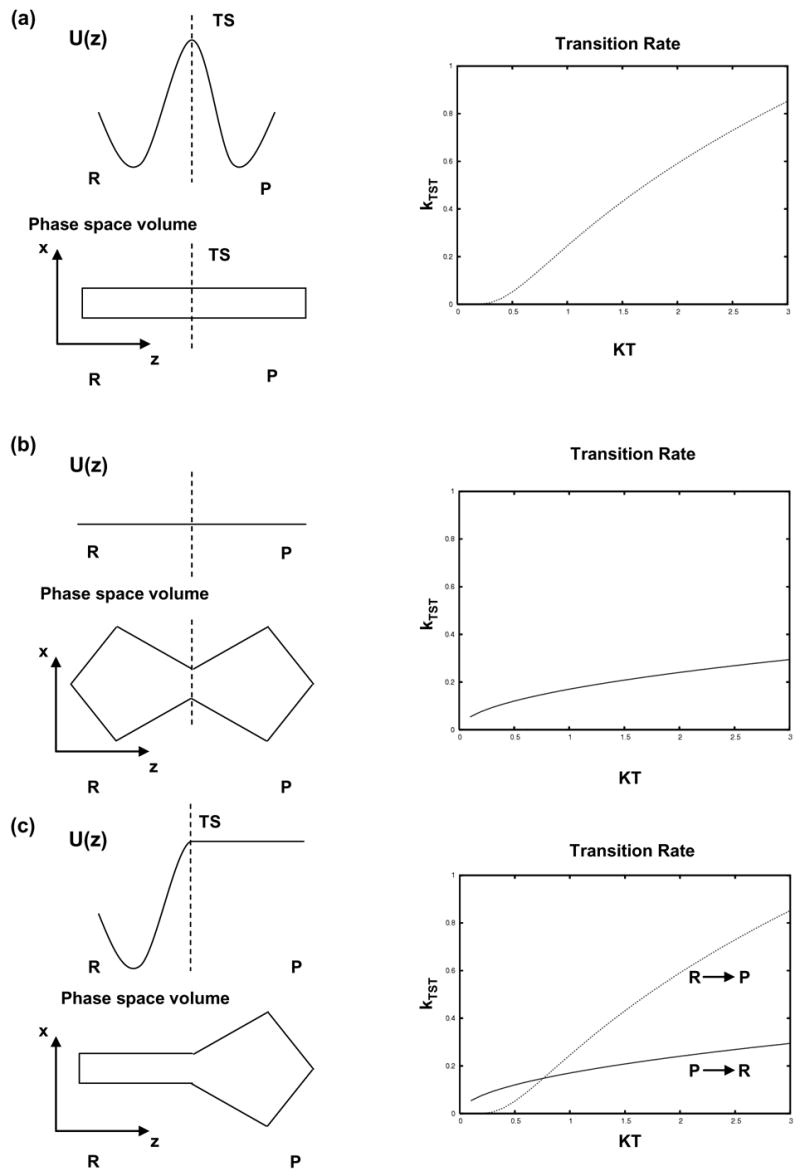
(a) A purely enthalpic barrier. (b) An entropic barrier. (c) A mixed enthalpic/entropic barrier.
| [1] |
The free energy profile is simply
| [2] |
The transition state theory (TST) (Hanggi et al. 1990) estimate of the crossing rate is
| [3] |
| [4] |
The TST estimate increases pseudo-exponentially as the temperature is raised (Figure 1a).
Now consider the system shown in Figure 1b. In this case the system is confined to an irregular shaped box defined by
| [5] |
There is no potential energy gradient within the available phase space, but there is still a free energy gradient because the “breadth” of phase space varies with the reaction coordinate. The free energy profile for this system is
| [6] |
where Δx(z) is the width of the available phase space as a function of the reaction coordinate. Employing [6] in [3] for the phase space defined by [5] yields
| [7] |
In this case the transition rate only increases as T1/2. Figure 1c shows a mixed barrier that is entropic on one side, but enthalpic on the other. The temperature has a greater impact on the R→P transitions than the P→R transitions.
The protein folding barrier may bear some resemblance to this mixed barrier. Entropy is lost along the denatured state → transition state (D → TS) portion of the folding pathway, followed by a favorable change in enthalpy along the transition state → native state (TS → N) portion of the pathway (Jackson and Fersht 1991; Li and Daggett 1994; Fersht 1999). The unfolding rate increases much more dramatically with temperature than the folding rate (Fersht 1999). In molecular simulations at elevated temperatures protein unfolding can occur within a few ns (Daggett 2002; Day et al. 2002). Relative to the simulation time, the folding reaction is very slow at any reasonable temperature. Another example is the engrailed homeodomain, which is a so-called ultrafast folding protein. This protein unfolds on the ns timescale by both simulation and experiment at 348 K, yet it folds in approximately 15 μs (Mayor et al. 2003).
The literature contains REMD studies of peptides (Sugita and Okamoto 1999; Garcia and Sanbonmatsu 2001; Zhou et al. 2001; Nymeyer and Garcia 2003; Gnanakaran et al. 2004; Jas and Kuczera 2004; Andrec et al. 2005; Paschek et al. 2005; Sugita and Okamoto 2005), protein A (Garcia and Onuchic 2003), the BBA5 mini-protein (Rhee and Pande 2003), and the Trp-cage mini-protein (Pitera and Swope 2003; Zhou 2003). An REMD simulation with N replicas is at least as computationally expensive as performing a conventional simulation N times, where normally N ranges from 25–100. Due to the cost of performing so many all-atom, explicit solvent replica simulations, the REMD simulation time in this study for the Trp-cage mini-protein is 10 ns per replica, which translates into 1.42 μs of MD (two REMD simulations with 71 replicas each and 10 ns of sampling for each). While this represents the most extensive REMD study of a solvated protein to date, one wonders whether it is reasonable to expect an explicit solvent REMD simulation of this mini-protein to equilibrate on this timescale given that it folds in approximately 4 μs (Qiu et al. 2002). When implicit solvent models are used and there are no water molecules to rearrange or move, the protein dynamics timescales are altered and equilibration may occur on a non-physical timescale, such as 10 ns, but this is at the expense of realism since protein conformation is very sensitive to the solvent environment.
A simple test for equilibration is whether multiple simulations, starting from different initial conditions, will converge to the same steady state conditions. This test was used to confirm equilibration of REMD simulations of an alanine trimer (Sugita et al. 2000). It has also been used to test for convergence in REMD simulations of a 21-residue helical peptide (Zhang et al. 2005). However, in that case, an implicit solvent model was used and convergence occurred on a non-physical timescale of about a nanosecond. In another study using a modified REMD method the authors dubbed Multiplexed REMD (MREMD), convergence was not observed for the BBA5 mini-protein despite having 200 microseconds of aggregate simulation time in blocks of tens of nanoseconds of continuous implicit solvent simulations (Rhee and Pande 2003). Here we report, two separate REMD simulations using the same protein, explicit water model, and simulation protocols, but very different starting conformations. The protein of interest is Trp-cage, a designed 20-residue mini-protein in which an N-terminal helix packs against a C-terminal polyproline chain, burying a Trp residue on the helix in the protein interior (Neidigh et al. 2002). Trp-cage is an attractive model for computational studies, not only because of its size, but because its structure was predicted to within 1.0 Å Cα root-mean-squared-deviation (RMSD) by MD simulation before the nuclear magnetic resonance (NMR) nuclear Overhauser effect crosspeaks (NOEs) were assigned (Simmerling et al., 2002). The Trp-cage protein has already been studied twice before by REMD (Pitera and Swope 2003; Zhou 2003). The mutant we consider here, tcb, is 95% folded in water at 280 K, although the melting temperature is only 315 K (Neidigh et al. 2002; Qiu et al. 2002).
The first REMD simulation reported here was initiated from the native state, at all replica temperatures and will be referred to as ‘native REMD’. Over the first few ns it gave results that are qualitatively similar to the earlier published REMD simulations, including an unrealistic estimate of the melting temperature, approximately 360 to 460 K. However, as the simulation progressed to 10 ns, the protein slowly unfolded at all replica temperatures. In the REMD simulation starting from the nonnative state, referred to as ‘nonnative REMD’, no significant folding was observed over 10 ns. These simulations did not converge on the same steady state conditions and therefore did not equilibrate over their combined 1.42 μs simulation time. Due to the replica exchange process, these simulations do not yield continuous trajectories that can be used to characterize Trp-cages folding/unfolding pathway.
We also report 16 conventional MD simulations at temperatures ranging from 278 K to 498 K for an aggregate simulation time of 1.032 μs. In the 278 K simulations the protein remained close to the native state. These simulations were from 30–100 ns long. They provided enough sampling to see the protein unfolding by a variety of metrics at higher temperatures, e.g., 348, 373, 448 and 498 K. However, the simulations were not long enough to witness spontaneous refolding at these temperatures given that the unfolding rate dominates. The conventional simulations provide a more reliable estimate of the melting temperature (310 K to 323 K) than the REMD simulations for less than half of the computational cost. In addition, they also provide a continuous trajectory that can be used to describe conformational transitions at atomic resolution.
2. Methods
We performed two separate REMD simulations with 71 replicas, each at energy levels roughly corresponding to temperatures ranging from 280 K to 560 K. Each simulation was performed for 10 ns, such that the total simulation time of all replicas for both REMD simulations was 1.42 μs. For comparison with the REMD simulations, we performed conventional simulations, two each, across a range of temperatures: 278, 298, 310, 315, 323, 348, 373, and 498 K. The simulations at each temperature were the following lengths: 50, 50, 40, 40, 30, 35, 40, and 90 ns, respectively. The total simulation time was 750 ns. For the native REMD simulation, as well as the conventional MD simulations, the starting structure was the 1st of the 20-member NMR structural ensemble (Neidigh et al. 2002) (pdb code: 1L2Y). The second REMD simulation started from a nonnative structure, which was the 50 ns structure in a simulation of the aforementioned NMR structure at 498 K. The Cα RMSD between the native and nonnative REMD starting structures is 7.4 Å.
All simulations were performed with the Levitt et. al. (1995) protein potential function and the flexible F3C water model (Levitt et al. 1997), using the in lucem Molecule Mechanics (ilmm) program (Beck et al., 2006). The generic protocols have been described previously (Beck and Daggett 2004). To generate the starting coordinates and velocities of the lowest temperature replica (280 K), the starting structure (i.e. the NMR structure for the native REMD simulation or the nonnative REMD simulation) was steepest descents (SD) minimized for 1000 steps, and then solvated in a box of water at 0.99983 g/ml, approximately the experimental density of water at 280 K (Kell 1967; Haar et al. 1984). The water box size was bigger in the second REMD simulation because its starting structure was expanded relative to the native state. The native and nonnative REMD simulations had 1539 and 1932 waters, respectively. The water network in the system was SD minimized for 1000 steps, and then the water was simulated for 1 ps, during which the water temperature was raised from 0 to 35 K by our standard heating protocol (Beck and Daggett 2004). Following that, another 1000 steps of SD minimization of the water network was performed. The protein was subjected to 500 steps of SD minimization. Finally, the entire system was simulated for 35 ps to bring it to approximately 280 K. The resulting coordinates and velocities were used to initiate the first, lowest energy replica. The conventional MD simulations were initiated in a similar fashion with standard protocols (Beck and Daggett 2004). A 10 Å nonbonded cutoff updated every time step was used and 1–4 nonbonded interactions were included and scaled by 0.4 (cscale).
The starting coordinates and velocities of the other replicas in the REMD simulations were generated by an iterative scheme: to initiate the kth replica, the box size was increased such that the water density matched the experimental density for the desired temperature, where available (Kell 1967; Haar et al. 1984). Linear interpolation between experimental densities for target temperatures not reported (Kell 1967; Haar et al. 1984) was used in other cases. The target temperature, (280 + 4*k) K, was determined on the assumption that the net kinetic energy gain (after equilibration) is equal to half the total energy input in the system. The velocities of the k-1 replica were scaled such that the total kinetic energy increased by 4 K. The equipartition theorem states that this assumption would be correct if the potential function were harmonic (Plishke et al. 1994). The kth replica was then simulated for 5 ps before the k+1 replica was generated.
REMD was originally developed for an NPT ensemble, for which the sampling of configurations is Boltzman distributed. The exchange process is designed to maintain this distribution at each energy/temperature level. Neighboring replicas are selected at random and exchanged with an exchange probability (Sugita and Okamoto 1999):
| (8) |
where β=1/kBT, β’=1/kBT’, T, T’ are the temperatures, U is the potential function, and x, x’ are the system coordinates in the respective replicas. Our simulations were performed using the NVE ensemble (Beck and Daggett 2004), for which the sampled configurations lie on a constant energy surface. We developed a different exchange process that is appropriate for this ensemble. First, a pair of neighboring replicas was selected at random. The box size of each replica was scaled to match the new box size (i.e. the box size of the neighbor pre-exchange) such that the experimental densities of water at the replicas’ temperature were maintained. The coordinates were also scaled by the same factor as the box size, and the potential energy was calculated. The systems’ velocities were then scaled such that the total system energy matched the new energy level.
The rate of replica exchange is an adjustable parameter that affects equilibration of the replica ensemble. Ideally the rate is fast enough to allow replicas to traverse many times between high and low temperature regimes, but slow enough that adequate relaxation occurs after each exchange. For both REMD simulations, we performed 27 exchanges at each ps. That is, 27 sets of neighbors were selected for exchange once a ps such that any individual replica had approximately a 76% change of exchange. On average, each replica experienced 7500 exchanges over the 10 ns of simulation time.
These exchange rates were determined by two previous Trp-cage REMD simulations conducted in our lab of native and nonnative structures for 7 and 4 ns, respectively (unpublished). During these earlier REMD simulations, the exchange rate was varied from 5/ps to 35/ps. The lower values yielded exchange rates that were too slow to achieve complete traversal of the temperature space while the highest value permitted minimal relaxation after each exchange. Our choice of 27 exchanges per ps allowed replicas, on average, slightly more than a full ps to relax after a change in mean temperature of 4 K. It was also fast enough to ensure that every replica explored the highest and lowest temperature regimes in its 10 ns sampling time. The simulation protocols employed here are compared with those of Zhou (Zhou 2003) and Pitera and Swope (Pitera and Swope 2003) in Table 1.
Table 1.
Summary of simulation protocols for several REMD simulations of Trp-cage
| Simulation | Starting Structure | Simulation Time per Replica | # of Replicas | Temperature Range | # of Exchanges (approx) | Solvent | Force Field |
|---|---|---|---|---|---|---|---|
| Native REMD | Native | 10 ns | 71 | 280K–560K | 270,000 | Explicit | Levitt et al. |
| Nonnative REMD | Nonnative | 10 ns | 71 | 280K–560K | 270,000 | Explicit | Levitt et al. |
| Zhou (2003) | Native | 5 ns | 50 | 282K–598K | 4000 | Explicit | OPLSAA |
| Pitera and Swope (2003) | Extended | 4 ns | 25 | 250K–630K | unknown | Implicit | Amber 94 |
3. Results and Discussion
One advantage of constant energy simulations is that energy conservation itself can be used to evaluate the simulation protocols (Beck and Daggett 2004). Figure 2 shows the total energy of each replica and its corresponding temperature range. The total energy of the replicas ranged from −11,753 to 152 kcal/mol in the native REMD simulation, and from −14,741 to 32 kcal/mol in the nonnative run. The difference in total energy between the two REMD simulations is due primarily to the differences in the number of water molecules. In both, the standard deviation in energy for all replicas is less than 0.1%, and there is no evidence of energy drift over the course of the simulations. Thus, energy is well conserved by the exchange process. The instantaneous temperature may be expected to fluctuate. The standard deviation in temperature is less than 4%. No drift was observed in the average temperature at any energy level. Of particular importance, the average temperatures of the low-to-moderate temperature replicas (280–400 K) matched the “target” temperatures (which were used to set the simulation box size) to within 8 K, often to within 5 K. This means that the simulation densities were close to the relevant experimental values. The average temperatures of the high temperature replicas (>500 K) were as much as 12 K higher than the “target” temperatures. However, these replicas were only included to improve, sampling and were not meant to correspond to reality.
Figure 2. Total system energy as a function of replica mean temperature for REMD simulations.
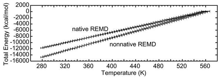
Temperature error bars are shown as standard deviation for each replica. Neighboring replicas overlap by less than 5 K at very high temperatures and less than 2 K at low temperatures. The difference in system energy for the two REMD runs is a result of the native and nonnative starting structures having different box sizes and therefore different numbers of waters.
REMD generates ensembles of configurations (presumably equilibrium ensembles) at different temperatures. These simulations are often used to produce melting curves that depict the fraction of folded or native structures as a function of temperature. Folding rates cannot be measured since the dynamical information is distorted by the exchange process. Unfortunately, many of the experimental measurements of protein stability, such as Trp fluorescence and calorimetric data, cannot be reliably estimated from structural ensembles. Correlations between experiment and structure, for instance between CD and secondary structure or between Trp fluorescence yield and the solvent accessible surface area (SASA) of the Trp residues, are not easy to quantify and often quite specific to the system under study. Thus, the folded content of an ensemble of simulation structures is usually based on a structural criterion that is not directly measurable by experiment. This criterion is always arbitrary to some degree and generally depends on adjustable parameters.
Pitera and Swope (2003) used a cutoff of 2 Å Cα RMSD from the NMR structures to define the folded state, and they obtained a melting temperature of 400 K (Table 2). CD and Trp fluorescence experiments determined the melting temperature to be 315 K (Qiu et al. 2002). At low temperatures, the majority of the REMD simulation structures generated here had a Cα RMSD from the native state > 2 Å (Figure 3a). In contrast, the average Cα RMSD of our conventional 278 K simulations was ≈ 1.2 Å. Using Pitera and Swope’s cutoff, the Tm from the conventional simulation is 315 K (Figure 3a).
Table 2.
Estimates of the melting temperature of the Trp-cage protein. We estimated the melting temperatures by visual inspection of figures such as those in Figure 3, which shows the average values of different folding metrics.
| Source | Metric | Temperature |
|---|---|---|
| Experiment (Neidigh et al. 2002; Qiu et al. 2002) | Tryptophan fluoresence
CD NMR chemical shifts |
315 K |
| Conventional MD | Cα RMSD
Native Contacts Trp 6 SASA Long-range NOEs |
310–315 K
310–323 K 325–348 K 315–323 K |
| Native REMD | Cα RMSD
Native Contacts Trp 6 SASA Long-range NOEs |
N/A
N/A N/A N/A |
| Nonnative REMD | Cα RMSD
Native Contacts Trp 6 SASA |
N/A
N/A N/A |
| REMD (Pitera and Swope 2003) | Cα RMSD | 380 K |
| REMD (Zhou 2003) | Native Contacts | 440 K |
Figure 3. Average values of various folding metrics as a function of temperature/simulation time for the native REMD simulation and the conventional simulations.
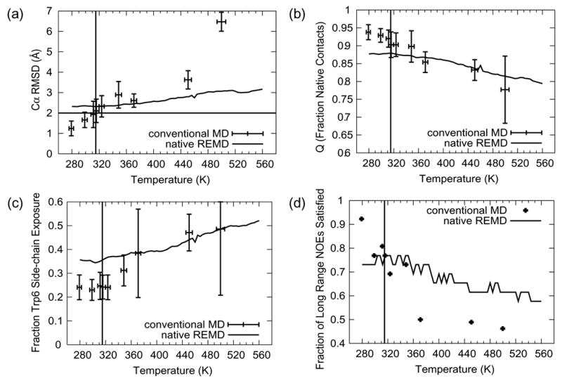
For each conventional simulation the averaging interval was the final 10 ns of the simulation time. The vertical line in each panel is located at 315 K, the melting temperature from experiment (Qiu et al. 2002). (a) Cα RMSD from the SD minimized first of 20 member NMR models (Neidigh et al. 2002) (PDB code 1L2Y) with a horizontal line at 2.0 Å, the metric employed by Pitera and Swope (Pitera and Swope 2003) to denote the folded to unfolded transition. (b) Q, the fraction of native contacts. Two heavy atoms are considered to be in contact if they are within for 4.6 Å of each other (or within 5.4 Å if one or both of the atoms is a carbon atom). c) Side-chain SASA of the Trp 6 residue, calculated using the algorithm of Lee and Richards (Lee and Richards 1971) normalized by the mean side-chain SASA of the central Trp from a 100 ns simulation of GGWGG at 298 K. The GGWGG side-chain SASA reflects a fully exposed Trp.
The criterion to designate a structure as folded or unfolded used by Zhou (2003) was the average fraction of native contacts at each temperature. Their contact definition was more forgiving than ours, i.e. 6.5 Å pair separation between atom centers but they required 100% of the native contacts to be present in order to quantify a conformation as folded. Rather, we use a stricter cutoff definition, but expect contacts to fluctuate as they do under normal solution state dynamics. A loss of about 10% of the native residue based contacts is sufficient to alter the structure and yield conformations that satisfy about 75% of the long range NOEs (Figure 3, panels b and d). Averaged over the 10 ns of both the REMD simulations, the protein was never folded by this metric (Figure 3b) and therefore prevented us from estimating the Tm from the REMD simulations by Q. The Tm for the conventional MD simulations by this metric was 310–323 K.
The fraction of Trp 6 exposure from our conventional and REMD simulations is presented in Figure 3c. The side-chain SASA (Lee and Richards 1971) from the simulations is normalized against the value of Trp’s side-chain SASA derived from a 100 ns simulation of GGWGG performed at 298 K with the same methods as those employed in this study (data not presented). While there isn’t a precise cutoff in SASA or fractional exposure that is rigorously linked to fluorescence, it is evident that the conventional MD simulations undergo a change in Trp exposure in the region of the experimental Tm. Again it is difficult to determine the Tm in the REMD simulation, as it is either less than 278 K, since the protein native state is not modeled adequately under folding conditions with this method, or the Tm is around 440 K.
Comparison with experimental NOEs is a useful tool for validation of a simulation and for assessing the extent of conformational sampling. For the purposes of this study, an NOE was satisfied if the r−6 weighted sum of proton distances was less than the upper bound distance in the published NOE set from the PDB. There are 169 NOEs available for the Trp-cage protein at 280 K, 26 of which are long range (i → i + 5 or greater) (Neidigh et al. 2002). Figure 3d shows the percentage of long range NOE violations as a function of temperature for the conventional MD runs and the native REMD simulation. At low and intermediate temperatures the number of violations of all NOEs was qualitatively similar to that observed by Zhou (Zhou 2003) and Pitera and Swope (Pitera and Swope 2003). Contrast this with the conventional simulations, below the Tm, that exhibited excellent agreement with the NOEs: satisfying 98 % of the 169 NOEs at 278 K. Not surprisingly, the conventional simulations at higher temperatures, i.e. those above the protein’s melting temperature, did not agree with the NOEs as well as the REMD simulations at the same temperatures.
Overall, the study of various folding metrics (Table 2, Figure 3), including the solvent-exposed surface area of Trp 6, suggested that neither REMD simulation sufficiently sampled the folded state at any temperature. The snapshots of the Trp-cage protein in Figure 4 from NMR, conventional MD and REMD illustrate this point. The conventional MD simulations in Figure 4b exhibit levels of structural heterogeneity consistent with the simulation temperature. In Figure 4c, the replicas were slowly unfolding through the course of the simulation in the case of the native REMD simulations. While in Figure 4d, the nonnative simulation continued to sample the unfolded conformational states local to the starting structure.
Figure 4. Snapshots of Trp-cage mini-protein from NMR, conventional MD and REMD simulations at temperatures corresponding to folded, Tm, and unfolded conditions.
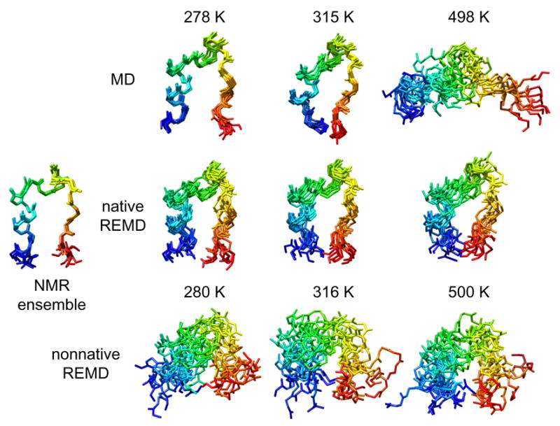
(a) The first 10 models from the NMR structures (Neidigh et al. 2002) (PDB code 1L2Y). (b) The final 10 ns at 1 ns granularity from 278, 315, and 498 K simulations. (c) and (d) Ten structures at 1 ns granularity from 280, 316 and 500 K replicas of REMD simulations starting from (c) a native structure and (d) a nonnative structure. The protein main-chain is shown colored from blue (N-terminus) to red (C-terminus). Image rendered with UCSF Chimera (Pettersen et al. 2004).
In Figure 5, histograms of the Cα RMSD from (a) the conventional MD simulations and (b) the native REMD run are presented for different temperatures. It is interesting to note that in panel (a) there are clean delineations between the native and nonnative conformations at 278 and 498 K. The 315 K distribution is bi-modal with one peak in the native range and another just over the 2 Å cutoff identified by Pitera and Swope (Pitera and Swope 2003). This behavior is indicative of partial unfolding and the protein in these simulations is sampling both folded and unfolded states, as would be expected at simulations around the Tm. This type of delineation is not seen in the REMD simulations in panel (b) where the distributions are very similar for the three temperatures presented. Thus, the conventional simulations yield folded structures at low T and more disrupted structures with increasing temperature. The REMD simulations give slightly disrupted structures at all temperatures, meaning that they are too unfolded under native conditions and too folded at higher temperatures.
Figure 5. Histograms of Cα RMSD as a function of temperature for conventional MD and REMD simulations.
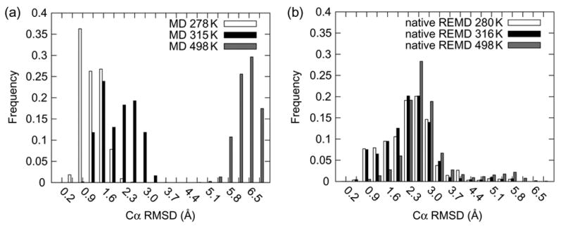
(a) Histograms of Cα RMSD for the final 10 ns of the conventional MD simulations performed at 278, 315 and 498 K. Notice the clear delineation of native and nonnative conformers at about 2 Å, the value used by Pitera and Swope (Pitera and Swope 2003) to denote folded and unfolded states. The 278 and 498 K simulations, below and above Trp- cage’s Tm, respectively, yield mean Cα RMSD’s corresponding to native and nonnative states by this definition. The 315 K simulation, at the experimentally determined Tm (Neidigh et al. 2002; Qiu et al. 2002) exhibited a bi-modal distribution just inside and outside the native cutoff. (b) Histograms of Cα RMSD from the native REMD simulation from the 280, 316 and 500 K replicas. These distributions overlap significantly and do not reflect temperature dependent conformational sampling.
The Cα RMSD increased over the course of the native simulation (Figure 6a). In the nonnative REMD simulation the replicas started from extended structures, and exhibited no obvious signs of folding over 10 ns (Figures 4 and 6b). The two simulations gave completely different results with respect to all of the metrics presented. As an example, Figure 6 depicts the native and nonnative REMD Cα RMSD. Clearly equilibration as measured by convergence of both simulations on the same steady state condition was not achieved over the short simulation time of 10 ns per replica (from a total of 0.71 μs of sampling per REMD simulation).
Figure 6. Trp-cage Cα RMSD as a function of REMD replica temperature and sampling interval.
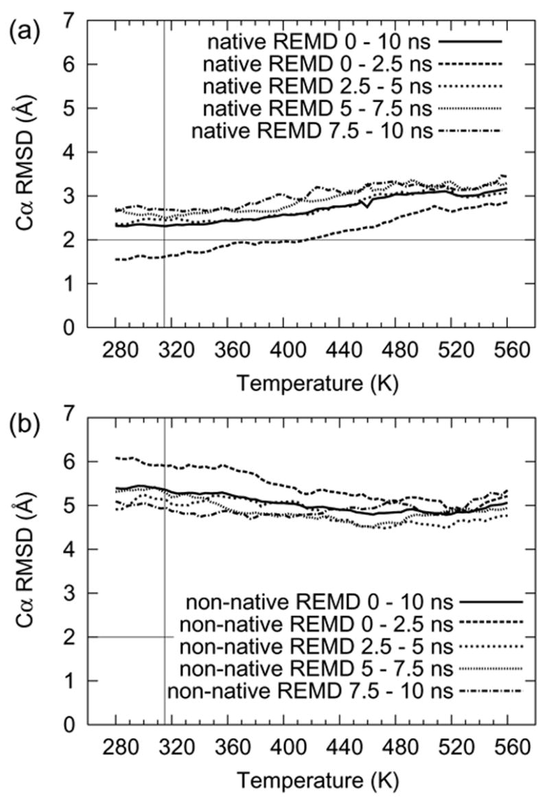
(a) Data from the native REMD simulation. The initial 2.5 ns time period of the simulation demonstrated folded and unfolded conformers by the Pitera and Swope metric of 2 Å Cα RMSD. From this time domain the Tm can be estimated at about 360 K. However, as the REMD simulation progressed, the protein began to unfold at all replicas. As the time approaches the end of the simulation, the RMSD continues to rise, though more slowly. (b) Data from the nonnative REMD simulation. The RMSD from the start and end time regimes show little difference and no significant change towards the native state conformations. The native and nonnative REMD simulations do not converge on the same steady state conditions over their combined 1.42 μs of sampling time.
The REMD simulation of Zhou (2003) was 5 ns per replica, although the author acknowledged that this may not have been adequate to achieve equilibration. As discussed above, the equilibration rate depends to some degree on the exchange rate. The reported exchange rate suggests that there were only about 4000 exchanges over the course of Zhou’s 5 ns simulation. Thus, each replica made 160 pseudo-random “steps” in temperature space. The RMS distance traveled by each replica was about 13, which is insufficient to cover a space of 50 units (i.e. the number of temperature levels in the simulation). The exchange rate used here was about 30 times faster.
Implicit solvent models can accelerate protein dynamics by orders of magnitude, and a large degree of folding clearly occurred in the REMD simulation of Pitera and Swope (Pitera and Swope 2003), which was only 4 ns long. Furthermore, Swope and Pitera report that calculations over the final ns of the simulation were similar to calculations over the final 2 ns, suggesting that equilibrium was achieved. Although the native state structure was reproduced by this simulation, agreement with the experimentally determined melting curve was poor. That was true of Zhou’s simulations, as well, and he postulated that it was due to problems with the force field. Accordingly, Simmerling and co-workers (2002) originally solved the structure at a temperature of 348 K, which is 33 K higher than the melting temperature, suggesting that some reparameterization of the force field may be in order. Overall the findings of the earlier Trp-cage studies suggest that the balance determining the thermodynamic behavior of the protein may not be accurate, which could be due to a variety of factors. Given that we obtain good agreement with the experimental Tm with conventional MD but not with REMD simulations and that the same force field is employed for both sets of simulations, we believe that it is a limitation of the REMD method.
The conventional simulations ran for much longer (in some cases as much as 80 ns longer) than the individual replica simulations. Nevertheless, the simulation times were still much shorter than the folding and unfolding times (4.1 and 12.7 μs, respectively at 296 K (Qiu et al. 2002)), and ideally they should be comparable to, or many times greater than, the folding/unfolding times to achieve equilibration between the native and unfolded states. The protein was folded in two simulations at 278 K and unfolded in simulations at 348, 373, 348, and 498 K, which are all well above the experimental melting temperature (Figures 3 and 4). In the simulations at intermediate temperatures (298–323 K), where experimentally both native and unfolded states are well populated, the values of the folding metrics were scattered, although there was some correlation with temperature (Figures 4 and 5). The conventional simulations suggest that the melting temperature is somewhere between 310–323 K. Estimates that are significantly less than the 360–400 K range of previous studies (Pitera and Swope 2003; Zhou 2003). Thus, the conventional MD simulations provide better estimates of the melting temperature than either of the REMD simulations for much less computational effort. Furthermore, the conventional simulations provide continuous pathways for conformational transitions, such that one can address kinetic pathways of folding and unfolding, which cannot be done with the discontinuous REMD simulations even if they were to reproduce thermodynamic sampling.
5. Conclusions
The replica-exchange method was developed to overcome dynamical bottlenecks that are significant at low temperatures but not at high temperatures, such as those caused by potential energy barriers. However, the barrier(s) between the protein native and denatured states are partially entropic. Protein folding rates derived from experiment do not increase as rapidly as unfolding rates with increasing temperature (Fersht 1999), and simulations with explicit solvent have never led to protein folding on a nanosecond time scale. Protein folding is a slow process (relative to simulation time) at both low and high temperatures. Simple secondary structure motifs such as hairpin turns may require several μs to form. Therefore, it is probably unreasonable to expect that exchanges between simulations at different temperatures would lead to rapid equilibration between the native and denatured states in an explicit solvent simulation. Implicit solvent may be used to accelerate the system dynamics, but can also distort the equilibrium properties (such as the thermal stability). Future work in this area could extend the explicit solvent REMD simulation time, but several orders of magnitude may be required. Given the tendency toward disrupted structures at all temperatures with increasing simulation time, the thermodynamic behavior may not improve. Also, it may take several orders of magnitude increase in simulation time with REMD, but conventional MD has already been shown to be more computational efficient and it can already produce experimentally reasonable results without the need for such extensive sampling.
So, even in cases where REMD seems to "work", it may not be better than the judicious selection of temperatures for an array of conventional simulations. The computational overhead of simulating at a tightly spaced array of temperatures may not be worthwhile when a select, properly spaced set of temperatures can be treated in a conventional manner. Furthermore, conventional simulations provide insight into system dynamics, such as protein folding/unfolding, due to the continuity of the trajectory in phase space. Overall we find conventional MD to be superior to REMD with respect to efficient use of computational resources, ability to reproduce experiment, and the insight provided into time-dependent conformational behavior.
Acknowledgments
We thank Drs. Darwin O.V. Alonso, Niels H. Andersen, and Carlos Simmering for helpful discussions.
Footnotes
Publisher's Disclaimer: This is a PDF file of an unedited manuscript that has been accepted for publication. As a service to our customers we are providing this early version of the manuscript. The manuscript will undergo copyediting, typesetting, and review of the resulting proof before it is published in its final citable form. Please note that during the production process errors may be discovered which could affect the content, and all legal disclaimers that apply to the journal pertain.
References
- Andrec M, Felts AK, Gallicchio E, Levy RM. Protein folding pathways from replica exchange simulations and a kinetic network model. Proc Natl Acad Sci U S A. 2005;102:6801–6806. doi: 10.1073/pnas.0408970102. [DOI] [PMC free article] [PubMed] [Google Scholar]
- Beck DAC, Daggett V. Methods for Molecular Dynamics Simulations of Protein Folding/Unfolding in Solution. Methods. 2004;34:112–120. doi: 10.1016/j.ymeth.2004.03.008. [DOI] [PubMed] [Google Scholar]
- Daggett V. Molecular dynamics simulations of the protein unfolding/folding reaction. Acc Chem Res. 2002;35:422–429. doi: 10.1021/ar0100834. [DOI] [PubMed] [Google Scholar]
- Day R, Bennion BJ, Ham S, Daggett V. Increasing temperature accelerates protein unfolding without changing the pathway of unfolding. J Mol Biol. 2002;322:189–203. doi: 10.1016/s0022-2836(02)00672-1. [DOI] [PubMed] [Google Scholar]
- Fersht A. Structure and mechanism in protein science: a guide to enzyme catalysis and protein folding. New York: W.H. Freeman; 1999. [Google Scholar]
- Garcia AE, Onuchic JN. Folding a protein in a computer: An atomic description of the folding/unfolding of protein A. Proc Natl Acad Sci U S A. 2003;100:13898–13903. doi: 10.1073/pnas.2335541100. [DOI] [PMC free article] [PubMed] [Google Scholar]
- Garcia AE, Sanbonmatsu KY. Exploring the energy landscape of a beta hairpin in explicit solvent. Proteins-Structure Function and Genetics. 2001;42:345–354. doi: 10.1002/1097-0134(20010215)42:3<345::aid-prot50>3.0.co;2-h. [DOI] [PubMed] [Google Scholar]
- Gnanakaran S, Hochstrasser RM, Garcia AE. Nature of structural inhomogeneities on folding a helix and their influence on spectral measurements. Proc Natl Acad Sci U S A. 2004;101:9229–9234. doi: 10.1073/pnas.0402933101. [DOI] [PMC free article] [PubMed] [Google Scholar]
- Haar L, Gallagher JS, Kell GS. NBS/NRC Steam Tables. New York: Hemisphere; 1984. [Google Scholar]
- Hanggi P, Talkner P, Borkovec M. Reaction-Rate Theory - 50 Years after Kramers. Rev Mod Phys. 1990;62:251–341. [Google Scholar]
- Jackson SE, Fersht AR. Folding of Chymotrypsin Inhibitor-2.1. Evidence for a 2-State Transition. Biochemistry. 1991;30:10428–10435. doi: 10.1021/bi00107a010. [DOI] [PubMed] [Google Scholar]
- Jas GS, Kuczera K. Equilibrium structure and folding of a helix-forming peptide: Circular dichroism measurements and replica-exchange molecular dynamics simulations. Biophys J. 2004;87:3786–3798. doi: 10.1529/biophysj.104.045419. [DOI] [PMC free article] [PubMed] [Google Scholar]
- Kell GS. J Chem Eng Data. 1967;12:66. [Google Scholar]
- Lee B, Richards FM. Interpretation of Protein Structures - Estimation of Static Accessibility. J Mol Biol. 1971;55:379. doi: 10.1016/0022-2836(71)90324-x. [DOI] [PubMed] [Google Scholar]
- Levitt M, Hirshberg M, Sharon R, Laidig KE, Daggett V. Calibration and testing of a water model for simulation of the molecular dynamics of proteins and nucleic acids in solution. J Phys Chem B. 1997;101:5051–5061. [Google Scholar]
- Li A, Daggett V. Characterization of the transition state of protein unfolding by use of molecular dynamics: chymotrypsin inhibitor 2. Proc Natl Acad Sci U S A. 1994;91:10430–4. doi: 10.1073/pnas.91.22.10430. [DOI] [PMC free article] [PubMed] [Google Scholar]
- Mayor U, Guydosh NR, Johnson CM, Grossmann JG, Sato S, Jas GS, Freund SM, Alonso DOV, Daggett V, Fersht AR. The complete folding pathway of a protein from nanoseconds to microseconds. Nature. 2003;421:863–7. doi: 10.1038/nature01428. [DOI] [PubMed] [Google Scholar]
- Neidigh JW, Fesinmeyer RM, Andersen NH. Designing a 20-residue protein. Nat Struct Biol. 2002;9:425–430. doi: 10.1038/nsb798. [DOI] [PubMed] [Google Scholar]
- Nymeyer H, Garcia AE. Simulation of the folding equilibrium of alpha-helical peptides: A comparison of the generalized born approximation with explicit solvent. Proc Natl Acad Sci U S A. 2003;100:13934–13939. doi: 10.1073/pnas.2232868100. [DOI] [PMC free article] [PubMed] [Google Scholar]
- Paschek D, Gnanakaran S, Garcia AE. Simulations of the pressure and temperature unfolding of an alpha-helical peptide. Proc Natl Acad Sci U S A. 2005;102:6765–6770. doi: 10.1073/pnas.0408527102. [DOI] [PMC free article] [PubMed] [Google Scholar]
- Pettersen EF, Goddard TD, Huang CC, Couch GS, Greenblatt DM, Meng EC, Ferrin TE. UCSF chimera - A visualization system for exploratory research and analysis. J Comput Chem. 2004;25:1605–1612. doi: 10.1002/jcc.20084. [DOI] [PubMed] [Google Scholar]
- Pitera JW, Swope W. Understanding folding and design: Replica-exchange simulations of "Trp-cage" fly miniproteins. Proc Natl Acad Sci U S A. 2003;100:7587–7592. doi: 10.1073/pnas.1330954100. [DOI] [PMC free article] [PubMed] [Google Scholar]
- Plishke M, Bergersen, Birger . Equilibrium Statistical Physics. Singapore: World Scientific Publishing Co; 1994. [Google Scholar]
- Qiu LL, Pabit SA, Roitberg AE, Hagen SJ. Smaller and faster: The 20-residue Trp-cage protein folds in 4 mu s. J Am Chem Soc. 2002;124:12952–12953. doi: 10.1021/ja0279141. [DOI] [PubMed] [Google Scholar]
- Rhee YM, V, Pande S. Multiplexed-replica exchange molecular dynamics method for protein folding simulation. Biophys J. 2003;84:775–86. doi: 10.1016/S0006-3495(03)74897-8. [DOI] [PMC free article] [PubMed] [Google Scholar]
- Sugita Y, Kitao A, Okamoto Y. Multidimensional replica-exchange method for free-energy calculations. J Chem Phys. 2000;113:6042–6051. [Google Scholar]
- Sugita Y, Okamoto Y. Replica-exchange molecular dynamics method for protein folding. Chem Phys Lett. 1999;314:141–151. [Google Scholar]
- Sugita Y, Okamoto Y. Molecular mechanism for stabilizing a short helical peptide studied by generalized-ensemble simulations with explicit solvent. Biophys J. 2005;88:3180–3190. doi: 10.1529/biophysj.104.049429. [DOI] [PMC free article] [PubMed] [Google Scholar]
- Zhang W, Wu C, Duan Y. Convergence of replica exchange molecular dynamics. J Chem Phys. 2005;123 doi: 10.1063/1.2056540. [DOI] [PubMed] [Google Scholar]
- Zhou RH. Trp-cage: Folding free energy landscape in explicit water. Proc Natl Acad Sci U S A. 2003;100:13280–13285. doi: 10.1073/pnas.2233312100. [DOI] [PMC free article] [PubMed] [Google Scholar]
- Zhou RH, Berne BJ, Germain R. The free energy landscape for beta hairpin folding in explicit water. Proc Natl Acad Sci U S A. 2001;98:14931–14936. doi: 10.1073/pnas.201543998. [DOI] [PMC free article] [PubMed] [Google Scholar]