Monitoring and correcting spatio-temporal variations of the MR scanner’s static magnetic field

Abstract

The homogeneity and stability of the static magnetic field are of paramount importance to the accuracy of MR procedures that are sensitive to phase errors and magnetic field inhomogeneity. It is shown that intense gradient utilization in clinical horizontal-bore superconducting MR scanners of three different vendors results in main magnetic fields that vary on a long time scale both spatially and temporally by amounts of order 0.8–2.5 ppm. The observed spatial changes have linear and quadratic variations that are strongest along the z direction. It is shown that the effect of such variations is of sufficient magnitude to completely obfuscate thermal phase shifts measured by proton-resonance frequency-shift MR thermometry and certainly affect accuracy. In addition, field variations cause signal loss and line-broadening in MR spectroscopy, as exemplified by a fourfold line-broadening of metabolites over the course of a 45 min human brain study. The field variations are consistent with resistive heating of the magnet structures. It is concluded that correction strategies are required to compensate for these spatial and temporal field drifts for phase-sensitive MR protocols. It is demonstrated that serial field mapping and phased difference imaging correction protocols can substantially compensate for the drift effects observed in the MR thermometry and spectroscopy experiments.

Introduction

The stability and homogeneity of the main magnetic field are important factors that directly impact the accuracy of MR experiments that are phase sensitive. Phase-based proton-resonance frequency (PRF) MR thermometry measurements are particularly susceptible to underlying field variations [1]. Field homogeneity and stability affect the signal-to-noise ratio (SNR) and resolution in MR spectroscopy. Two major sources of frequency drifts have been identified [2]. First, oscillatory phase drifts that correlate with air-conditioning cycles in the equipment electronic room. These are greatly reduced by advances in receiver electronics. Second, there is the normal drift in the main magnetic field that falls within the magnet’s specifications. This temporal drift is currently treated as spatially homogenous [3]. For PRF thermometry correction primarily involves subtracting the phase of a reference image from the temperature-dependent phase. These also accounts for spatial phase variations due to susceptibility effects [4]. Although the possible existence of phase variations attributable to the main static magnetic field that are both temporal and spatially dependent has been noted, we have found no accounts of the nature, magnitude, or extent of such variations.

Here we show that magnetic field variations are induced by, and directly correlated with, the hardware stress of the MRI system. In particular, the evidence suggests that eddy currents caused by switching gradients result in heating of resistive parts of the MR scanner. We find that the changes in field vary both spatially and temporally in a working, state-of-the-art horizontal-bore clinical MRI systems made by each of GE (1.5 T), Siemens (1.5 T) and Philips (3 T). The observed spatial variations have both linear and quadratic terms that are especially significant in the z direction. We hypothesize that thermal perturbations alter the passive shimming, which in turn results in spatial and temporal field variations. The consequence of such variations on the accuracy of PRF thermometry is demonstrated. The degradation of field homogeneity is manifested as both frequency shifts and spectral line-broadening in single-voxel spectroscopy of a phantom and of a human brain in vivo. Two field (phase) compensation schemes are presented that can successfully correct for the errors produced by the magnet’s spatial/temporal drifts in MR thermometry and spectroscopy experiments. We conclude that serial online or offline field/phase-variation compensation strategies may be essential to the accuracy, stability, and quality control of such experiments.

Theory

Measuring the magnetic field

In a gradient echo (GR) or a spoiled gradient echo (SPGR) MR experiment the sampling/echo acquisition time is small compared to T2 [5]. If the temperature of the imaged subject is not varying, the subject is stationary, a single transmit/receive (T/R) coil is used for acquisition, and if T₂ effects are ignored, then the effect of static field inhomogeneity (ΔB₀) on the reconstructed image intensity, I, is given by

$$I(\mathbf{r},\text{TE})=\parallel M_{\perp }(\mathbf{r})\parallel \cdot {\text{e}}^{-\text{i}\gamma \mathrm{\Delta }{B}_0(\mathbf{r},t)TE+{\phi }_0}$$ (1)

where |M_⊥| is the magnitude of the transverse magnetic field; r is a spatial position vector; γ is the gyromagnetic ratio; TE is the echo time; ΔB₀ is the difference between the local field and the z-component of the main magnetic field B₀ that satisfies the Larmor equation; and φ₀ is the initial (constant) phase. Note that in these experiments any field inhomogeneity primarily affects the phase of the image, whereas in echo-planar sequences [6] it additionally results in image distortion and deformation.

The fact that the image phase contains information about the spatial field distribution is used to calculate true (B₀) field maps by acquiring images at two different echo times (TE₁, TE₂) [7] and determining the difference between their phases [5,8]:

$$\begin{array}{l}\mathrm{\Delta }\phi (\mathbf{r},t,\mathrm{\Delta }\text{TE})=\gamma \mathrm{\Delta }{B}_0(\mathbf{r},t){\text{TE}}_2-\gamma \mathrm{\Delta }{B}_0(\mathbf{r},t){\text{TE}}_1\\ =\gamma \mathrm{\Delta }{B}_0(\mathbf{r},t)\mathrm{\Delta }\text{TE}\end{array}$$ (2)

Therefore,

$$\mathrm{\Delta }{B}_0(\mathbf{r},t)=\frac{\mathrm{\Delta }\phi (\mathbf{r},t,\mathrm{\Delta }\text{TE})}{\mathrm{\Delta }\text{TE}\times \gamma }$$ (3)

where Δφ is the difference in phase, and ΔTE =T E₂ − T E₁. If we reasonably assume that the main magnetic field, and consequently the inhomogeneity term, stays constant during ΔTE, then we may use this method (method A) to measure static field maps and/or to calculate shim values. By measuring ΔB₀ at different time points (t₁, t₂, etc.) over time frames of minutes or hours, the longer-term temporal field variations are determined:

$$\mathrm{\Delta }{B}_0(\mathbf{r},t_2-t_1)=\mathrm{\Delta }{B}_0(\mathbf{r},t_2)-\mathrm{\Delta }{B}_0(\mathbf{r},t_1)$$ (4)

Alternatively, we can utilize the phase difference in images (PDI) that are acquired with the same TE at different time instances to account for field variations (method B):

$$\mathrm{\Delta }\phi (\mathbf{r},t_2-t_1,\text{TE})=\gamma \mathrm{\Delta }{B}_0(\mathbf{r},t_2-t_1)\text{TE}$$ (5)

$$\mathrm{\Delta }{B}_0(\mathbf{r},t_2-t_1)=\frac{\mathrm{\Delta }\phi (\mathbf{r},t_2-t_1,\text{TE})}{\gamma \times \text{TE}}$$ (6)

MR thermometry

We posit that in a GR MR experiment temperature changes of the equipment may result in variations in the field homogeneity. We therefore monitor the magnet homogeneity using either or both of the above methods. The apparent temperature change due to heating,

$$\begin{array}{l}\mathrm{\Delta }T(\mathbf{r},t_2-t_1)=\frac{\mathrm{\Delta }\phi (\mathbf{r},t_2-t_1,\text{TE})}{-\alpha \times \text{TE}\times \gamma \times B_0}\\ =\frac{\mathrm{\Delta }\phi (\mathbf{r},t_2,\mathrm{\Delta }\text{TE})-\mathrm{\Delta }\phi (\mathbf{r},t_1,\mathrm{\Delta }\text{TE})}{-\alpha \times \mathrm{\Delta }\text{TE}\times \gamma \times B_0}\end{array}$$ (7)

with α = −0.01 ppm/°C [9,10], will be superimposed on any magnetic field variations. To compensate for magnetic field variations over the imaged sample volume, we either actively re-shim the magnetic field using the scanners shim gradients [11] or use offline phase-variation compensation.

2D field variation analysis and correction

The spatial variation of the field in planar image acquisitions quantified via Eqs. (4) and (6) for Methods A and B respectively, is quantified and corrected using a two-dimensional (2D) quadratic model. The same model is used for field changes during MR thermometry experiments [8]. The spatial variation of the field is thereby represented as

$$\mathrm{\Delta }{B}_0(r_1,r_2,t_2-t_1)={\alpha }_0+{\alpha }_1{r}_1+{\alpha }_2{r}_2+{\alpha }_3{r}_1^2+{\alpha }_4{r}_2^2+{\alpha }_5{r}_1{r}_2$$ (8)

where r₁ and r₂ are the 2D Cartesian coordinates of r. The α parameters are determined by a least-squares fit which minimizes the root of the sum of the squares (rms) of the difference between the model and the field map (implemented on a PC using Matlab 7, The MathWorks, Inc., Natick, MA).

During MR thermometry at each time point, changes in the phase of a constant-temperature reference that surrounds the phantom serve as measures of phase changes due to spatial variations in the magnetic field. The 2D quadratic model is thus fitted to the spatial variation in the constant temperature reference, and interpolated to the local heating site in order to subtract its effect from the temperature-induced phase measurements [4,12]. This results in a new temperature estimate that is corrected for the field phase-variation effects, (Δφ)_Baseline, and which is suitable for thermal monitoring experiments:

$$\mathrm{\Delta }{T}_C(\mathbf{r},t_2-t_1)=\frac{\mathrm{\Delta }\phi (\mathbf{r},t_2-t_1)-{(\mathrm{\Delta }\phi (\mathbf{r},t_2-t_1))}_{\text{Baseline}}}{-\alpha \times \text{TE}\times \gamma \times B_0}$$ (9)

Spectroscopy

Shimming to optimize the field homogeneity is an essential setup procedure that precedes a MR spectroscopy exam. Signal averaging is commonly used to achieve suitable SNR in vivo. Magnet instability due to heating effects may cause both frequency drift [3] and phase variations that result in SNR loss, line-broadening and the loss of spectral resolution during long averages, or in spectroscopy experiments that are performed serially without re-shimming. The effect can be expressed as

$$S_{\text{avg}}(\omega )=\frac{1}{N}\sum _{i=1}^N{S}_i(\omega +\mathrm{\Delta }{\omega }_i){\text{e}}^{-\text{i}{\phi }_i}$$ (10)

where S_avg is the averaged spectrum, N is the number of averages, S_i is spectral density of the ith acquisition, Δω_i is the frequency drift, and φ_i is the phase.

To demonstrate the effect of field drift on in vivo spectra, proton point-resolved (PRESS) MR spectroscopy [13] is performed in a phantom and the human brain. A localized shimming tool using IDL (Research Systems, Inc., Boulder, CO) is implemented on a PC to correct for static field inhomogeneities [14]. B₀-maps are acquired using Eq. (3), and field inhomogeneities are accounted for up to the second order spherical harmonics in Cartesian coordinates:

$$\begin{array}{l}\mathrm{\Delta }\hspace{0.17em}{B}_0(\mathbf{r},t)=B_{\text{offset}}+G_{x}x+G_{y}y+G_{z}z+G_{xy}xy+G_{xz}xz\\ +\hspace{0.17em}{G}_{yz}yz+G_{x2-y2}(x^2-y^2)\\ +\hspace{0.17em}{G}_{z2}\left(z^2-\frac{x^2+y^2}{2}\right)\end{array}$$ (11)

Shim parameters optimized for a voxel are obtained using a constrained Levenberg–Marquardt least-squares minimization (MINPACK-1: C.B. Markwardt, NASA/GSFC Code 662, Greenbelt, MD 20770) field fit, and fed to the scanner’s shimming coils. Another B₀-map is acquired with the shim corrections applied, to measure the standard deviation (SD) of the remaining inhomogeneity over the voxel in Hz. The change in shim parameters calculated at two or more time points are used to account for the spatial variation of the field with time.

To compensate for field drift occurring during PRESS acquisitions, constructive averaging was employed, wherein a desired peak is identified in the first acquisition, and the remaining acquisitions are phase-shifted based on the average phase of √_N points in the peak prior to averaging [15].

Methods

The static magnetic field homogeneity was monitored on three scanners from three different vendors: (a) a GE Signa 1.5 T scanner with a Desc Conquest 1.5 T magnet manufactured in 1998, equipped with first-order linear shims; (b) a Philips Achieva XMR 3 T scanner manufactured in 2005, equipped with second order quadratic shims; and (c) a Siemens Magnetom mobile MR 1.5 T manufactured in 2004, equipped with first-order linear shims. A single T/R coil was used to avoid possible phase changes associated with temperature dependence of the dielectric constant of the sample (head coils for the GE and Philips systems, and a body coil for the Siemens, for which a T/R head coil was not available). The temperature at the center of the inner surface of the MR scanner bore, and that in the phantom were both monitored using fiber-optic sensors (FISO Technology, Inc., Quebec, Canada). All phantoms are placed at the isocenter of the magnets and, unless otherwise stated, are filled with vegetable oil (100%) whose lipid resonance frequency varies much less with temperature than water [16] in order that any frequency variations will derive predominantly from field changes.

The stability of the electronics and of the magnetic fields without gradient use was first determined in a cylindrical 6-cm-diameter 6-cm-high oil phantom. MR frequency variations were measured by spectroscopic analysis of repeated non-spatially selective free-induction decay acquisitions for up to a 4 h period at a repetition time TR =2 s. The temperature coefficient of the oil was determined from the frequency variation measured in the same way while heating the phantom.

GE experiments

To show a relation between the temperature of the bore and a gradient-intense MR pulse sequence, the temperature of the bore and phantom were monitored with the fiber-optic system while running a balanced steady-state free precession (SSFP) pulse sequence (matrix, 256 × 256; axial slice thickness, ST = 3.5 mm; TR/TE 5.0/1.8 ms; field-of-view, FOV = 28 cm; flip angle, FA = 3°) for 1 h. To view the temporal/spatial magnetic field drift, PDI (method B) was applied while the scanner was cooling down. PDI employed an SPGR pulse sequence which has much less intense gradient transients, with frequency encoding (F_enc) on the x-axis of the scanner’s gradient system (matrix, 256 × 256; TR/TE, 1000/1.8 ms; bandwidth, BW = 125 kHz; FA = 40°; FOV = 32 cm; slice selection and refocusing gradients set to zero; ST given by the phantom thickness was 5 mm). To monitor variations in the x–z (coronal) plane, a 15 cm × 25 cm oil phantom was used. The same sequence with FOV = 28 cm and F_enc on the y-axis was used to monitor variations in the x–y (axial) plane using a circular 15-cm-diameter oil phantom.

Philips experiments

Similar oil phantoms were used for measurements on the Philips 3 T system. Temperature probes were placed in the oil phantom, the bore of the magnet, and on a copper nut connecting the gradient cooling system’s water-return to the chiller. To view the temporal magnetic field drift and spatial variation both PDI (Method B) and true B₀-maps [Eq. (3) and (4); Method A] were performed. The scanner was first heated by applying the same balanced SSFP sequence that was used for the GE scanner for 30–60 min to perturb the system, while the main magnetic field was monitored as the scanner cooled.

Field variations were also measured in the x–z (coronal) plane using PDI applying an SPGR sequence (matrix, 256×256; TR/TE, 300/2.2 ms; FA, 40°; active shim coils; FOV, 28 cm; F_enc along the x-axis; slice selection and refocusing gradient set to zero; ST given by the phantom thickness, 8 mm). The experiment was repeated with the coronal plane rotated 45° about the y-axis and the slice selection gradient turned on, and again with the shim gradients turned off and using B₀-map difference imaging. B₀-maps were also acquired in the x–y (axial) plane (matrix, 256×256; TR/TE₁/TE₂, 150/4/6 ms; FA, 40°; active shim coils; FOV, 25 cm; F_enc, y-axis with axial plane rotated 45°).

Siemens experiment

To confirm that effects occur on yet a third vendor’s system, the oil phantoms were replaced by a 25-cm-diameter spherical saline phantom to properly load the Siemens 1.5 T scanner’s body T/R coil. The scanner was thermally perturbed for 30 min using the same balanced SSFP sequence that was used with the other scanners. The field variation was monitored using PDI with a GR sequence (matrix, 256×256; TR/TE, 80/3.2 ms; FA, 60°; FOV 35 cm; F_enc, x-axis; ST 1 cm).

Temperature monitoring experiments

Two additional thermal monitoring experiments were conducted on the 3 T Philips scanner to directly show the effect of field variations on the accuracy of temperature measurement by PRF MR thermometry. A 15-cm-diameter cylindrical water gel phantom was placed in the center of a birdcage T/R head coil. A dipole heating antenna was located at the center of the phantom and connected to a 2.4 GHz adjustable microwave power generator. A maximum power of 15 W was applied to the heating antenna during the course of the experiments. A fiberoptic temperature probe was placed near the antenna to monitor local temperature. A hose filled with saline was wrapped around the phantom to act as both a temperature reference and a reference for field variation corrections. Temperature monitoring (FISO) probes were placed in the gel and on the reference. B₀-maps were acquired (matrix, 128×128; TR/TE₁/TE₂, 30/4/6 ms; FA, 50°; ST, 8 mm; active shim coils; FOV, 20 cm; F_enc, x-axis) to monitor both field and temperature variations. Short TEs are used to avoid phase wraps that would result from anticipated high phase changes due to field variation and to provide a large dynamic range for the inhomogeneity measurements. The uncertainty in field inhomogeneity estimation (σ (ΔB₀)) is calculated using

$$\sigma (\mathrm{\Delta }{B}_0)=\frac{1}{\gamma B_0\text{TE}}\frac{1}{\text{SNR}}$$ (12)

where SNR is the image signal-to-noise ratio [17]. The first experiment commenced with the scanner thermally unperturbed and proceeded for 40 min. The temperature reference was used to estimate the underlying field variations based on Eq. (9) and then subtracted from the phantom’s field map at each time point. The second experiment was performed after the system was thermally perturbed for 30 min using a balanced SSFP sequence.

Spectroscopy experiments

¹H PRESS MR spectroscopy was conducted on the Philips 3T scanner using a 15-cm-diameter saline sphere placed in the T/R head coil. First, 3D B₀-maps were acquired (matrix, 64 × 40 × 40; TR/TE₁/TE₂, 7.3/4.6/6.9 ms; FA, 20°; FOV, 32 cm). The linear and quadratic shim currents needed to optimize spectroscopy in the region of interest (ROI) were calculated from the B₀-maps and fed to the shim coils. The resonance frequency was determined at the center of the phantom (30×30×15 mm³ PRESS voxels; TR/TE, 1500/144 ms; BW, 2 kHz; eight averages; 2,048 samples per echo). Then an SSFP imaging sequence was applied for 20 min, and the PRESS sequence repeated. B₀-maps were acquired and subtracted from initial B₀-maps. The new B₀-maps were used to re-shim the scanner, and a third B₀-map acquired to compare with the others. Field variation is quantified as the SD of the MR frequency over the voxel. The full-width half-maximum (FWHM) spectral line width is also used as an index of the field homogeneity. The whole procedure is performed in around 25 min.

Proton PRESS was performed in the brain of a volunteer using a protocol approved by the Johns Hopkins Institutional Review Board. First 3D B₀-maps were acquired (matrix, 128×96×24; TR/TE₁/TE₂, 8.4/4.1/5.1 ms; FA, 20°; FOV, 32 cm), and the field shimmed as in the phantom experiment. Water-suppressed PRESS was applied to select a 60×15×15 mm³ voxel in the brain’s white matter (TR/TE, 1500 ms/144 ms; BW, 2 kHz; 64 averages; 1024 samples/echo; constructive averaging [15]; processed with a 1 Hz exponential filter). Constructive averaging was employed, where the N-acetyl aspartate (NAA) peak was identified as the peak of interest. An echo-planar imaging (EPI) sequence was then applied for 30 min, to mimic a situation where functional MRI and spectroscopy are combined in a single exam. The on-resonance frequency was redetermined, and the PRESS acquisition repeated. B₀-maps were again acquired and subtracted from the maps collected prior to EPI. The new B₀-maps were used to re-shim the scanner and a third B₀-map acquired to compare with the initial one. The whole procedure was performed in 45 min.

Results

GE experiments

Spectral measurements show that the detection accuracy was on the order of 0.005 ppm (Fig. 1a). After heating the phantom, the thermal coefficient of the oil was determined to be −0.001 ppm/°C: an order of magnitude less than that of water. Application of the SSFP sequence results in a monotonic temperature rise in the scanner’s bore, as shown in Fig. 1b. The temperature of the oil changes by <1 °C throughout the study. The variations in the x–z (coronal) plane of the 15×25 cm² oil phantom in Fig. 2a show that the field at each spatial location drifted with time as the scanner cooled down at a rate that varied with spatial position in the magnet. After 4 h, the spatial field variation was greatest along the z-axis (Fig. 2b). The variations in the x–y plane measured in the 15-cm-diameter circular oil phantom are shown in Fig. 2c and d. Because it takes time for the magnet to cool, field changes are of sufficient magnitude to affect the fast sequences used for MR thermometry if the scanner is used in a thermally unstable condition. The field variation patterns indicate that this particular system has such a long time constant to return to thermal/field stability, that we were unable to observe stabilization during the time allotted for these experiments. The fitted quadratic field parameters measured after 4 h are listed in Table 1.

Fig. 1.

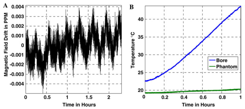
a Frequency measurement variation when the magnet system is thermally stable on the 1.5 T GE system, showing the stability and accuracy of measurements. The periodic nature is attributable to the air conditioning cycle in the electronics room. b Curve showing the temperature rise inside the bore of the MR scanner while an SSFP sequence is running

Fig. 2.

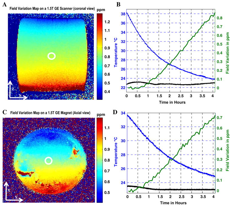
a Magnetic field changes in the x–z (coronal) plane after 4 h on a 1.5 T GE system. b Curves of the temporal field variation in the iso-center of the magnet (green), temperature temporal variation at the bore of the magnet (blue) and in the phantom (black). c Magnetic field changes in the x–y (axial) plane after 4 h on a 1.5 T GE system. The spatial nonlinearity results from voids in the phantom. d Curves of the temporal field variation in the iso-center of the magnet (green), temperature temporal variation at the bore of the magnet (blue) and in the phantom (black)

Table 1.

Fitted field coefficients of the quadratic model for the three scanners

GE field monitoring
[Coronal]	α0	αi t z	αx	αz2	αx2	αzx
Values	0.85 ppm	−2.8 ppm/m	0.13 ppm/m	1.0 ppm/m2	3.0 ppm/m2	−1.0 ppm/m2
[Axial]	α0	αy	αx	αy2	αx2	αyx
Values	0.71 ppm	−4.4 ppm/m	0.22 ppm/m	2.0 ppm/m2	1.6 ppm/m2	−2.0 ppm/m2
Philips field monitoring
[Coronal]	α0	αz	αx	αz2	αx2	αzx
Value	2.02 ppm	−1.8 ppm/m	0.33 ppm/m	5.0 ppm/m2	−4.0 ppm/m2	−1.0 ppm/m2
Value [45°]	2.19 ppm	−2.3 ppm/m	0.3 ppm/m	7.0 ppm/m2	−4.0 ppm/m2	−1.0 ppm/m2
[Axial]	α0	αy	αx	αy2	αx2	αyx
Value	0.8 ppm	−0.38 ppm/m	0.53 ppm/m	0.2 ppm/m2	0.5 ppm/m2	0.9 ppm/m2
Siemens field monitoring
[Coronal]	α0	αz	αx	αz2	αx2	αyx
Value	−0.3 ppm	0.41 ppm/m	0.19 ppm/m	10.0 ppm/m2	−2 ppm/m2	−0.1 ppm/m2
MR thermometry (Philips scanner)
[Axial]	α0	αy	αx	αy2	αx2	αyx
Value	−0.43 ppm	−0.42 ppm/m	−0.15 ppm/m	1.3 ppm/m2	1.18 ppm/m2	1.17 ppm/m2
Value	2.43 ppm	−0.04 ppm/m	−1.16 ppm/m	1.15 ppm/m2	−0.5 ppm/m2	0.15 ppm/m2

GE field monitoring. Upper row: estimated parameters of the spatial quadratic fit to the field variation map using 10 K points with an accuracy of fit of 0.012 ppm; coronal plane. Lower row: estimated parameters of the spatial quadratic fit to the field variation map using 10 K points with an accuracy of fit of 0.016 ppm; axial plane

Philips field monitoring [Coronal]. Upper row, estimated parameters of the spatial quadratic fit to the field variation map using 10 K points with an accuracy of fit of 0.011 ppm. Lower row, estimated parameters of the spatial quadratic fit to the field variation map using 10 K points with an accuracy of fit of 0.013 ppm; coronal plane rotated by 45°

Philips field monitoring [Axial]. Estimated parameters of the spatial quadratic fit to the field variation map using 5 K points with an accuracy of fit of 0.006 ppm

Siemens field monitoring. Estimated parameters of the spatial quadratic fit to the field variation map using 5 K points with an accuracy of fit of 0.007 ppm; coronal plane. Field variation has both linear and quadratic terms in the z direction and a linear component in the y direction

MR Thermometry. Upper row: estimated parameters for Fig. 6a of the spatial phase quadratic fit over the reference phantom showing the need for multiple non-collinear references to correct for field variation terms. Lower row: estimated parameters for Fig. 7a of the spatial phase quadratic fit over the reference phantom showing a heavily weighted linear x term. The baseline phase variation pattern is different from that obtained from MR thermometry experiment started when the scanner was in an initial stable condition

Philips experiments

Measurements from temperature probes located in the phantom, the bore of the magnet, and on the copper nut on the gradient cooling outflow are plotted in Fig. 3a as the SSFP sequence was running. Figure 3c illustrates temperature probes readings as a function of time after SSFP ended and as the field was monitored. Figure 3b shows the field variation in the x–z plane using PDI (method B) and an SPGR sequence. Figure 3d is the result for the experiment with the coronal plane rotated 45° and the z-gradient turned on. The magnitudes of the spatial field variations are comparable to those obtained from the GE scanner (Table 1).

Fig. 3.

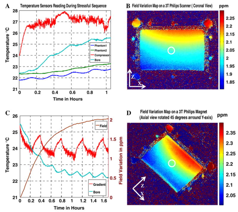
a Dark blue and green curves are temporal temperature fiberoptic probe readings of the phantom during an SSFP stressful sequence running on the 3 T Philips scanner. Light-blue curve is the temperature at surface of the bore of the magnet and the red curve is the reading from the probe stuck on the surface of the copper washer connecting the outflow water hose from the gradient cooling housing to the heat exchange compressor. b Magnetic field changes in the x–z (coronal) plane after 1.65 h on the 3 T Philips system. c The brown curve is the temporal field variation at the iso-center of the magnet and the rest of the curves represent temperature probe readings as explained in part (a) during the cooling process of the magnet. It is noted that the temperature of the gradient cooling system cycles representing the normal periodic operation of the cooling compressor. d Magnetic field changes in the x–z (coronal) plane rotated by 45° after 2.25 h of cooling on the 3 T Philips system

Variations of this experiment performed with the shim gradients turned off and using B₀ mapping (method A) and PDI (method B), yielded the same results, excluding the possibility that the observed effects result from the system gradients or shim gradients directly. Figure 4 depicts the results of axial field monitoring using a SPGR sequence with two different echo times. Both x and y field variations are evident (Table 1). Experiments repeated using PDI, with and without the shim gradients, yielded the same results. The stabilization time for the Philips scanner following the SSFP stress is of the order of 2–3 h, but this system is new and its cooling/ventilation system is more efficient.

Fig. 4.

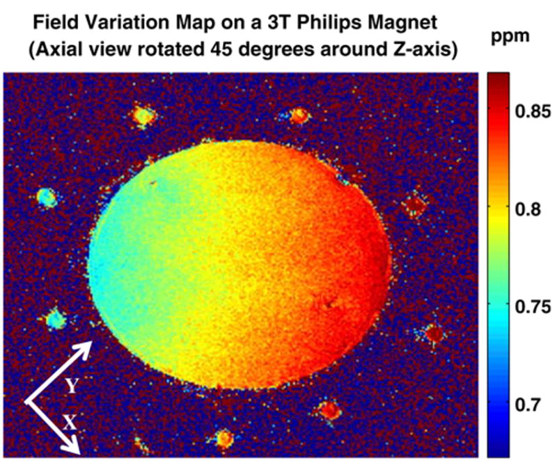
Magnetic field changes in the x–y (axial) plane rotated by 45° after 1.4 h (cooling time) on the 3 T Philips system

Siemens experiment

Figure 5 shows the coronal field variation after 1.7 h of cooling on the Siemens system. Again, both temporal and spatial variations are evident (Table 1).

Fig. 5.

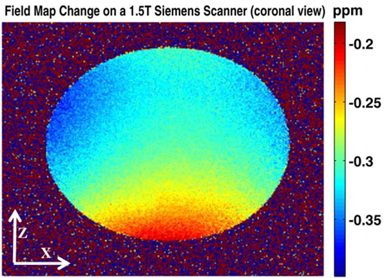
Magnetic field changes in the x–z (coronal) plane after 1.7 h since cooling started on the 1.5 T Siemens system

Temperature monitoring experiments

Figure 6a shows the field variation at the end of the 40 min initial temperature monitoring sequence. Resultant phase changes due to spatial field variation completely masks the phase variations due to the local heating source (Table 1). The corrected temperature maps are shown in Fig. 6b. The estimated temperature temporal curve using MR thermometry is in close agreement with the fiber-optic sensor at the point where local heating was applied (Fig. 6c).

Fig. 6.

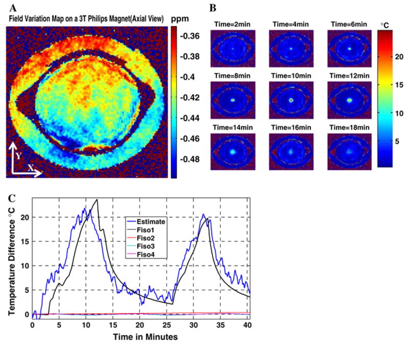
a Magnetic field changes in the x–y (axial) plane at the end of the MR thermometry experiment on the 3 T Philips system (magnet is in an initial thermal stable condition). Temperature information is totally masked by field variation effects. b Temperature maps at different time instances after the correction of magnetic field changes. c The dark-blue curve is the temporal temperature estimate using corrected MR thermometry at the point where a fiber-optic temperature sensor is inserted in the gel phantom. A total average estimation error of 2.5 °C is calculated. The other three curves are control sensor reading placed in the gel phantom and on the reference showing no significant heating generated by the MR pulse sequence

The second experiment is conducted after the scanner is thermally disturbed by a 30 min SSFP sequence. Figure 7 shows the spatial field variation at the end of the temperature monitoring sequence, along with the temperature maps/curves obtained after referenced correction. The zero-order field variation term (Table 1) indicates that the scanner’s field is drifting in the opposite direction compared to the earlier experiment. The reason is that the scanner is now cooling and the sequence used to monitor temperature does not generate enough energy to heat the scanner or maintain its thermal stability. The calculated σ (ΔB₀) for the experiment is 0.032 ppm corresponding to a temperature estimation uncertainty of 3.2 °C. The high estimation uncertainty is attributable to the short TE used to avoid phase wraps and results in the imperfect temperature detection, as suggested by both Figs. 6c and 7c.

Fig. 7.

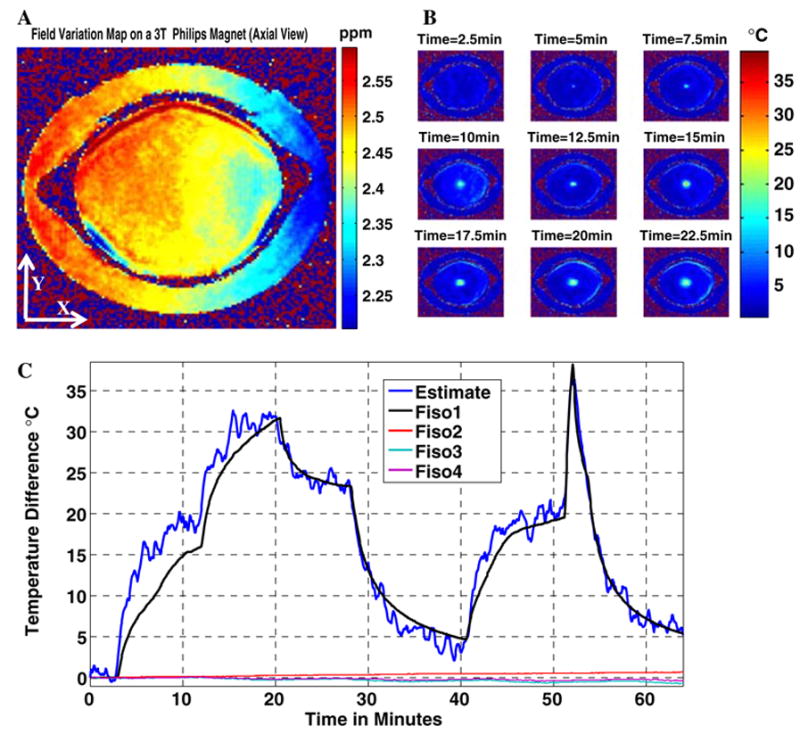
a Magnetic field changes in the x–y (axial) plane at the end of the MR thermometry experiment on the 3 T Philips system (magnet is in an initial thermal instability condition after being perturbed with a 30 min SSFP sequence). Temperature information is totally masked by field variation effects. b Temperature maps at different time instances after the correction of magnetic field changes. c Dark blue curve is the temporal temperature estimate using corrected MR thermometry at the point where a fiber-optic temperature sensor is inserted in the gel phantom. A total average estimation error of 1.7 °C is calculated. The other three curves are control sensor reading placed in the gel phantom and on the reference showing no significant heating generated by the MR pulse sequence

Spectroscopy experiments

The ¹H spectroscopy experiment on the phantom shows that after the scanner is thermally perturbed by repeatedly exercising the MR gradients, the water resonance is broadened and the field homogeneity degraded (Fig. 8). This result demonstrates the need for online field corrections for localized spectroscopy following gradient stress during the course of a study. Table 2 quantifies parametrically the loss in field homogeneity. Gradient shimming partially compensated for the degradation, as shown in Table 3.

Fig. 8.

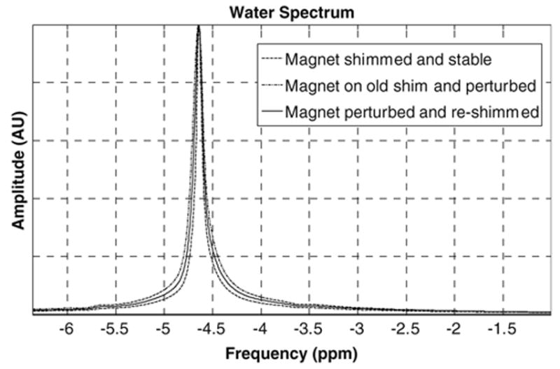
The spectrum acquired over a 13.5 cm³ voxel from the saline spherical phantom at the iso-center of the magnet. Effect of field homogeneity change is shown as a FWHM spectral broadening of the water peak from 8.5 to 18.5 Hz and then to 12.5 Hz after field homogeneity correction

Table 2.

Model field parameters for spectroscopy experiments

F0 (ppm)	Gx (ppm/m)	Gy (ppm/m)	Gz (ppm/mm)	Gx2y2 (ppm/m2)	G2xy (ppm/m2)	Gzy (ppm/m2)	Gzx (ppm/m2)	Gz2 (ppm/m2)
Phantom
0.625	0.73	−1.23	−1.8	3.46	−0.5	−18.83	2.46	19.2
Human brain study
2	0.333	0.2	−1.46	2.1	−4.73	17.4	−3.96	18

Phantom study: 3D quadratic spatial model parameters of the field variation map.

Human brain study: 3D quadratic spatial model parameters of the field variation map

Table 3.

Frequency variation (SD) and line width over spectroscopy voxels

Phantom			Brain study
	B0-maps SD (Hz)	Water line width (Hz)	B0-maps SD(Hz)	NAA line width (Hz)
Before	6	8.5	6	5.5
After	13	18.5	11.7	20
Corrected	8	12.5	8	10

Phantom study: calculated frequency STD over the region used to acquire ¹H spectra.

Brain study: calculated frequency STD over the region used to acquire ¹H spectra

The results of the in vivo study are shown in Fig. 9. Figure 9a shows the anatomical image and selected voxel, and Fig. 9b shows the corresponding initial spectrum. Figure 9c shows the degradation in both peak width and SNR as the field varies after 30 min of EPI. Fig. 9d was acquired after the field was re-shimmed at this point, showing partial, albeit incomplete, restoration of the SNR and reduction in line width. Table 2 parametrically documents the loss in field homogeneity, and Table 3 illustrates both the degradation in field homogeneity and the extent to which it is compensated by re-shimming.

Fig. 9.

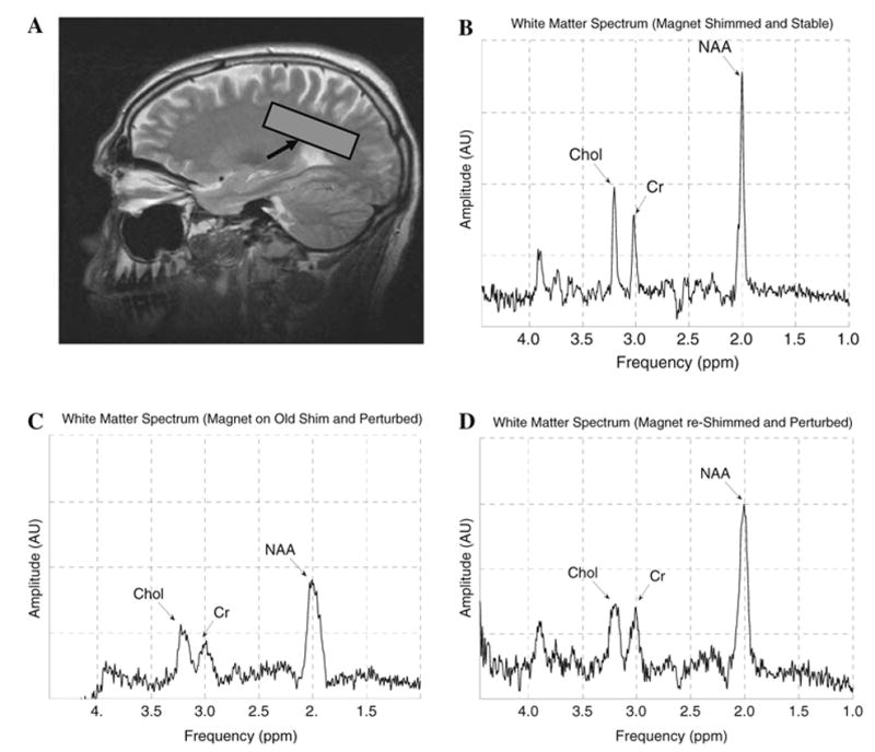
a A turbo spin-echo (TSE) sagittal high-resolution image showing the location where the spectra of the brain white matter is acquired. b The acquired spectrum of the brain when the magnet is in a stable condition. NAA FWHM is 5.5 Hz. The Choline (Chol) and Creatine (Cr) peaks are well resolved. c The spectrum of the brain after the magnetic field varied due to a 30 min functional scan. The decrease in the field homogeneity causes the NAA FWHM to increase to 20 Hz. The Chol and Cr peaks are now smeared. d The brain spectrum is improved by re-shimming the field and drift correction. Now NAA FWHM is 10 Hz and the resolution between the Chol and Cr peaks is improved

Discussion and Conclusion

Experiments conducted here demonstrate that continuous, prolonged gradient use alters the stability and homogeneity of the main magnetic field of horizontal bore 1.5 T and 3 T clinical MR scanners. In all of the field-monitoring experiments, the observed fluctuations in ppm were two orders of magnitude greater than the experimental uncertainty, and deviations from the quadratic model used for fitting the field were less than 1% of the true, MRI-determined, field inhomogeneity. The effects are time dependent and are of sufficient magnitude to obfuscate PRF MR thermometry measurements and to significantly degrade in vivo MR spectroscopy performance. The findings implicate heating of the magnet bore generated by the MRI gradient system (from Joule heating and/or eddy-current losses) as the culprit. Although the temperature sensors inside the MR scanner were limited by accessibility to locations away from the likely sites of heating, they nevertheless provide evidence of thermal perturbation. The phase difference techniques used to monitor the field are not affected by changes in gradients that may result from variations in gradient eddy current compensation, as evidenced by experiments on the Philips scanner which documented the same spatiotemporal field variations with the active shimming gradients turned off. In addition, such variations would result in image deformation that was not noticed during these studies. Although a different phantom and T/R coil were used for the Siemens studies, because the measurements are of MRI frequency differences which are independent of the material properties given that the sample temperature is constant over the period of each study, changing the phantom has no effect on the findings.

A main cause of the observed temporal and spatial variations in field homogeneity may lie with the passive shims. Passive shimming utilizes small ferromagnetic materials distributed cylindrically in a grid between the gradients and the magnet’s bore, as magnetic dipoles to correct main magnetic field inhomogeneity. Switching the MRI system’s gradients induces eddy currents in the resistive iron shims, which heats them [18]. Because the magnetic susceptibility of the material is both temperature dependent and has a high thermal expansion coefficient, temperature variations can affect the spatial distribution of the passive correction field. The assumption of a constant field drift [3,19] is only true as a first order approximation and is evidently inadequate to explain the behavior demonstrated in this study. A possible solution for the manufacturers would be to regulate the temperature of the passive shims by including them in the cooling mechanisms of the magnet’s bore or gradient coils. Recent patents [20–22] suggest various cooling mechanisms to regulate field changes due to the magnetic properties of ferromagnetic shims. Until this problem is solved with MRI scanner design modifications, both spatial and temporal field variations will occur with studies using gradient-demanding MR pulse sequences.

An important aspect of the findings is that the time-constants for these variations differ from scanner to scanner, and with the intensity and duration of the sequences being applied. Thus, an 8-year-old GE scanner did not reach thermal stability after more than 4 h, while a new Philips system stabilized in 2–3 h. The aim of the current study is not to compare the thermal stability of different manufacturer’s scanners, but rather to demonstrate that this problem is prevalent on scanners produced by the three most common vendors. Consequently, special attention is warranted during MR procedures that are sensitive to phase variations, even when the scan itself is not gradient-intensive, because the scanner may be in a thermally unstable condition due to a previous scan. Clearly, this would include MR-guided interventional hyper- or hypotherapy procedures in patients where MR thermometry is used for monitoring.

Analysis of the spatial field variations indicates the presence of quadratic terms, especially in the z direction. Therefore, for phase-sensitive MR procedures performed under the conditions described, it is necessary to use spatially varying field-compensation strategies. The need to adopt referenced field-correction methods using quadratic polynomial models is demonstrated here for PRF thermometry. The assumption of a linear model adopted previously [23] is less accurate, especially for coronal planes. Alternative methods of correcting field variations during MR thermometry include use of referenceless techniques that use phase information far from the sites where local temperature is being monitored [17,24,25].

Similarly, it is often assumed that only uniform field drifts need be corrected during prolonged exams involving MR spectroscopy. Because the scanner magnetic field homogeneity may change with time, our study demonstrates that re-shimming is needed, especially when the spectroscopy study is combined or interleaved with gradient-intensive functional-MRI-type acquisitions. Re-shimming was able to partially compensate for field homogeneity variations in our phantom and human experiments.

Other MR experiments sensitive to, or that utilize phase measurements such as flow and velocity mapping sequences may also be susceptible to field variations wrought by prolonged SSFP, or fMRI/EPI-based pulse sequences [6,26]. Since the scanner heats up during daily procedures the status of the magnetic field will in general depend on the time of day, and its recent utilization history. Until a physical solution is developed a scanner’s field variations may require characterization with well-understood settling times, in order to optimize performance for phase-sensitive applications. Meanwhile, interleaving fast field-mapping methods [27,28] during existing MR sequences is probably the best method to account for, and compensate for, such field variations.

Finally, while our study was limited to three scanners, that magnetic field variations of comparable magnitude were seen in all three scanners produced by three different manufacturers, suggests that the problem is endemic. Recognizing and understanding the nature of the field variations, we think, represents a significant step toward developing solutions that improve the accuracy, utility, and indeed viability, of phase-sensitive MR.

References

- 1.Barkauskas KJ, Lewin JS, Duerk JL. Variation correction algorithm: analysis of phase suppression and thermal profile fidelity for proton resonance frequency magnetic resonance thermometry at 0.2 T. J Magn Reson Imaging. 2003;17(2):227–240. doi: 10.1002/jmri.10239. [DOI] [PubMed] [Google Scholar]
- 2.Peters RD, Hinks RS, Henkelman RM. Ex vivo tissue-type independence in proton-resonance frequency shift MR thermometry. Magn Reson Med. 1998;40(3):454–459. doi: 10.1002/mrm.1910400316. [DOI] [PubMed] [Google Scholar]
- 3.Henry PG, van de Moortele PF, Giacomini E, Nauerth A, Bloch G. Field-frequency locked in vivo proton MRS on a whole-body spectrometer. Magn Reson Med. 1999;42(4):636–642. doi: 10.1002/(sici)1522-2594(199910)42:4<636::aid-mrm4>3.0.co;2-i. [DOI] [PubMed] [Google Scholar]
- 4.De Poorter J. Noninvasive MRI thermometry with the proton resonance frequency method: study of susceptibility effects. Magn Reson Med. 1995;34(3):359–367. doi: 10.1002/mrm.1910340313. [DOI] [PubMed] [Google Scholar]
- 5.Haacke EM, Brown RW, Thompson M, Venkatesan R. Magnetic resonance imaging: Principles and sequence design. Wiley; New York: 1999. pp. 746–760. [Google Scholar]
- 6.Kadah YM, Hu X. Simulated phase evolution rewinding (SPHERE): a technique for reducing B0 inhomogeneity effects in MR images. Magn Reson Med. 1997;38(4):615–627. doi: 10.1002/mrm.1910380416. [DOI] [PubMed] [Google Scholar]
- 7.Ishihara Y, Calderon A, Watanabe H, Okamoto K, Suzuki Y, Kuroda K, Suzuki Y. A precise and fast temperature mapping using water proton chemical shift. Magn Reson Med. 1995;34(6):814–823. doi: 10.1002/mrm.1910340606. [DOI] [PubMed] [Google Scholar]
- 8.Irarrazabal P, Meyer CH, Nishimura DG, Macovski A. Inhomogeneity correction using an estimated linear field map. Magn Reson Med. 1996;35(2):278–282. doi: 10.1002/mrm.1910350221. [DOI] [PubMed] [Google Scholar]
- 9.Quesson B, de Zwart JA, Moonen CT. Magnetic resonance temperature imaging for guidance of thermotherapy. J Magn Reson Imaging. 2000;12(4):525–533. doi: 10.1002/1522-2586(200010)12:4<525::aid-jmri3>3.0.co;2-v. [DOI] [PubMed] [Google Scholar]
- 10.Peters RD, Henkelman RM. Proton-resonance frequency shift MR thermometry is affected by changes in the electrical conductivity of tissue. Magn Reson Med. 2000;43(1):62–71. doi: 10.1002/(sici)1522-2594(200001)43:1<62::aid-mrm8>3.0.co;2-1. [DOI] [PubMed] [Google Scholar]
- 11.Kanayama S, Kuhara S, Satoh K. In vivo rapid magnetic field measurement and shimming using single scan differential phase mapping. Magn Reson Med. 1996;36(4):637–642. doi: 10.1002/mrm.1910360421. [DOI] [PubMed] [Google Scholar]
- 12.David F, Yerucham S. InSightec —TxSonics Ltd. (Tirat Carmel, IL) assignee (2003) MRI-based temperature mapping with error compensation. 6,559,644. USA Patent. 2003 May 6;
- 13.Bottomley PA. Spatial localization in NMR spectroscopy in vivo. Ann N Y Acad Sci. 1987;508:333–348. doi: 10.1111/j.1749-6632.1987.tb32915.x. [DOI] [PubMed] [Google Scholar]
- 14.Schar M, Kozerke S, Fischer SE, Boesiger P. Cardiac SSFP imaging at 3 Tesla. Magn Reson Med. 2004;51(4):799–806. doi: 10.1002/mrm.20024. [DOI] [PubMed] [Google Scholar]
- 15.Gabr RE, Sathyanarayana S, Schär M, Weiss RG, Bottomley PA. On restoring motion-induced signal loss in single-voxel magnetic resonance spectra. Magn Reson Med. 2006;56(4):757–760. doi: 10.1002/mrm.21015. [DOI] [PMC free article] [PubMed] [Google Scholar]
- 16.de Zwart JA, Vimeux FC, Delalande C, Canioni P, Moonen CT. Fast lipid-suppressed MR temperature mapping with echo-shifted gradient-echo imaging and spectral–spatial excitation. Magn Reson Med. 1999;42(1):53–59. doi: 10.1002/(sici)1522-2594(199907)42:1<53::aid-mrm9>3.0.co;2-s. [DOI] [PubMed] [Google Scholar]
- 17.Rieke V, Vigen KK, Sommer G, Daniel BL, Pauly JM, Butts K. Referenceless PRF shift thermometry. Magn Reson Med. 2004;51(6):1223–1231. doi: 10.1002/mrm.20090. [DOI] [PubMed] [Google Scholar]
- 18.Silva AC, Merkle H. Hardware considerations for functional magnetic resonance imaging. Conc Magn Res. 2003;16A(1):35–49. [Google Scholar]
- 19.Foerster BU, Tomasi D, Caparelli EC. Magnetic field shift due to mechanical vibration in functional magnetic resonance imaging. Magn Reson Med. 2005;54(5):1261–1267. doi: 10.1002/mrm.20695. [DOI] [PMC free article] [PubMed] [Google Scholar]
- 20.Emeric PR, Hedlund CR. GE Electric Company, Schenectady, NY (US), assignee (2006). Method and system to regulate cooling of a medical imaging device. 6,992,483, B1. US patent. 2006 January 31;
- 21.Clarke N, Sellers MB, Allford ML, Mantone A. GE Electric Company, Schenectady, NY (US), assignee (2006) Apparatus for active cooling of an MRI patient bore in cylindrical MRI systems. 7,015,692. US Patent. 2006 March 21;
- 22.Gebhardt M, Gebhardt N, Schuster J. Siemens Aktiengesellschaft, Munich (DE), assignee (2005) Magnetic resonance apparatus and carrier device equipable with shim elements. 6,867,592. US Patent. 2005 Mar 15;
- 23.Behina B, Suthar M, Webb AG. Closed-loop feedback control of phased-array microwave heating using thermal measurements from magnetic resonance imaging. Conc Magn Res. 2002;15(1):101–110. [Google Scholar]
- 24.Rieke V, Vigen KK, Sommer G, Diederich CJ, Nau WH, Ross A, Daniel BL, Pauly JM, Butts K. Referenceless PRF shift thermometry. ISMRM; Canada: 2003. [DOI] [PubMed] [Google Scholar]
- 25.Schneider E, Cline E, Washburn S, Hardy CJ. General Electric Company, Wausksha, WI, assignee (1998) Real time in vivo measurement of temperature changes with NMR imaging. 5,711,300. US Patent. 1998 Jan 27;
- 26.Jezzard P, Clare S. Sources of distortion in functional MRI data. Hum Brain Mapp. 1998;8(2–3):80–85. doi: 10.1002/(SICI)1097-0193(1999)8:2/3<80::AID-HBM2>3.0.CO;2-C. [DOI] [PMC free article] [PubMed] [Google Scholar]
- 27.Santos JM, Cunningham CH, Lustig M, Hargreaves BA, Hu BS, Nishimura DG, Pauly JM. Single breath-hold whole-heart MRA using variable-density spirals at 3T. Magn Reson Med. 2006;55(2):371–379. doi: 10.1002/mrm.20765. [DOI] [PubMed] [Google Scholar]
- 28.Roopchansingh V, Cox RW, Jesmanowicz A, Ward BD, Hyde JS. Single-shot magnetic field mapping embedded in echo-planar time-course imaging. Magn Reson Med. 2003;50(4):839–843. doi: 10.1002/mrm.10587. [DOI] [PubMed] [Google Scholar]