Auditory Cortical Responses Elicited in Awake Primates by Random Spectrum Stimuli

Abstract

Contrary to findings in subcortical auditory nuclei, auditory cortex neurons have traditionally been described as spiking only at the onsets of simple sounds such as pure tones or bandpass noise and to acoustic transients in complex sounds. Furthermore, primary auditory cortex (A1) has traditionally been described as mostly tone responsive and the lateral belt area of primates as mostly noise responsive. The present study was designed to unify the study of these two cortical areas using random spectrum stimuli (RSS), a new class of parametric, wideband, stationary acoustic stimuli. We found that 60% of all neurons encountered in A1 and the lateral belt of awake marmoset monkeys (Callithrix jacchus) showed significant changes in firing rates in response to RSS. Of these, 89% showed sustained spiking in response to one or more individual RSS, a substantially greater percentage than would be expected from traditional studies, indicating that RSS are well suited for studying these two cortical areas. When firing rates elicited by RSS were used to construct linear estimates of frequency tuning for these sustained responders, the shape of the estimate function remained relatively constant throughout the stimulus interval and across the stimulus properties of mean sound level, spectral density, and spectral contrast. This finding indicates that frequency tuning computed from RSS reflects a robust estimate of the actual tuning of a neuron. Use of this estimate to predict rate responses to other RSS, however, yielded poor results, implying that auditory cortex neurons integrate information across frequency nonlinearly. No systematic difference in prediction quality between A1 and the lateral belt could be detected.

Introduction

Characteristics of auditory cortex neurons have remained relatively elusive despite numerous experimental inquiries. Even a fairly straightforward property such as mapping of characteristic frequency (CF) was clarified sufficiently only after decades of research (Woolsey and Walzl, 1942; Evans et al., 1965; Goldstein et al., 1970; Merzenich et al., 1973; Goldstein and Abeles, 1975b; Merzenich et al., 1975). A large portion of this problem undoubtedly arises from the difficulty in finding classes of acoustic stimuli capable of eliciting significant spiking discharges from many cortical neurons. The auditory cortex literature, for example, contains many accounts of neurons found to spike only at the onset of unmodulated acoustic stimuli, if at all (Erulkar et al., 1956; Brugge et al., 1969; Abeles and Goldstein, 1970, 1972; Miller et al., 1980; Phillips et al., 1996; Eggermont, 1997; Heil, 1997a,b; Furukawa et al., 2000). Such onset-only responses tend to reflect spiking behavior that locks to the envelope of a stimulus (“phasic”) rather than persisting throughout the stimulus interval in a sustained, nonsynchronized manner (“tonic”). Phasic auditory cortex neurons have been widely reported enough to fuel speculation that the auditory cortex is predominantly an encoder of acoustic transients (Schreiner and Urbas, 1986; Phillips, 1988; Phillips and Sark, 1991; Heil, 1997a,b; Poldrack et al., 2001).

Stimuli most commonly used to study the auditory cortex of nonspecialized mammals include the familiar clicks, tones, and bandpass noise (possibly repeated, modulated, in various combinations, or from various spatial directions) plus animal vocalizations (Rauschecker et al., 1995; Wang et al., 1995) and spectro-temporally complex parametric wideband stimuli (Schreiner and Calhoun, 1994; Shamma et al., 1995; Kowalski et al., 1996; deCharms et al., 1998; Versnel and Shamma, 1998; Klein et al., 2000; Depireux et al., 2001; Schnupp et al., 2001; Miller et al., 2002). In general, findings from experiments using these stimulus protocols in auditory cortex appear to substantiate the classical assertions that most cortical neurons tend to respond in a phasic manner. Recent studies in awake marmoset monkeys, however, have revealed that tonic responses in auditory cortex may be more common than previously believed (Wang et al., 2002; Barbour and Wang, 2003), although these observations are not strictly novel (Brugge and Merzenich, 1973; Goldstein and Abeles, 1975a; Shamma et al., 1993; Recanzone, 2000). Indeed, neurons with nonsynchronized spiking behavior appear to represent an important class of stimulus encoding in auditory cortex (Lu et al., 2001).

Parametric, wideband, stationary acoustic stimuli have been used to characterize the rate coding of neurons in subcortical auditory centers with great success (Calhoun et al., 1998; Yu and Young, 2000, 2002). These recent results have confirmed earlier findings and improved understanding of the rate coding of several classes of neurons. The present study was undertaken to evaluate the hypothesis that experimental and stimulus design can reveal stimulus-invariant spectral tuning properties of auditory cortex neurons as measured by a rate code.

Materials and Methods

Physiological recordings and acoustic stimulus delivery. Marmoset monkeys (Callithrix jacchus) were prepared for data collection following institution-approved chronic physiology procedures (Barbour and Wang, 2002). Extracellular tungsten microelectrodes (3-5MΩ at 1 kHz) (A-M Systems) were lowered through microcraniotomies in the skull (<1 mm diameter), allowing stable recordings of well isolated single units [>40 dB waveform signal-to-noise ratio (SNR) possible; typical SNR >30 dB] for many hours. Action potential waveforms were monitored continuously during each recording session and sorted on-line by template-matching digital signal processing software (Alpha-Omega Engineering). Spike timing information was passed through event timing equipment (Tucker Davis Technologies) and logged using custom software running on a Pentium-based personal computer. Units were sampled from all cortical layers and often from supragranular layers. Primary auditory cortex (A1) was located stereotactically and confirmed by its short-latency, tone-responsive units and its tonotopic map. When all desired physiological experiments for an animal had been conducted, electrolytic lesions and fluorescent dye injections were made at sites in and around primary auditory cortex. The animal was then deeply anesthetized with Nembutal, killed, and perfused with formalin to preserve the brain tissue. Serial sectioning and staining revealed the precise locations of the lesions and injections, which when combined with the experimental record can be used to pinpoint the recording sites.

Custom software running in MatLab generated all sound stimuli digitally at 100,000 samples per second at full 16 bit dynamic range. The signals were converted to analog, filtered, and attenuated (0 dB attenuation equals ∼93 dB sound pressure level @ 1 kHz) before being passed into the acoustic recording chamber (IAC-1024, Industrial Acoustics Company), the interior of which was lined with 3 inch acoustic foam (Sonex, Illbruck). All of the stimuli were delivered in free field through a single two-way crossover, open bass reflex loudspeaker (B&W 601) located 70 cm in front of the animal's head and calibrated using a Brüel and Kjær condenser microphone in place of the animal's head. All stimuli were presented pseudorandomly for 5 or 10 repetitions. Spontaneous activity was estimated from neuronal spiking during the silent periods preceding the stimuli. Stimuli were always separated by ≥1 sec of silence.

Random spectrum stimulus generation. Acoustic stimuli used for these experiments were adapted from similar stimuli devised by E. D. Young (Johns Hopkins University School of Medicine) to study subcortical auditory neurons (Yu and Young, 2000). These random spectrum stimuli (RSS) contain many simultaneous pure tones spaced logarithmically in carrier frequency with randomized sound levels. The tones are grouped into equal-width frequency bins such that all tones falling within one bin share an identical sound level. This arrangement allows the spectral profile to be varied independently from the frequency distribution of the tones. Independent RSS parameters for these experiments consisted of stimulus duration, linear ramp duration, carrier frequency range (i.e., bandwidth), bin density, mean sound level, tone density, and bin levels (i.e., spectral profile). RSS were constructed on-line with durations of ≥100 msec. Ramp duration was fixed at 10 msec onset and offset. Bin densities were generally 20 bins per octave, although an occasional narrowly tuned unit required a bin density of 40 bins per octave for adequate characterization. Stimulus bandwidths ranged from two to four octaves, and overall frequency range was adjusted as needed to include a unit's CF. Bin levels were randomized. Mean level, tone density, and bin level SD were varied systematically or adjusted by hand as appropriate for each unit. Several representations of two example RSS from one set are shown in Figure 1.

Figure 1.

Example random spectrum stimuli (RSS) from the same set. Two RSS from the same stimulus set are shown plotted as bin levels (top), tone levels (middle), and amplitude spectra (bottom). The bins have a level SD of 10 dB over the entire set, indicated by horizontal dotted lines. All of the stimuli span two octaves of frequency from 4 to 16 kHz with 20 bins per octave. Each bin contains three logarithmically spaced tones of the same level for a density of 60 tones per octave. This set contained an additional 41 stimuli, including the stimulus with all bin levels at the mean value (i.e., the flat-spectrum stimulus).

A row vector of sound levels reflecting the spectral profile, when coupled with scalar values accounting for all other parameters, can uniquely represent any individual RSS. If the mean sound level is subtracted from all bins of the level vector, the zero-mean adjusted level vector results: . These adjusted level vectors are depicted graphically in Figure 1 (top panels). RSS are designed in sets of stimuli having identical parameters except for the spectral profiles; these sets can be represented by collecting the adjusted level row vectors into an adjusted level matrix Λ. The adjusted level matrix has rows indexed by stimulus number and columns indexed by frequency bin, as can be seen in Figure 2 A.

Figure 2.

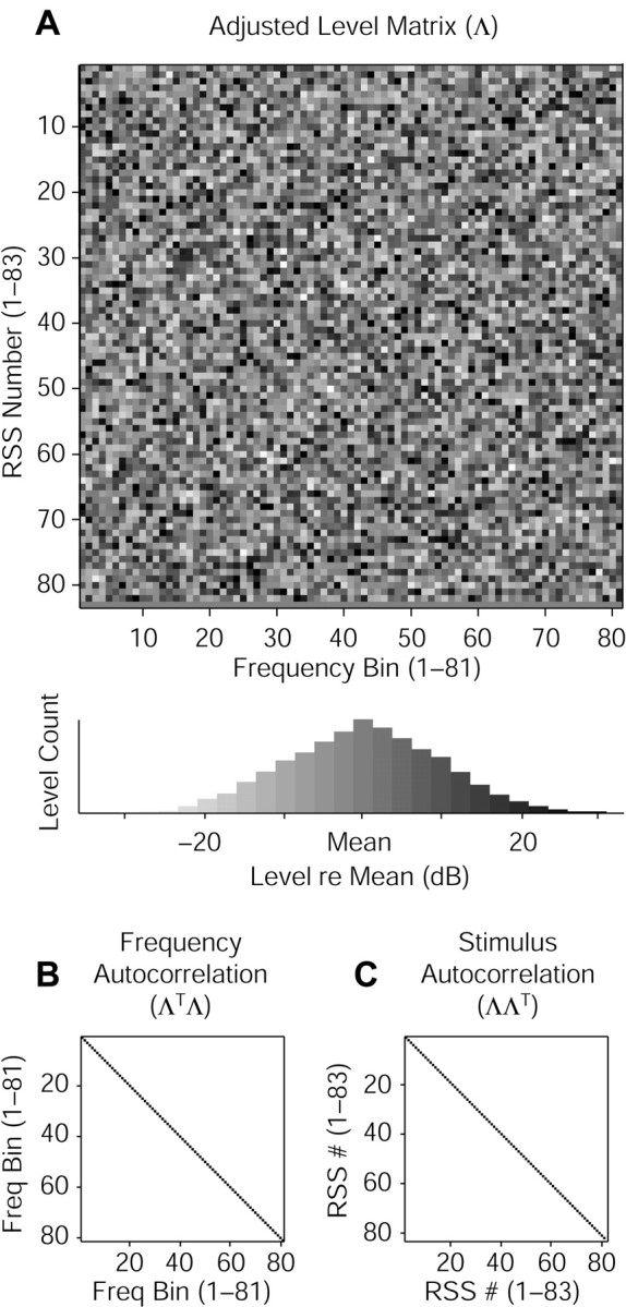
Graphic depiction of RSS set properties. A, An adjusted level matrix (Λ) is shown in levels of gray. Individual stimuli are plotted in rows; frequency bins are plotted in columns. The matrix has 81 bins, each with a normal level distribution (histogram below) of 10 dB SD, and 83 stimuli, with the flat-spectrum stimulus represented in the bottom row. This matrix was used to create a stimulus four octaves wide (2-32 kHz) with 20 bins per octave, which was then used to characterize the unit shown in Figure 3. B, Autocorrelation of the adjusted level matrix columns (Λ^TΛ) indicates an orthonormal column space. C, Autocorrelation of the rows (ΛΛ^T) indicates white (uncorrelated) stimuli.

An RSS set represents a collection of stimulus vectors sampling the space of all possible stationary (i.e., non-time varying) spectral profiles at the resolution of the bin density. For weighting functions (defined below) to achieve optimal linear estimates of tuning, two constraints must be placed on the adjusted level matrix. First, the basis set for the stimuli must have linearly independent elements. The frequency bins constitute the basis set for RSS; because they do not overlap, they are mutually orthogonal and therefore independent. The adjusted level matrix reflects this orthogonality in its column space: its frequency autocorrelation matrix should factor into a scalar multiplied by the identity matrix, as shown in Figure 2 B: Λ^TΛ + ϵ_Λ^T_ΛI.

Second, the stimuli must uniformly and randomly sample the stimulus space. This constraint is realized if the stimulus vectors are randomly oriented, of equal norm, and maximally dispersed in the space (i.e., any pair of stimulus vectors share the same inner product). Correspondingly, the stimulus autocorrelation matrix should factor into a scalar multiplied by the identity matrix, as shown in Figure 2C: ΛΛ^T = ϵ_ΛΛ^TI. This constraint yields columns of Λ that have means of 0; consequently, where is any column vector of constants.

These two constraints can be met simultaneously only for rectangular adjusted level matrices having more rows than columns. Additionally, the central limit theorem guarantees that the sound level distribution in each frequency bin will tend toward a normal distribution, thereby yielding the familiar white, Gaussian stimulus set traditionally associated with optimal linear estimates (de Boer and Kuyper, 1968; de Boer and de Jongh, 1978; Aertsen and Johannesma, 1981; Theunissen et al., 2000). Naturally, cortical rate codes in response to stationary stimuli must exist for the preceding derivation to prove useful.

Construction of linear spectral weighting functions. The RSS described above can be used to build a model of how an auditory cortex neuron where k responds to stationary stimuli having arbitrary spectra. A linear model for such a case can be written as:

1

where _lin is a column vector of m rate values predicted in response to the set of m different RSS, is a constant column vector of m identical rate values predicted in response to a single RSS with all bin levels set to the mean sound level, Λ is the m × n adjusted level matrix, and is a column vector of n values representing the linear spectral weighting function (WF). The numbers of stimuli and frequency bins are indicated by m and n, respectively. All rates here are “driven rates” (discharge rate minus spontaneous rate) so that negative values indicate suppression. Equation 1 is referred to as the model equation or linear synthesis equation, and given a WF, it can generate a prediction of how a neuron might respond to the class of stimuli the spectra of which can be approximated by a matrix such as Λ.

The WF represents an inherent neuronal property but can be estimated using stimuli such as RSS by solving the synthesis equation for . In general, no unique solution exists. If the adjusted level matrix is conditioned as has been described previously, however, the normal equations can be used to obtain from Equation 1 the unconstrained least-squares estimate of the WF:

2

where represents m driven rates estimated from measurement, Λ ^TΛ is the n × n Gram matrix (Luenberger, 1969), and ϵ_Λ^T_Λ is the single unique eigenvalue of the diagonal Gram matrix. The second line follows from the stipulated properties of Λ and the fact that is a vector of constant values. The third line follows because the single unique eigenvalue of the Gram matrix (i.e., the frequency autocorrelation matrix) is the norm of the column (bin) vectors of Λ, which factors into the product of the number of frequency bins and the bin variance (i.e., the square of the level SD parameter).

Equation 2 is referred to as the linear analysis equation, and the estimated WF is computed by multiplying the mean observed driven rate per stimulus realization by the spectrum of that realization, divided by the product of the number of frequency bins and the bin variance. The WF is therefore a normalized and weighted average spectral profile with units of (spikes per second)/decibels that when multiplied by an arbitrary spectral profile yields a predicted driven rate for that neuron, as in Equation 1. This “weighting filter” represents by positive values the frequencies at which energy addition should increase the driven rate of a neuron and represents by negative values the frequencies at which energy elimination should increase the driven rate. Rate increases and decreases are calculated relative to the driven rate elicited by a flat-spectrum stimulus at the same mean level.

Data collection and analysis. Altogether 408 single units isolated in the bilateral auditory cortices of two awake marmoset monkeys were analyzed using the RSS protocols. For each unit, a combination of RSS parameters eliciting sustained spiking patterns was sought systematically. If an initial RSS set altered the firing rate of a unit, RSS parameters were then altered, including mean level, tone density, and level SD. RSS were delivered at 100, 200, or 500 msec durations. Not all stimulus conditions could be studied in all units because of limited recording time.

If several RSS trials with different parameters were run for a unit, the trial generating the WF with the largest magnitudes was considered to best characterize the unit. RSS sets were inverted by negating every entry in the adjusted level matrix. The original and inverse sets were delivered to all units except in cases in which the original set (delivered first) elicited no spikes or when the unit was lost before the inverse set could be delivered. An RSS set and its inverse sample the same subspace of the overall stimulus space and therefore were used together to construct the WF unless indicated otherwise. RSS sets of differing parameters sample different subspaces and therefore cannot be pooled for WF estimation. The rate window for all RSS analyses consisted of the stimulus duration except when computing the WF time course. Units were determined to be significantly driven by RSS if either of the following criteria was met for the protocol eliciting the largest weights. (1) At least 2α₁% of the stimuli in the stimulus set drove the unit significantly above the spontaneous rate as measured by a Wilcoxon signed rank statistical test at a significance of p < α₁. The value for α₁ was chosen to be 0.05. (2) At least one random spectrum stimulus drove the unit significantly above spontaneous rate as measured by a Wilcoxon signed rank statistical test at a significance of p < α₂. The value for α₂ was chosen to be 0.001.

Units not found to be significantly driven were omitted from all further analysis. A few of these exhibited onset-only or offset-only responses but did not have sufficiently altered firing rates throughout the stimulus interval. For the purposes of this analysis, these units were considered not to be driven by RSS, although an indeterminate number would likely respond had recording time permitted an exhaustive search of RSS parameter space. Some onset- and offset-only units showed tuned suppression during the stimulus interval and could pass the statistical tests above by a rate decrease below spontaneous. Such units often yielded WFs dominated by a spectral trough. For enumeration purposes, onset- and offset-only units were cataloged as such by visual inspection of their spiking patterns in response to RSS. Only units that showed the onset-offset behavior for all spike-eliciting stimuli were counted in these categories; sustained firing to even a single stimulus was enough for reclassification because experience has indicated that such units can be driven in a sustained manner by properly designed stationary stimuli.

Quantification of the similarity between any two WFs reflects the distance between their subspace unit vectors. The WFs were treated as vectors in the stimulus space, normalized to a magnitude of 1, and their inner product computed:

3

The resulting distance can fall within the range [-1, 1], with 1 representing perfectly aligned vectors, -1 representing oppositely aligned vectors, and 0 representing orthogonal vectors. Any two vectors randomly oriented in the space have an expected normalized inner product of zero. To demonstrate the rate code for sustained responders, WFs were computed using the spikes falling into each quintile of the stimulus duration and compared with the WF of the same unit computed using spikes from the entire stimulus duration. Identical analysis was performed for an equivalent length of time after stimulus cessation. WF similarity across mean RSS level, tone density, and level SD was demonstrated by computing unit by unit the normalized inner products for different values of these parameters. For population mean level measures, normalized inner products were computed only for level values at which the CF bin and the two immediately adjacent bins contained weight estimates with a 95% confidence interval computed by a standard bootstrap technique (Efron and Tibshirani, 1993) that did not include 0. The CF bin was determined by taking the matrix of WF values at multiple sound levels, computing its frequency autocorrelation matrix, and noting the frequency index of the single bin with the greatest positive value. The CF bin represents the nearest-neighbor RSS estimate of the characteristic frequency.

Units tested with both an RSS set and its inverse can have a separate WF constructed from each set instead of a single one from both. Each of these two WFs can be used to predict the responses to each of the RSS sets, yielding two same-set and two other-set predictions. The quality of these predictions was evaluated using a quality factor based on the mean-squared error between the predicted and observed rates divided by the variance of the predicted rates (Yu and Young, 2000):

4

Quality factors can take on values from 0 for the worst possible prediction to 1 for a perfect prediction. Same-set quality factors are influenced only by the additive constant in the synthesis equation. Other-set quality factors can be asymmetric between original versus inverse predictions because of differences in the variances of the predicted rates.

Results

Linear spectral weighting estimates of frequency response functions

In the awake condition, most neurons in primary auditory cortex tend to respond with sustained discharges to stimuli such as pure tones, and tone-responsive neurons generally respond well to properly selected RSS. The discharge patterns of a sustained-responder excited by pure tones with different carrier frequencies are displayed in Figure 3A, showing sustained spiking for tones having nearly optimal carrier frequencies (i.e., near the CF). CF is defined as the pure tone carrier frequency at which an auditory neuron responds at the lowest sound level. Tone frequency response functions (FRFs) just above threshold peak near CF.

Figure 3.

Sustained response to RSS. A, Raster plot of responses of one unit to 100 msec pure tones at many different carrier frequencies delivered at a level of 70 dB attenuation. Shaded areas on all raster plots represent stimulus duration; dots represent action potential spikes. Rate analysis window corresponds to stimulus duration. B, Raster plot of sorted responses to one set of RSS delivered at a mean level of 80 dB attenuation. Response to flat-spectrum stimulus is indicated. C, FRF from tones overlaid with RSS WF reconstructed as a weighted average of the stimuli from B, showing similarity of CF estimated from both methods. All rate plots show driven rate (discharge rate - spontaneous rate). D, Sorted RSS driven rates computed from the raster plot in B.

The wideband RSS by their nature always have energy at the CF of a neuron, but variations in sound level of the on-CF components and interactions with excitatory and inhibitory off-CF components can result in a wide variety of rate responses. Figure 3B shows raster plots of responses to one RSS set sorted by rate, from which two important observations can be made. First, nearly optimal stimuli (“optimal” in this context refers to the single RSS of one entire set of stimuli that elicits the most spikes from a unit) can be seen to drive the unit at high sustained discharge rates, whereas highly suboptimal stimuli evoke only onset responses. This response feature represents a typical pattern of auditory cortical neuron activity under stimulation by RSS. Second, the RSS with a flat spectrum (mimicking wideband noise) clearly represents a suboptimal stimulus. Many tone-responsive neurons in auditory cortex respond poorly to wideband noise or even bandpass noise except at narrow bandwidths. Presumably, flanking inhibition plays a powerful role in rejecting such wideband stimuli, thereby serving to make the neurons more stimulus specific. This type of nonlinearity represents an important factor to take into account when designing RSS and interpreting the results from their use in auditory cortex.

When the tone FRF from the data in Figure 3A is plotted on the same axis as the WF computed from the RSS data in Figure 3B, the results show similar estimates of CF (Fig. 3C). As in this example, the tone FRF typically has the wider bandwidth and shows little, if any, flanking inhibition because of low spontaneous discharge rates in auditory cortex. The sorted RSS-induced rates used to construct the WF are shown in Figure 3D. This RSS set elicited a wide range of driven rates from this unit, somewhat greater than the average range seen in the population of units studied.

A small minority of units encountered in the auditory cortex of awake marmosets responds to stimuli with an onset response only. The tone and RSS raster responses of one such unit are shown in Figure 4, A and B. This unit is clearly tuned to carrier frequency because it responds to tones over a limited range of frequency. Even with extensive searches of frequency space using many different stimulus sets, however, this unit and others like it have never been found to discharge spikes in any manner other than at the onset of RSS. The typical response, seen both for tones and RSS in Figure 4, is spiking at stimulus onset followed by a suppression of spiking throughout the rest of the stimulus duration and sometimes beyond. This particular neuron exhibits a WF where the excitatory frequency range is lost in the estimate noise resulting from such a small number of spikes (Fig. 4C,D).

Figure 4.

Onset-only response to RSS. Format is identical to that of Figure 3. A, Raster plot of responses to 100 msec pure tones at 40 dB attenuation. This unit responds at stimulus onset only, if at all, to all types of stationary stimuli tested. B, Raster plot of sorted responses to one RSS set at 70 dB attenuation. C, Tone FRF overlaid with RSS WF, which is noisy. D, Sorted driven rates computed from the raster plot in B.

In this data set, almost 90% of the units significantly driven by RSS generated sustained responses (Table 1). RSS often revealed significantly negative driven rates during part of the analysis window for onset-only units (as in the example in Fig. 4) and offset-only units, leading to their inclusion in the set of significantly driven units. Evidence of sustained firing rates can be seen in Figure 5, which compares WFs computed from the entire stimulus duration with those computed from each quintile of the stimulus duration as well as the same temporal divisions after stimulus termination. Sustained responders show similar WFs throughout the stimulus interval with some delay in the peak and a gentle decline after stimulus cessation (Fig. 5A). The high similarity values indicate that the WF remains relatively constant over time, up to 500 msec of stimulus duration (the maximum tested); the delay to peak indicates that although the onset responses in these units create WFs similar to the sustained responses, they are not as selective. This phenomenon can be seen clearly in Figure 3B. Onset-only responders, on the other hand, exhibit WF similarity in the first quintile, with a precipitous decline to chance levels by stimulus offset (Fig. 5B). The onset responses in these units provide almost all of the spikes used to create the WF, although tuned suppression throughout the stimulus interval also contributes.

Table 1.

Distribution of single-unit characteristics in response to random spectrum stimuli

Single units tested with RSS			408
Significantly driven units	244	100%	60%
Onset only	16	7%
Offset only	12	5%
Sustained	216	89%
Nonsignificantly driven units	164	100%	40%
Onset only	6	4%
Offset only	25	15%
Remainder	133	81%

Figure 5.

WF comparison over entire stimulus duration. A, WFs computed from spikes throughout the stimulus interval were compared using normalized inner products to WFs similarly computed but using only spikes from each quintile of the stimulus duration. Sustained responders show similarity of WFs throughout the stimulus interval (shading) and a decline of similarity throughout a similar interval after stimulus offset, both for stimuli of 100 msec duration (dashed line) and longer (dotted line). B, Onset-only responders exhibit a rapid decline in WF similarity during the stimulus interval and chance levels (0) after stimulus offset.

Linear spectral weighting functions at different sound levels

RSS sets are designed to investigate the rate function of a neuron around a predetermined sound level. The mean level of an RSS set can then be stepwise varied to probe tuning across sound level, as shown for three units in Figure 6. The top panels show frequency response areas (FRAs) reflecting responses to pure tones at many combinations of frequency and sound level. The bottom panels show RSS WFs at different mean sound levels. Thresholds differ between the two stimulus conditions partly because an RSS at a given mean level contains more energy overall than does a pure tone at the same level and partly because a Gaussian level distribution in excitatory RSS bins can add energy at CF.

Figure 6.

Examples of WF similarity across mean level. A, Tone FRA of a unit with monotonic level response (top panel) and RSS WFs computed at various mean sound levels (bottom panel). FRA tends to show a spread of excitation at more intense sounds, whereas WFs show little tendency to do so. Shading represents quartiles of rate/weight response from 0 to the maximum; inhibitory areas are white. B, FRA and WFs of a unit with a nonmonotonic level response. Tones reveal spread of excitation at high intensity not evident in RSS. C, FRA and WFs of a unit with a highly nonmonotonic level response showing a limited dynamic range of excitability.

FRAs typically broaden at higher sound levels (Fig. 6A,B), except for the most nonmonotonic units (Fig. 6C). WFs, on the other hand, typically retain the same shape across sound level and differ mainly in absolute value, indicating that positive values of a WF probably reflect mainly the excitatory input to the neuron rather than a balance of excitatory and inhibitory inputs, as do pure tones. Moreover, the rate-level functions in response to the individual RSS show a great variety of shapes (data not shown), indicating that the WF at each level is computed primarily from a unique subset of RSS. This finding implies that WF similarities across level reflect invariant properties of the neuron being stimulated.

A total of 52 single units was studied extensively for WF dependence on level. For each unit, the normalized inner products of the WFs (see Materials and Methods) were pairwise computed for all combinations of mean level. These values are shown in Figure 7A-C for the units in Figure 6, revealing the high degree of similarity among WFs of these units, within a scale factor. The distribution of similarity measures for all intra-unit pairwise comparisons of mean level can be seen in Figure 7D to have a mean of 0.55. The same vectors with their orientations scrambled before the pairwise comparisons were made showed a distribution with a mean of zero, as would be expected, and a SD of 0.18 (Fig. 7E).

Figure 7.

Quantification of WF similarity across mean level. A-C, Pairwise normalized inner product matrices for the WFs shown in Figure 6. For each unit, the normalized distances between pairs of weighting vectors at different mean levels reveal similarity in RSS-derived tuning within the dynamic range of the unit. Normalized inner products are mapped to circle size with shading marking multiples of control distribution SD: 0.18. These matrices are symmetric with diagonals of 1, and only the lower diagonal portions are shown. D, Distribution of all pairwise comparisons for all 52 units studied at different mean RSS levels. Dissimilarity of this distribution compared with the same number of randomly oriented vectors (E) indicates that RSS-derived WFs mostly maintain their shape across mean level to within a scale factor.

Finally, the WFs of all the units tested either maintained their shapes at the greatest sound level tested (Fig. 6A,B) or flattened out (Fig. 6C), but CF peaks never became CF troughs, as has been observed for some neurons in the inferior colliculus (Yu and Young, 2002).

Linear spectral weighting functions at different spectral densities and contrasts

Additional individual RSS parameters that could potentially affect the WF include tone density and level SD. Tone density is altered by changing the number of tones per octave (tpo). The SD of the stimulus set around the mean level is altered by multiplying the stimulus adjusted levels by a constant factor. For a fixed mean level, both of these manipulations alter the absolute and relative amounts of energy at frequencies excitatory or inhibitory to a neuron and therefore have the potential to alter WF shape.

To evaluate whether the spectral density (i.e., tone density) or spectral contrast (i.e., level SD) of an RSS set could alter a WF, a subset of units was evaluated at several values of each parameter. Thirteen units were tested at three or more different parameter values in the ranges of 20 to 400 tpo for density and 0 to 20 dB SD for contrast. Two examples from this group are shown in Figure 8. In all of the units tested, variations in RSS spectral density yielded WFs similar in shape and magnitude. Similarity in WF excitatory peaks as a function of spectral density was generally greatest under conditions in which neurons responded to the RSS with high driven rates and exhibited relatively large weight magnitudes. Such conditions reflect high estimate SNRs. These data do not rule out the possibility that dissimilarity in WF shape may occur at densities <20 tpo.

Figure 8.

Examples of WFs across spectral density/contrast. A, WFs computed from RSS sets at five values of spectral density (tone density, measured in tones per octave) and four values of spectral contrast (level deviation, measured in decibels SD). All other RSS parameters remained constant. Spectral density increases from left to right; spectral contrast increases from top to bottom. This unit shows similar WFs at the different density/contrast values, but with larger weights under low-contrast conditions. Triplets of numbers represent the minimum, median, and maximum driven rates in response to each RSS set. B, Another example at three density and two contrast values, showing similarity in WF shape. Weights are somewhat larger for the low-contrast condition, although the unit appears to be less responsive overall to lower contrast stimuli.

Spectral contrast, on the other hand, represents a more varied picture and is a parameter to which cortical neurons more commonly exhibit specific preferences. Some neurons responded best under high contrast conditions; others responded best under low contrast conditions (Barbour and Wang, 2003). Some showed little preference and responded with similar spiking rates at any contrast value tested, although these rates were generally low. The magnitudes of the WFs showed more variability with contrast than with density, but the shapes persisted across both parameters. In general, the weight magnitudes tended to be the greatest at the lowest contrast values, as would be expected for a linear approximation of a nonlinear function of limited dynamic range.

In Figure 8, A and B, spectral density increases from left to right, and spectral contrast increases from top to bottom. Figure 8A shows a unit with relatively invariant WF shape and stimulus responsiveness across both parameters. WF magnitude tends to be larger at lower contrasts, however. Figure 8B shows a unit with large weights and an invariant excitatory WF shape as density and contrast are altered. Driven responses are somewhat less, but weights are again greater in the lower contrast condition.

Quantification of the intra-unit pairwise distances between WFs at different densities and contrasts can be seen in Figure 9A, which shows the mean normalized inner product to be 0.59. This large degree of similarity indicates that to within a scale factor, WFs appear to be quite similar across contrast and density. Figure 9B shows the distribution of distances between the same vectors except with scrambled orientations. A mean near zero is expected under these conditions.

Figure 9.

Quantification of WF similarity across spectral density/contrast. A, Distribution of all pairwise normalized inner products for all 13 units studied at different densities and contrasts. Rightward skewed distribution relative to the same number of randomly oriented vectors (B) indicates that RSS-derived WFs mostly maintain the same shape across density and contrast to within a scale factor.

The results of the previous two sections can be summarized qualitatively by the following two observations. (1) Linear spectral weighting functions for an auditory cortical neuron collected at different mean sound levels, tone densities, and level SDs, despite some variation in their fine detail, generally maintain the same shape as long as the corresponding RSS sufficiently drive the neuron in question and the weights near CF have significant non-zero values. (2) Linear spectral weighting functions with greater weight magnitudes generally show less shape variation across level, density, and contrast than do functions with lower magnitudes.

The shape of a single WF, then, probably reflects neuronal properties relatively independent from the parameters of the RSS set used to compute it. For this reason, WFs can be considered robust linear estimates of neuronal tuning. Also, larger weight magnitudes seem to indicate a shape less corrupted by estimation noise. On the basis of this finding, the analysis that follows considers only the parameter combinations that yielded the greatest weight magnitudes for each unit.

Predictive power of linear spectral weighting functions

As described in Materials and Methods, most RSS data were collected in paired sets of original and spectrally inverted stimuli. WFs computed from the combined responses to the two sets contain fewer confounding contributions from the odd nonlinearities of the rate function (Aertsen and Johannesma, 1981). The prediction of responses to one RSS set using the WF computed from its inverted twin represents the easiest conceivable prediction task available for study. Not only are the synthesis and analysis stimuli statistically equivalent, but they are also linearly related. Predictive quality in such a case should represent an upper bound on the quality one might expect for predicting responses to arbitrary stationary stimuli.

Altogether, 225 units were tested with paired RSS sets and could be evaluated in terms of predictive quality. Figure 10A shows the best prediction in the entire data set with a quality factor of 0.57. The response to stimulus set 1 is shown in the top panel, sorted by rate. Atop this curve is overlaid the rate curve predicted by the WF computed from stimulus set 2 (the spectrally inverted version of set 1). The overall trend matches fairly well, but large prediction errors are obvious even in this, the best example. The middle panel shows the converse situation in which the WF from set 1 predicts the response to set 2, and the result looks quite similar to the previous case. Finally, the bottom panel shows the superimposed WFs computed from each stimulus set. Although the excitatory peak matches well in the two WFs, frequencies away from CF (e.g., 2-4 kHz) show nearly complementary weight values in the two curves. This off-CF “rippling” likely represents odd nonlinearities in the rate function, which may contribute to lowered quality factors in the linear predictions.

Figure 10.

Examples of WF predictions. A, The unit with the best prediction of one stimulus set from another. Top panel shows the observed driven rates in response to RSS set 1 sorted by rate (solid line) along with the rates predicted by the WF computed from set 2 (dashed line). Middle panel shows the converse situation, with observed rates in response to RSS set 2 (dashed line) and rates predicted from RSS set 1 (solid line). Bottom panel shows the WFs computed from each of the two sets. B, Same as A for a unit with considerable asymmetry between the predictions. The two stimulus sets, although statistically equivalent and linearly related, activate the neuron differently, resulting in a few large prediction errors because of dissimilar WFs (bottom panel). C, Same as A for a unit near the mean of the population quality factor distribution. As in A, WFs from the two sets match fairly well near CF (bottom panel) but exhibit differences away from CF that essentially account for the poor prediction.

Prediction quality can also be asymmetric. Figure 10B shows a unit for which the prediction quality of set 1 differs greatly from the prediction quality of set 2 (Q = 0.58 vs Q = 0.25). The disparity arises from a combination of differential responsiveness and the formula for the quality factor. One stimulus from set 2 elicits many more spikes than any other stimulus in either set (middle panel), indicating considerable spectral specificity of this unit. From the formula for quality factor (Eq. 4), one can see that a difference in second-order estimate statistics between the two stimulus sets will result in asymmetric Q values. This computational feature reveals another kind of nonlinearity involving spectral specificity, which is reflected in the large difference in CF weight magnitudes seen in the bottom panel. A final example of fairly symmetric responses near the mean of population prediction quality can be seen in Figure 10C. The WFs of this unit show a similar structure near CF; mismatched values at many adjacent frequencies essentially account for the poor prediction.

The quality factors of the entire population of 225 units for other-set prediction are shown in Figure 11, along with the quality factors for same-set prediction. Abscissas are quality factors for prediction of set 1 responses from set 2 WFs, and ordinates are the converse. Examples from Figure 10 are plotted with open symbols and labeled. The other-set predictions (circles) have fairly low values, almost entirely with quality factors under 0.5. Most show fairly equivalent quality factors for sets 1 and 2 and therefore line up near the diagonal of the scatterplot. The off-diagonal values indicate asymmetric predictions, as in the example of Figure 11B.

Figure 11.

Population RSS prediction quality. Quality factors for same-set (gray rectangles) and other-set prediction (black circles) are shown for each of the 225 units tested with complementary RSS sets. Data are plotted as prediction of set 1 (abscissa) against prediction of set 2 (ordinate). Marginal distributions are shown above and to the right. Many same-set predictions are of high quality, indicating that the linear model derived from RSS could be potentially appropriate for these units. Low quality factors for the other-set predictions in this, the easiest possible predictive task (i.e., test stimuli linearly related to the training stimuli), however, indicate substantial nonlinearities in the rate responses of auditory cortex neurons. Labeled data points indicate the examples from Figure 10.

Same-set quality factors are computed by evaluating the prediction of the response to a stimulus set from the WF computed by that same stimulus set. The only component affecting same-set prediction quality is the additive constant, which represents the response of a unit to the flat-spectrum stimulus. Poor same-set quality factors therefore reflect another type of nonlinearity presumably reflected in strong flanking inhibition. A scatterplot of same- versus other-set quality factors, shown in Figure 12, reveals that other-set prediction quality generally increases with same-set quality but is lesser in magnitude. The main exception can be seen for very low same-set quality factors (bottom left), which probably indicate units poorly characterized by RSS-derived WFs designed around flat-spectrum stimuli.

Figure 12.

Population RSS prediction quality. Quality factors for prediction of set 1 (black diamonds) and prediction of set 2 (gray triangles) are shown for each unit of the population plotted as same-set prediction (abscissa) against other-set prediction (ordinate). Other-set prediction quality increases as same-set quality increases, although at a lesser rate. Most other-set values are lower than the corresponding same-set values, except at low same-set quality factors. These latter units probably represent poor candidates for analysis with RSS constructed around flat spectra.

Locations of neurons analyzed by random spectrum stimuli

The units tested with RSS were located in A1 and in the immediately lateral auditory belt area. Lateral belt neurons have been referred to as more stimulus specific (i.e., more nonlinear) than A1 neurons (Rauschecker et al., 1995; Rauschecker, 1997). To investigate whether lateral belt neurons showed poorer predictions from the WFs than did neurons located in A1, the mean quality factors for both same- and other-set predictions were plotted against perpendicular distance lateral to the lateral sulcus in Figure 13A. No clear trend becomes evident, indicating that predictability of WFs alone cannot confirm the observation of increased stimulus specificity for neurons located in the lateral belt area.

Figure 13.

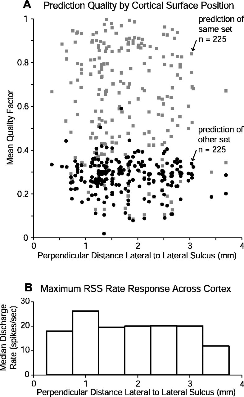
Population RSS prediction quality by electrode penetration position. A, Quality factors for same-set (gray rectangles) and other-set prediction (black circles) are shown for each unit of the population plotted against lateral distance, measured orthogonally from the lateral sulcus. No difference in prediction quality between A1 (less than ∼2 mm) and the lateral belt (more than ∼2 mm) becomes apparent, suggesting that linear analysis is not better suited for one of these cortical areas over the other. B, Median maximum RSS-induced discharge rate for the population shown in A is plotted against lateral distance, indicating that RSS can effectively drive stimuli in both cortical fields.

Relatively high sustained spiking rates were commonly found in these experiments. Some units spiked at rates of several hundred spikes per second, although the average was considerably lower. Figure 13B summarizes the RSS rates for units as a function of their lateral position. Plotted are the median discharge rates of the optimal RSS for each unit within the indicated 0.5 mm regions of cortex. Similarity in these rates across cortex indicates that RSS represent a reasonable stimulus choice for characterizing neurons in both A1 and the lateral belt.

Discussion

Responses of auditory cortical neurons to random spectrum stimuli

The fundamental assumption required to compute WFs for auditory cortical neurons is essentially satisfied in this experimental preparation: that the neuronal rate functions generate sustained discharge patterns of various rates for different stationary stimuli. Why, though, have sustained responses in auditory cortical neurons been so uncommonly seen in other preparations? Four separate factors probably contribute predominantly to this discrepancy.

First, most experimental preparations for studying auditory cortex have used anesthetized animals. Auditory cortex has long been known to be affected by anesthesia and to be affected differently by different kinds of anesthesia (Erulkar et al., 1956; Goldstein et al., 1959; Zurita et al., 1994; Kohn et al., 1996; Fitzpatrick et al., 2000; Cheung et al., 2001). Recent studies have found functional differences in the anesthetized and awake conditions in terms of phasic and tonic responses with more sustained firing patterns in the awake condition (Lu and Wang, 2000; Lu et al., 2001; Elhilali et al., 2002; Wang et al., 2002).

Second, if more than one population of neurons with different response properties is active in an awake preparation, then sampling bias caused by electrode tip geometry and impedance could conceivably skew the perceived proportion of phasic versus tonic neurons. At least one study of awake primate auditory cortex has reported that although large sustained responses could often be detected in the background signal of the extracellular electrode, only onset and weak sustained firing could be elicited from neurons isolated as single units (Brugge and Merzenich, 1973). We have observed a similar phenomenon in our own preparation when using low-impedance electrodes to study layer 4 neurons. Putative sample biases such as these may be ameliorated in part by electrode design.

Third, as has been shown in the examples of this paper, many neurons will generate sustained spiking patterns for near-optimal stationary stimuli, but suboptimal stimuli tend to generate either onset-only responses or suppressed spiking. The onset-only responses for these neurons are generally tuned, often mirroring the preferred frequency range of the sustained responses but with less selectivity. This tuning could lead to false interpretations of onset-only responses if stimulus sets of mostly suboptimal stimuli are used and the neurons are not probed extensively for their true stimulus preferences. Stimuli of extremely short duration represent one such potentially suboptimal stimulus set, especially for neurons with relatively long response latencies.

Fourth, stimulus optimality can involve more than simply placing stimulus energy in excitatory regions of a tuning function and eliminating energy from inhibitory regions. Neurons with complex stimulus preferences studied with suboptimal stimulus sets might never generate a spiking response to any stimulus tested (Barbour and Wang, 2003), thereby landing those neurons in the unresponsive discard bin. This loss of tonic yet selective neurons from further consideration could skew counts in favor of phasic responders.

Attempts to minimize errors contributing to overcounts of phasic responders in the current study can be summarized as follows. (1) These experiments were conducted in an awake primate; (2) high-impedance electrodes guaranteed high action potential waveform SNRs, and every neuron encountered in every cortical layer was tested and included in the final data set; (3) RSS were used to search a much wider portion of stimulus space than can be accessed using tones or bandpass noise alone; and (4) stimulus parameters were not explicitly predetermined but were varied on-line as necessary to match the preferences of the neurons.

Less than 10% of the significantly driven neurons generated onset-only responses to stationary stimuli (Fig. 4), even after extensive testing with many different RSS parameters. These neurons may respond in phasic manner if exposed to modulated RSS, in which case they would make excellent candidates for study with spectrotemporal receptive fields constructed from spike-triggered averages. It has been shown, however, that proper amplitude or frequency modulations of tones can evoke tonic responses from marmoset auditory cortex neurons that respond only at the onset of pure tones (Liang et al., 2002, their Fig. 17); therefore, onset-only neurons in response to RSS should be interpreted cautiously.

Linear spectral weighting function sensitivity to RSS parameters

Three main RSS parameters potentially capable of influencing WF shape were tested: mean level, spectral density, and spectral contrast. In all cases the results mirrored one another: these three parameters can change the magnitude of the WF but usually have little effect on the shape, especially near CF. WFs with larger magnitudes (higher estimate SNRs) generally resist shape alterations more than do those with smaller magnitudes.

For mean level, this invariance property tends to create “level-tolerant” RSS representations of frequency response. Level tolerance measured by pure tones has been interpreted in the literature to represent sharpening of frequency tuning by the process of lateral inhibition (Suga and Tsuzuki, 1985; Suga, 1995, 1997; Ehret and Schreiner, 1997; Sutter, 2000). The excitatory peaks of WFs seem to represent an invariant property of cortical neurons. This type of RSS level tolerance has been observed at other levels of the auditory system, including auditory nerve, cochlear nucleus, and inferior colliculus (Calhoun et al., 1998; Yu and Young, 2000, 2002), and therefore is not surprising in cortex. Its presence in both the auditory nerve and higher auditory stations, despite significant convergence of excitatory inputs, implies that cochlear properties and flanking inhibition may combine to preserve tuning to wideband sounds regardless of sound level.

Spectral density and spectral contrast variations share with shifts in mean level the potential to alter WFs because changes in these parameters induce changes in stimulus energy distribution across frequency. Changing density and contrast of the RSS, however, did not substantially alter the frequencies indicated by the WF to be excitatory or inhibitory, at least over the parameter ranges tested. The weight magnitudes often changed with contrast but rarely with density. As in the mean level case, WFs with larger magnitudes tended to be more resistant to shape alterations, probably because of estimate SNR effects.

To summarize the above findings, if an RSS set can elicit spikes from an auditory cortex neuron, then the resulting WF shape represents primarily stimulus-invariant tuning properties. This robustness does not necessarily imply that the neuron is linear throughout its dynamic range, just that the linear estimates of frequency tuning are relatively invariant over that dynamic range.

Predictive power of linear spectral weighting functions

Although uncorrelated stimuli formed from an orthonormal basis represent a convenient way to probe a large stimulus space efficiently, their greatest potential usefulness lies in the application of powerful reverse-correlation analytic methods to draw conclusions about stimulus-invariant neuronal properties (de Boer and Kuyper, 1968; de Boer and de Jongh, 1978; Johnson, 1980; Aertsen and Johannesma, 1981; Eggermont et al., 1983). Traditionally these methods have been used to assess how well a linear model of the response properties of a neuron accounts for the general behavior of the neuron, which intuitively must be nonlinear in nature. Particular input variables are not precluded from combining linearly, however, and claims have been made to that effect in auditory cortex (Kowalski et al., 1996; deCharms et al., 1998; Depireux et al., 2001; Schnupp et al., 2001).

The prediction data shown here reflect the easiest possible prediction task presentable to a linear model: given the observed responses to a stimulus set, predict the responses to a statistically identical, linearly related set of stimuli. The resulting quality factors for the entire data set shown in Figure 11 are uniformly low. Although quality factors for both the nearly linear chopper and decidedly nonlinear type IV cell types of the dorsal cochlear nucleus have been shown to have values this low at some sound levels (Yu and Young, 2000), the prediction task in that case was more difficult because the testing stimuli (wideband noise filtered by head-related transfer functions) represented a stimulus class unique from RSS. Furthermore, the highest quality factors for choppers were found in the center of their dynamic ranges, where weight values were greatest; this distribution mirrors that from which the cortical WFs were computed. The asymmetric cortical quality factors and subset of low same-set quality factors combine with the preceding results to indicate that auditory cortex neurons integrate frequency information nonlinearly. Perhaps because the onset responses are less stimulus selective than the sustained responses (Wang et al., 2002), studies eliciting only onset spikes may reveal a linear coding that is not seen under conditions favoring sustained spiking. In other words, perhaps suboptimal responses are primarily linear whereas the optimal responses are not.

The examples from Figure 10 reveal that much of the mismatch between WFs computed from paired RSS sets occurs away from CF. This result may not be surprising in hindsight, because intracellular studies have shown that auditory cortex neurons receive subthreshold excitatory and inhibitory projections from frequencies as far removed from CF as several octaves (de Ribaupierre et al., 1972, 1976; Serkov and Volkov, 1985; DeWeese and Zador, 2000) in a manner reminiscent of the “iceberg” effect in V1 (Creutzfeldt et al., 1974; Anderson et al., 2000; Carandini and Ferster, 2000). Asynchronous stimulation at these frequencies apparently can push some of these responses above threshold, revealing a stimulus-dependent spectrotemporal receptive field (Blake and Merzenich, 2002). Lateral belt neurons were also driven by RSS but exhibited neither better nor worse predictions than did A1 neurons (Fig. 13). When used for prediction, WFs apparently do not reveal unique classes of neurons distributed throughout auditory cortex.

Finally, although linear spectral weighting functions may not reveal significant linearity in auditory cortex, their ability to elicit sustained discharges from most cortical neurons and their robustness in the face of random spectrum stimulus parameter variation makes them a potentially useful tool for exploring fundamental characteristics of these neurons.

References

- Abeles M, Goldstein Jr MH ( 1970) Functional architecture in cat primary auditory cortex: columnar organization and organization according to depth. J Neurophysiol 33: 172-187. [DOI] [PubMed] [Google Scholar]
- Abeles M, Goldstein Jr MH ( 1972) Responses of single units in the primary auditory cortex of the cat to tones and to tone pairs. Brain Res 42: 337-352. [DOI] [PubMed] [Google Scholar]
- Aertsen AM, Johannesma PI ( 1981) The spectro-temporal receptive field. A functional characteristic of auditory neurons. Biol Cybern 42: 133-143. [DOI] [PubMed] [Google Scholar]
- Anderson JS, Lampl I, Gillespie DC, Ferster D ( 2000) The contribution of noise to contrast invariance of orientation tuning in cat visual cortex. Science 290: 1968-1972. [DOI] [PubMed] [Google Scholar]
- Barbour DL, Wang X ( 2002) Temporal coherence sensitivity in auditory cortex. J Neurophysiol 88: 2684-2699. [DOI] [PubMed] [Google Scholar]
- Barbour DL, Wang X ( 2003) Contrast tuning in auditory cortex. Science 299: 1073-1075. [DOI] [PMC free article] [PubMed] [Google Scholar]
- Blake DT, Merzenich MM ( 2002) Changes of AI receptive fields with sound density. J Neurophysiol 88: 3409-3420. [DOI] [PubMed] [Google Scholar]
- Brugge JF, Merzenich MM ( 1973) Responses of neurons in auditory cortex of the macaque monkey to monaural and binaural stimulation. J Neurophysiol 36: 1138-1158. [DOI] [PubMed] [Google Scholar]
- Brugge JF, Dubrovsky NA, Aitkin LM, Anderson DJ ( 1969) Sensitivity of single neurons in auditory cortex of cat to binaural tonal stimulation: effects of varying interaural time and intensity. J Neurophysiol 32: 1005-1024. [DOI] [PubMed] [Google Scholar]
- Calhoun BM, Miller RL, Wong JC, Young ED ( 1998) Rate encoding of stimulus spectra by auditory nerve fibers. In: Psychophysical and physiological advances in hearing (Palmer AR, Rees A, Summerfield AQ, Meddis R, eds), pp 170-177.
- London: Whurr. Carandini M, Ferster D ( 2000) Membrane potential and firing rate in cat primary visual cortex. J Neurosci 20: 470-484. [DOI] [PMC free article] [PubMed] [Google Scholar]
- Cheung SW, Nagarajan SS, Bedenbaugh PH, Schreiner CE, Wang X, Wong A ( 2001) Auditory cortical neuron response differences under isoflurane versus pentobarbital anesthesia. Hear Res 156: 115-127. [DOI] [PubMed] [Google Scholar]
- Creutzfeldt O, Innocenti GM, Brooks D ( 1974) Vertical organization in the visual cortex (area 17) in the cat. Exp Brain Res 21: 315-336. [DOI] [PubMed] [Google Scholar]
- de Boer E, de Jongh HR ( 1978) On cochlear encoding: potentialities and limitations of the reverse-correlation technique. J Acoust Soc Am 63: 115-135. [DOI] [PubMed] [Google Scholar]
- de Boer E, Kuyper P ( 1968) Triggered correlation. IEEE Trans Biomed Eng 15: 169-179. [DOI] [PubMed] [Google Scholar]
- deCharms RC, Blake DT, Merzenich MM ( 1998) Optimizing sound features for cortical neurons. Science 280: 1439-1443. [DOI] [PubMed] [Google Scholar]
- Depireux DA, Simon JZ, Klein DJ, Shamma SA ( 2001) Spectro-temporal response field characterization with dynamic ripples in ferret primary auditory cortex. J Neurophysiol 85: 1220-1234. [DOI] [PubMed] [Google Scholar]
- de Ribaupierre F ( 1976) Coding of the acoustic information in the superior auditory centers. Bull Schweiz Akad Med Wiss 32: 29-39. [PubMed] [Google Scholar]
- de Ribaupierre F, Goldstein MH, Yeni-Komshian G ( 1972) Intracellular study of the cat's primary auditory cortex. Brain Res 48: 185-204. [DOI] [PubMed] [Google Scholar]
- DeWeese MR, Zador A ( 2000) In vivo whole cell recordings of synaptic responses to acoustic stimuli in rat auditory cortex. Soc Neurosci Abstr 26: 1704. [Google Scholar]
- Efron B, Tibshirani RJ ( 1993) An introduction to the bootstrap. New York: Chapman and Hall.
- Eggermont JJ ( 1997) Firing rate and firing synchrony distinguish dynamic from steady state sound. NeuroReport 8: 2709-2713. [DOI] [PubMed] [Google Scholar]
- Eggermont JJ, Johannesma PM, Aertsen AM ( 1983) Reverse-correlation methods in auditory research. Q Rev Biophys 16: 341-414. [DOI] [PubMed] [Google Scholar]
- Ehret G, Schreiner CE ( 1997) Frequency resolution and spectral integration (critical band analysis) in single units of the cat primary auditory cortex. J Comp Physiol [A] 181: 635-650. [DOI] [PubMed] [Google Scholar]
- Elhilali M, Fritz JB, Bozak D, Depireux DA, Shamma SA ( 2002) Comparison of response characteristics in auditory cortex of the awake and anesthetized ferret. Assoc Res Otolaryngol Abstr 25: 42. [Google Scholar]
- Erulkar SD, Rose JE, Davies PW ( 1956) Single unit activity in the auditory cortex of the cat. Bull Johns Hopkins Hosp 99: 55-86. [PubMed] [Google Scholar]
- Evans EF, Ross HF, Whitfield IC ( 1965) The spatial distribution of unit characteristic frequency in the primary auditory cortex of the cat. J Physiol (Lond) 179: 238-247. [DOI] [PMC free article] [PubMed] [Google Scholar]
- Fitzpatrick DC, Kuwada S, Batra R ( 2000) Neural sensitivity to interaural time differences: beyond the Jeffress model. J Neurosci 20: 1605-1615. [DOI] [PMC free article] [PubMed] [Google Scholar]
- Furukawa S, Xu L, Middlebrooks JC ( 2000) Coding of sound-source location by ensembles of cortical neurons. J Neurosci 20: 1216-1228. [DOI] [PMC free article] [PubMed] [Google Scholar]
- Goldstein MH, Abeles M ( 1975a) Single unit activity of the auditory cortex. In: Handbook of sensory physiology (Keidel WD, Neff WD, eds), pp 199-218.
- Berlin: Springer. Goldstein Jr MH, Abeles M ( 1975b) Note on tonotopic organization of primary auditory cortex in the cat. Brain Res 100: 188-191. [DOI] [PubMed] [Google Scholar]
- Goldstein MH, Kiang NY, Brown RM ( 1959) Response of the auditory cortex to repetitive acoustic stimuli. J Acoust Soc Am 31: 356-364. [Google Scholar]
- Goldstein Jr MH, Abeles M, Daly RL, McIntosh J ( 1970) Functional architecture in cat primary auditory cortex: tonotopic organization. J Neurophysiol 33: 188-197. [DOI] [PubMed] [Google Scholar]
- Heil P ( 1997a) Auditory cortical onset responses revisited. I. First-spike timing. J Neurophysiol 77: 2616-2641. [DOI] [PubMed] [Google Scholar]
- Heil P ( 1997b) Auditory cortical onset responses revisited. II. Response strength. J Neurophysiol 77: 2642-2660. [DOI] [PubMed] [Google Scholar]
- Johnson DH ( 1980) Applicability of white-noise nonlinear system analysis to the peripheral auditory system. J Acoust Soc Am 68: 876-884. [DOI] [PubMed] [Google Scholar]
- Klein DJ, Depireux DA, Simon JZ, Shamma SA ( 2000) Robust spectrotemporal reverse correlation for the auditory system: optimizing stimulus design. J Comput Neurosci 9: 85-111. [DOI] [PubMed] [Google Scholar]
- Kohn AZ, Depireux DA, Shamma SA ( 1996) Effects of different anesthetics on the responses to broadband sounds in the ferret primary auditory cortex and inferior colliculus. Soc Neurosci Abstr 22: 1067. [Google Scholar]
- Kowalski N, Depireux DA, Shamma SA ( 1996) Analysis of dynamic spectra in ferret primary auditory cortex. II. Prediction of unit responses to arbitrary dynamic spectra. J Neurophysiol 76: 3524-3534. [DOI] [PubMed] [Google Scholar]
- Liang L, Lu T, Wang X ( 2002) Neural representations of sinusoidal amplitude and frequency modulations in the primary auditory cortex of awake primates. J Neurophysiol 87: 2237-2261. [DOI] [PubMed] [Google Scholar]
- Lu T, Wang X ( 2000) Temporal discharge patterns evoked by rapid sequences of wide- and narrowband clicks in the primary auditory cortex of cat. J Neurophysiol 84: 236-246. [DOI] [PubMed] [Google Scholar]
- Lu T, Liang L, Wang X ( 2001) Temporal and rate representations of time-varying signals in the auditory cortex of awake primates. Nat Neurosci 4: 1131-1138. [DOI] [PubMed] [Google Scholar]
- Luenberger DG ( 1969) Optimization by vector space methods. New York: Wiley.
- Merzenich MM, Knight PL, Roth GL ( 1973) Cochleotopic organization of primary auditory cortex in the cat. Brain Res 63: 343-346. [DOI] [PubMed] [Google Scholar]
- Merzenich MM, Knight PL, Roth GL ( 1975) Representation of cochlea within primary auditory cortex in the cat. J Neurophysiol 38: 231-249. [DOI] [PubMed] [Google Scholar]
- Miller JM, Dobie RA, Pfingst BE, Hienz RD ( 1980) Electrophysiologic studies of the auditory cortex in the awake monkey. Am J Otolaryngol 1: 119-130. [DOI] [PubMed] [Google Scholar]
- Miller LM, Escabi MA, Read HL, Schreiner CE ( 2002) Spectrotemporal receptive fields in the lemniscal auditory thalamus and cortex. J Neurophysiol 87: 516-527. [DOI] [PubMed] [Google Scholar]
- Phillips DP ( 1988) Effect of tone-pulse rise time on rate-level functions of cat auditory cortex neurons: excitatory and inhibitory processes shaping responses to tone onset. J Neurophysiol 59: 1524-1539. [DOI] [PubMed] [Google Scholar]
- Phillips DP, Sark SA ( 1991) Separate mechanisms control spike numbers and inter-spike intervals in transient responses of cat auditory cortex neurons. Hear Res 53: 17-27. [DOI] [PubMed] [Google Scholar]
- Phillips DP, Kitzes LM, Semple MN, Hall SE ( 1996) Stimulus-induced spike bursts in two fields of cat auditory cortex. Hear Res 97: 165-173. [PubMed] [Google Scholar]
- Poldrack RA, Temple E, Protopapas A, Nagarajan S, Tallal P, Merzenich M, Gabrieli JD ( 2001) Relations between the neural bases of dynamic auditory processing and phonological processing: evidence from fMRI. J Cognit Neurosci 13: 687-697. [DOI] [PubMed] [Google Scholar]
- Rauschecker JP ( 1997) Processing of complex sounds in the auditory cortex of cat, monkey, and man. Acta Otolaryngol [Suppl] 532: 34-38. [DOI] [PubMed] [Google Scholar]
- Rauschecker JP, Tian B, Hauser M ( 1995) Processing of complex sounds in the macaque nonprimary auditory cortex. Science 268: 111-114. [DOI] [PubMed] [Google Scholar]
- Recanzone GH ( 2000) Response profiles of auditory cortical neurons to tones and noise in behaving macaque monkeys. Hear Res 150: 104-118. [DOI] [PubMed] [Google Scholar]
- Schnupp JW, Mrsic-Flogel TD, King AJ ( 2001) Linear processing of spatial cues in primary auditory cortex. Nature 414: 200-204. [DOI] [PubMed] [Google Scholar]
- Schreiner CE, Calhoun BM ( 1994) Spectral envelope coding in cat primary auditory cortex: properties of ripple transfer functions. Audit Neurosci 1: 39-61. [Google Scholar]
- Schreiner CE, Urbas JV ( 1986) Representation of amplitude modulation in the auditory cortex of the cat. I. The anterior auditory field (AAF). Hear Res 21: 227-241. [DOI] [PubMed] [Google Scholar]
- Serkov FN, Volkov IO ( 1985) Role of cortical inhibition in the analysis of auditory stimuli. Fiziol Zh 31: 569-578. [PubMed] [Google Scholar]
- Shamma SA, Fleshman JW, Wiser PR, Versnel H ( 1993) Organization of response areas in ferret primary auditory cortex. J Neurophysiol 69: 367-383. [DOI] [PubMed] [Google Scholar]
- Shamma SA, Versnel H, Kowalski N ( 1995) Ripple analysis in ferret primary auditory cortex. I. Response characteristics of single units to sinusoidally rippled spectra. Audit Neurosci 1: 233-254. [Google Scholar]
- Suga N ( 1995) Sharpening of frequency tuning by inhibition in the central auditory system: tribute to Yasuji Katsuki. Neurosci Res 21: 287-299. [DOI] [PubMed] [Google Scholar]
- Suga N ( 1997) Tribute to Yasuji Katsuki's major findings: sharpening of frequency tuning in the central auditory system. Acta Otolaryngol [Suppl] 532: 9-12. [DOI] [PubMed] [Google Scholar]
- Suga N, Tsuzuki K ( 1985) Inhibition and level-tolerant frequency tuning in the auditory cortex of the mustached bat. J Neurophysiol 53: 1109-1145. [DOI] [PubMed] [Google Scholar]
- Sutter ML ( 2000) Shapes and level tolerances of frequency tuning curves inprimary auditory cortex: quantitative measures and population codes. J Neurophysiol 84: 1012-1025. [DOI] [PubMed] [Google Scholar]
- Theunissen FE, Sen K, Doupe AJ ( 2000) Spectral-temporal receptive fields of nonlinear auditory neurons obtained using natural sounds. J Neurosci 20: 2315-2331. [DOI] [PMC free article] [PubMed] [Google Scholar]
- Versnel H, Shamma SA ( 1998) Spectral-ripple representation of steady-state vowels in primary auditory cortex. J Acoust Soc Am 103: 2502-2514. [DOI] [PubMed] [Google Scholar]
- Wang X, Lu T, Liang L ( 2002) Emergence of sustained discharges in auditory cortex under awake conditions. Assoc Res Otolaryngol Abstr 25: 119. [Google Scholar]
- Wang X, Merzenich MM, Beitel R, Schreiner CE ( 1995) Representation of a species-specific vocalization in the primary auditory cortex of the common marmoset: temporal and spectral characteristics. J Neurophysiol 74: 2685-2706. [DOI] [PubMed] [Google Scholar]
- Woolsey CN, Walzl EM ( 1942) Topical projections of nerve fibers from local regions of the cochlea to the cerebral cortex of the cat. Bull Johns Hopkins Hosp 71: 315-344. [Google Scholar]
- Yu JJ, Young ED ( 2000) Linear and nonlinear pathways of spectral information transmission in the cochlear nucleus. Proc Natl Acad Sci USA 97: 11780-11786. [DOI] [PMC free article] [PubMed] [Google Scholar]
- Yu JJ, Young ED ( 2002) Segregation of spectral information processing among neural populations in the inferior colliculus. Assoc Res Otolaryngol Abstr 25: 39. [Google Scholar]
- Zurita P, Villa AE, de Ribaupierre Y, de Ribaupierre F, Rouiller EM ( 1994) Changes of single unit activity in the cat's auditory thalamus and cortex associated to different anesthetic conditions. Neurosci Res 19: 303-316. [DOI] [PubMed] [Google Scholar]