New methods for inferring population dynamics from microbial sequences

Abstract

The reduced cost of high throughput sequencing, increasing automation, and the amenability of sequence data for evolutionary analysis are making DNA data (or the corresponding amino acid sequences) the molecular marker of choice for studying microbial population genetics and phylogenetics. Concomitantly, due to the ever-increasing computational power, new, more accurate (and sometimes faster), sequence-based analytical approaches are being developed and applied to these new data. Here we review some commonly used, recently improved, and newly developed methodologies for inferring population dynamics and evolutionary relationships using nucleotide and amino acid sequence data, including: alignment, model selection, bifurcating and network phylogenetic approaches, and methods for estimating demographic history, population structure, and population parameters (recombination, genetic diversity, growth, and natural selection). Because of the extensive literature published on these topics this review cannot be comprehensive in its scope. Instead, for all the methods discussed we introduce the approaches we think are particularly useful for analyses of microbial sequences and where possible, include references to recent and more inclusive reviews.

1. Introduction

Although nucleotide and amino acid sequence-based approaches have been used in the past for inferring microbial evolutionary relationships, in the last few years these methods have been increasingly used for typing and characterizing their populations (Maiden et al., 1998; Crandall, 1999; Urwin and Maiden, 2003; Cooper and Feil, 2004). Sequencing methods provide standardized and unambiguous data that are portable through web-based databases with direct access to the information needed to identify and monitor emerging pathogenic agents (Chan et al., 2001; Feil et al., 2004; Spratt et al., 2004). More importantly, sequence data, unlike many other forms of molecular typing data, provide direct genealogical information that can be used efficiently to estimate phylogenetic relationships and parameters associated with population dynamics. Therefore, the application of appropriate analytical tools makes it possible to extract the maximum population genetic and evolutionary inference from the data produced. These inferences can, in turn, be used to improve public health control strategies (Wiedmann, 2002).

This review presents analytical methods used for inferring population dynamics and phylogenies using DNA and amino acid sequences (Fig. 1). However, because of the large number of analytical tools treated here this study cannot be comprehensive in its scope. Some methods, such as those for the detection and estimation of recombination, have been thoroughly reviewed in recent papers, so the reader is referred to those studies; other methods, however, such as those for the estimation of adaptive selection, have not, so they are considered here in more detail. A list and description of what we think are the most appropriate approaches for the analysis of microbial sequences is provided for all the analytical sections addressed here. The decision for choosing a particular method over any other is based on its adequacy for analyzing microbial sequence data, performance assessment (published studies and personal experience), and software implementation. The assumptions made by the various approaches proposed are also different and some times mutually exclusive. So the user must choose carefully the methods for data analyses and the associated research goals. Moreover, the evolutionary analysis of sequence data is a rapidly advancing field, with continual improvement of existing methodologies and algorithms. Hence, our hope here is that this review will provide a useful starting point and guide to methods of sequence analysis suitable for microbial phylogenetics and population inference.

Fig. 1.

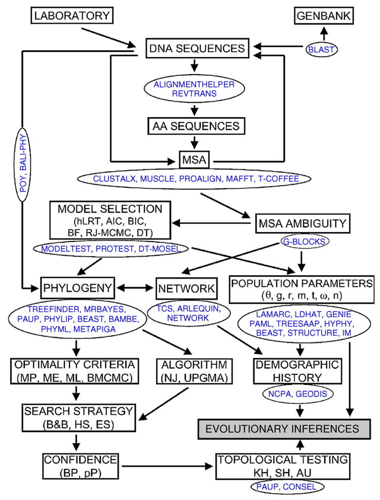
Flow chart showing the application of various analytical approaches applied to molecular data for inferring microbial population dynamics. Abbreviations are explained in the main text.

2. Alignment strategies

Any phylogenetic or population study of sequence data usually begins with a multiple sequence alignment (MSA) of homologous molecules. Since “alignment strategies” are the first point of our review, we will simply assume that the sequences of interest descended from a common ancestor; however, sequence homology must always be assessed before and after estimating an alignment. A MSA is an hypothesis of homology for each nucleotide or amino acid (AA) position in the data. For closely related taxa (e.g., clones from the same strain), highly conserved gene regions (e.g., stems in ribosomal genes), or protein coding genes (e.g., housekeeping genes), the estimation of a MSA can be trivial and established by visual inspection. But at deeper phylogenetic levels or when working with fast-evolving genes (e.g., the envelope gene in HIV), alignment can be far from trivial and insertion and deletion events (indels or gaps) must be postulated. Inferring a MSA of AAs is computationally easier than the alignment of nucleotides because the AA alphabet is composed of 20 characters while DNA only has 4. Thus, the “signal-to-noise ratio” is much better in AA than nucleotide sequences (not to mention there are two-thirds fewer characters to align for AAs for a given sequence). Therefore, when analyzing protein-coding genes, the problem of inferring positional homology can be simplified by first translating the DNA sequences into AAs, aligning the resulting peptide sequences, and then converting them back to nucleotides.

Computer programs such as ALIGNMENTHELPER (http://www.inbio.byu.edu/faculty/dam83/cdm) and REVTRANS (Wernersson and Pedersen, 2003) can perform this task. Even if the alignment is straightforward, coding sequences must always be aligned using a sequence editor that is capable of toggling between AA and nucleotides to be sure that the appropriate reading frame is maintained; otherwise, errors can jeopardize subsequent analyses (e.g., tests of adaptive selection). Popular sequence editors are MACCLADE (Maddison and Maddison, 2000), SE-AL (http://www.evolve.zoo.ox.ac.uk/software.html), BIOEDIT (http://www.mbio.ncsu.edu/Bioedit/bioedit.html), and SQUINT (http://www.bioinformatics.org.nz/).

2.1. What MSA method to choose?

This is a difficult question, given the variety of methods for assembling a MSA. In fact, all of the available methods use approximations (heuristics). Moreover, observed performance differences in comparative analyses (see below) usually emerge as average estimates; hence approaches that work well for a certain gene or protein family may not work as well for a different one. Therefore, as a standard procedure, one should use multiple alignment approaches and parameter sets and carefully inspect the results (see reviews by Duret and Abdeddaim, 2000; Notredame, 2002). Here we will review different global alignment procedures (i.e., the sequences are related over their whole length) to perform MSA. Alignment is one of the most important but ironically underappreciated and neglected aspects of sequence analysis (Felsenstein, 2004; Crandall et al., 2005); hence we will endeavor to explain the strategies underlying some of the most commonly used algorithms, as well as their strengths and caveats.

2.1.1. Progressive algorithms

Progressive alignment algorithms are by far the most widely used because of their speed, simplicity, and efficiency. The basic strategy of these methods is first to estimate a tree and then to construct a pairwise alignment of the subtrees found at each internal node. More sophisticated algorithms (e.g., iterative algorithms) also use this basic strategy in the initial or final steps of their routines. The most frequently used progressive algorithm is that implemented in CLUSTALW (Thompson et al., 1994) and its window interface CLUSTALX (Thompson et al., 1997). The basic MSA algorithm consists of three main stages: (i) all pairs of sequences are aligned separately and an uncorrected distance matrix is calculated; (ii) a guide tree (neighbor-joining tree, Saitou and Nei, 1987) is calculated from the distance matrix; (iii) the sequences are progressively aligned (profile alignment) according to the branching order in the guide tree. The main caveat of this strategy is that any misaligned regions created early in the process cannot be corrected later as new sequences are added. Benchmarking tests (i.e., databases of reference structural alignments used to assess performance of MSA methods) carried out in BALiBASE (Thompson et al., 1999a) showed that CLUSTALW performs better when the phylogenetic tree is relatively dense without any obvious outliers (Thompson et al., 1999b). Long insertions or deletions can also be problematic due to the intrinsic limitation of the implemented affine penalty scheme. CLUSTALX includes quality analysis tools, which allow for the identification of problematic regions and realigning by adjusting the gap penalties (i.e., refinement). The application TuneCLUSTALX (http://www.homepage.mac.com/barryghall/Software.html) run in conjunction with CLUSTALX can aid in constructing a better alignment. CLUSTAL can align both nucleotides and AAs. For the latter, BLOSUM, PAM, GONNET, and identity matrixes can be implemented. It can also use SwissProt secondary structure information.

2.1.2. Consistency-based algorithms

An improved progressive strategy is implemented in T-COFFEE (Notredame et al., 2000) where sequences are aligned in a progressive manner but using a consistency-based objective function that minimizes potential errors in the early stages of the alignment assembly. It works as follows: first it generates two primary libraries of pairwise global CLUSTALW and local LALIGN (PASTA package, Pearson and Lipman, 1988) alignments and assigns weights to each pair; then both libraries are combined in a new primary library by a process of addition and weights are re-estimated; a position-specific substitution matrix (extended library) is then created by examining the consistency of each pair of residues with residue pairs from all of the other alignments; this new library (and weights) is finally resolved by using a progressive alignment strategy similar to that implemented in CLUSTAL to give a MSA. Comparison with CLUSTALW using the BALiBASE database indicates that T-COFFEE is significantly more accurate, but about two times slower. A novel method (3DCOFFEE) has been published (O’Sullivan et al., 2004) that combines protein sequences and SD-structures in order to generate high-quality MSA.

2.1.3. Iterative algorithms

The strategy here is to produce an alignment using the progressive approach and then refine it through a series of cycles (iterations) until no more improvements can be made. Examples of methods implementing this strategy are MUSCLE (Edgar, 2004) and MAFFT (Katoh et al., 2002, 2005), the fastest known algorithms. MUSCLE generates a refined alignment in three basic steps. In an initial stage (draft progressive), it produces a MSA 1 quickly (speed is emphasized over accuracy) using uncorrected distances and the UPGMA (TREE1) method. In a second stage (improved progressive), an improved MSA2 is generated by re-estimating a new guide tree (TREE2) using the Kimura two-parameter distance, which corrects for multiple substitutions per site. In a final stage (refinement) TREE2 is divided into two subtrees for which two profiles are computed. A new MSA is then produced by realigning the two profiles (MSA3). If MSA3 has a better score than MSA2 (as indicated by the log-expectation function implemented), then the new alignment is kept; otherwise, it is discarded. The refinement ends when convergence is reached. MUSCLE implements three different protein profile scoring functions: log-expectation score (it gives the best results and is also the only option for nucleotides), and sum of pairs score using either the PAM200 matrix or the VTML240 matrix. MAFFT (Katoh et al., 2005) implements a similar strategy, but offers a multiple array of algorithms for the progressive and refinement processes that implement a Fourier transform approximation and include local or global pairwise alignment information. Moreover, the user can choose among different AA scoring matrixes: BLOSUM (the most accurate), PAM, and JTT.

Notredame et al. (2000), Edgar (2004), and Katoh et al. (2005) compared the performance of these four programs using multiple benchmark alignment databases. The results can be summarized as follows for speed: MUSCLE > MAFFT > CLUSTALW > T-COFFEE; and accuracy: MAFFT > MUSCLE > T-COFFEE > CLUSTALW. However, these relative comparisons must be interpreted with caution because the results are averaged over large numbers of tests and did not include the same (or most recent) versions of the tested software.

2.1.4. Hidden Markov methods (HMM)-based algorithms

HMMs describe the MSA in a statistical context, using a Bayesian approach (see phylogenetic inference). From a formal point of view they are very attractive because they assign pP (posterior probability) values to particular MSA and sites, which allows a statistical evaluation of alternative alignments and identification of unreliable alignment regions, but it has the burden of being computationally intense (i.e., limited to small data sets of ~25 taxa). PROALIGN (Löytynoja and Milinkovitch, 2003) is an example of this approach that combines a pair of HMMs, a progressive algorithm, and an evolutionary model (see Section 3) describing the nucleotide or AA substitution process and the occurrence of gaps. This combination allegedly improves the accuracy of MSA and our understanding of the history and function of the sequences. Comparative performance tests with CLUSTALW using simulated data and the BALiBASE database indicated that PROALIGN was more accurate, albeit slower, for the aligning of nucleotide data.

2.2. Treating highly divergent segments of the alignment

Since not all gene regions evolve at the same rate (e.g., stem versus loop regions of ribosomal RNA), some parts of the MSA are reasonably conserved whereas others are very divergent and full of gaps, hence positional homology cannot always be precisely determined. In such cases, some authors (e.g., Gatesy et al., 1993; Swofford et al., 1996) recommend deleting those regions from subsequent analyses because they can be misleading. This is usually done in an arbitrary way, which makes the final alignment irreproducible. Some of the methods described above (e.g., CLUSTALX) can help to identify those poorly aligned regions, but more objective approaches such as GBLOCKS (Castresana, 2000) have been described for removing very divergent regions or gap positions from an alignment of DNA or protein sequences. GBLOCKS selects ambiguous blocks from the MSA according to a simple set of alignment positions features, including minimum number of sequences for a conserved and a flank position, maximum number of contiguous non-conserved positions, minimum length of a block, and allowed gap positions.

3. Model selection: beyond K2P

Model specification is a critical issue in molecular phylogenetics and population inference, as the implemented model (or lack thereof) affects most downstream analyses, including estimates of phylogeny, substitution rates, bootstrap values, posterior probabilities, tests of the molecular clock (Tamura, 1994; Yang et al., 1995; Sullivan and Swofford, 1997, 2001; Kelsey et al., 1999; Zhang, 1999; Buckley et al., 2001; Buckley, 2002; Buckley and Cunningham, 2002; Pupko et al., 2002; Suzuki et al., 2002) and estimates of key population parameters such as genetic diversity, recombination, growth, and natural selection (Yang et al., 2000; McVean et al., 2002; Posada et al., 2002; Kuhner et al., 2005). The issue of using the best-fit model is made even more crucial as new phylogenetic and coalescent methods (see population inference) are increasingly dependent on explicitly model-based methods requiring that the chosen model be justified and tuned to the data. In fact, the ability to select models within a rigorous statistical framework is one of the many advantages of explicitly model-based methods. Yet many researchers using these methods still rely on program defined default parameter values and models (e.g., JC, K2P), even though numerous studies have shown that phylogenetic methods are less accurate or become inconsistent when the model of evolution is misspecified (Felsenstein, 1978; Huelsenbeck and Hillis, 1993; Penny et al., 1994; Gaut and Lewis, 1995; Sullivan and Swofford, 1997; Bruno and Halpern, 1999; Yang and Bielawski, 2000). Regardless of data type (i.e., nucleotide or amino acid sequences), identifying the most appropriate model is essential to increasing the accuracy, consistency, and confidence of phylogenetic analyses and population parameter estimation. Therefore, how do we choose the best-fit model for our sequence data? This issue is usually assessed within a phylogenetic framework and has received a great deal of attention recently, leading to a suite of new methodologies (see Posada and Buckley, 2004; Sullivan and Joyce, 2005). In this section, we briefly review the available methods of model selection for both nucleotide and amino acid data, so that researchers studying microbial evolution can move beyond the ‘K2P perspective’.

3.1. Nucleotide data

Although model choice is a crucial part of phylogeny estimation, selecting a set from the 203 ‘standard’ time-reversible models of nucleotide substitution is not easy, especially when most model selection methods are limited to a subset of these (Huelsenbeck et al., 2004; Posada and Buckley, 2004). Model choice will be complicated further by increasing complexity, as parameters reflecting new information on nucleotide substitution processes are added to candidate models. Furthermore, model selection is moving towards using confidence sets of models for phylogeny estimation by estimating a tree for each candidate model in a 95% confidence set and then building a consensus tree using model weights (Akaike weights, BIC weights, or model likelihoods from Bayesian analyses) as tree weights (Posada and Buckley, 2004). Although a crucial step in phylogeny estimation, there is ‘no substitute for careful thinking and common sense reasoning’ when selecting the model of evolution (Browne, 2000).

3.1.1. hLRTs

In 1997, Huelsenbeck and Crandall (1997), Frati et al. (1997) and Sullivan et al. (1997), all proposed a method of model selection involving successive pairwise comparisons of nested models using hierarchical likelihood ratio tests (hLRTs) to determine the best-fit model at each step. These pairwise comparisons are made in a specific sequence until a model is found that cannot be rejected. This suggested methodology was later implemented in the program MODELTEST (Posada and Crandall, 1998), which works in conjunction with the commonly used phylogenetic analysis program PAUP* (Swofford, 2002) to test 56 models of evolution. Since then, hLRTs have become the most widely used strategy of model selection. However, while hLRTs are a huge improvement over arbitrary model choice (or no choice at all), recent studies have shown that hLRTs have some undesirable characteristics. First, hLRT methods attempt to find the model that best fits the data under the assumption that at least one of the models compared is correct, even though all candidate models will be misspecified (i.e., the ‘true model’ is unknown). Furthermore, hLRTs perform multiple tests with the same data, which will increase the rate of false positives, and the model chosen can be affected by whether the pairwise comparisons start with either the simplest or most complex models. hLRT methods are also unable to accomplish model averaging or assess model selection uncertainty. Finally, hLRTs can only provide information regarding the relative fit of the nested alternatives, but cannot evaluate the absolute goodness of fit of the chosen model (Minin et al., 2003).

3.1.2. AIC

To overcome some of the issues surrounding the use of hLRTs, more recent model selection methods (MOLPHY, Adachi and Hasegawa, 1996; Modeltest, Posada and Crandall, 1998) implement several estimators (AIC differences, Akaike weights) based on the Akaike Information Criterion (AIC) for evaluating model fit (Posada and Buckley, 2004). In a phylogenetic context, AIC is designed to choose the model that best approximates reality and represents the amount of information lost when using a given model to approximate the real process of nucleotide substitution (Posada and Buckley, 2004). In comparison to hLRTs, AIC statistics have the advantage of being able to simultaneously compare all candidate models (nested and non-nested), assess model selection uncertainty, and allow for model-averaged parameter estimates and relative parameter importance. Furthermore, whereas hLRTs tend to favor more complex models (Burnham and Anderson, 2002), AIC includes a penalty for over-parameterization (Sullivan and Joyce, 2005). In addition to the original AIC, there are several derived AIC statistics used for model selection: the second order AIC, AIC_c, should be used when sample size (n) is small compared to the number of parameters (K); because AIC is a relative score, AIC differences can be used to rank candidate models, with larger AIC differences being less probable; Akaike weights (w) can be used for assessing model selection uncertainty by constructing 95% confidence sets of models by summing w from largest to smallest.

3.1.3. Bayesian methods

Although Bayesian methods as applied to both phylogenetic and population parameter inference are relatively new, either model selection and/or the estimation of the model parameters in an a priori specified model can be an integral part of these analyses. Bayesian approaches of model selection are designed to identify the true model given the data and they have several advantages over standard hLRTs, including the ability to compare non-nested sets of models and to make inferences based on the entire set of candidate models (i.e., model averaging). Additionally, Bayesian model selection methods are not dependent on a single topology or a particular set of model parameters, making the results more valid (Nylander et al., 2004). Model selection can be incorporated into this framework in several ways, including the use of pP, Bayesian information criterion (BIC), and Bayes factors (BF). Perhaps the most common way of assessing confidence in a hypothesis (or model of evolution) within a Bayesian framework is to choose the solution with the highest pP; furthermore, model uncertainty can be accounted for by ranking models according to their pP and constructing a 95% credible interval by summing these probabilities. However, calculating model pP can be computationally intensive. The BIC offers a more computationally feasible approach than calculating model likelihoods (Schwarz, 1978). BIC statistics also allow for simultaneous comparison of multiple models.

The third method of model selection in Bayesian analyses is the use of BF. Similar to hLRT methods, BF consist of multiple pairwise comparisons of evidence provided by the data for two competing models (Kass and Raftery, 1995; Raftery, 1996) and is already being used for model selection in phylogenetics (Suchard et al., 2001; Aris-Brosou and Yang, 2002; Huelsenbeck et al., 2004; Nylander et al., 2004). Although the interpretation of BF are up to the investigator, the general guidelines state that BF scores >150 are very strong evidence for a model, 20–50 is strong, 3–20 is positive, 1–3 barely worth mentioning, and if <1 there is evidence for the competing model (Kass and Raftery, 1995; Raftery, 1996). However, because BF consist of pairwise comparisons, this statistic may have some of the same issues as hLRTs. While studies with empirical data have shown BF to be useful for selecting among complex models, it is still unclear whether this statistic represents a reasonable balance between model complexity and error in parameter estimates (Nylander et al., 2004).

Another advantage of Bayesian methodology is the ability to directly obtain a model-averaged estimate of phylogeny using an algorithm that moves through both parameter and model space (Green, 1995). This type of ‘reversible jump Markov chain Monte Carlo’ algorithm (RJ-MCMC) has recently been implemented by Huelsenbeck et al. (2004). RJ-MCMC combines model selection and phylogeny into a single step, allowing for the screening of a large number of complex candidate models while performing a phylogenetic analysis. In contrast to other model selection statistics that are limited to a small set of candidate models, this method is capable of evaluating all possible time-reversible models while accounting for uncertainty in the model during phylogeny estimation. RJ-MCMC accomplishes this feat by implementing a MCMC algorithm that jumps between models visiting each in proportion to the posterior distribution, allowing calculation of BF for any of the models and for averaging over the possible models while performing phylogeny estimation (Huelsenbeck et al., 2004).

Even with these differences, the Bayesian and likelihood approaches seem to arrive at similar results (Nylander et al., 2004). In comparative studies of model selection, Huelsenbeck et al. (2004) found that AIC, BIC, posterior probabilities, BF, and RJ-MCMC are largely concordant, either choosing the same ‘best’ model or choosing a model within the 95% credible set of models from RJ-MCMC analyses. Thus, given similar model choice, Bayesian methods have a computational advantage.

Within the Bayesian framework it is also possible to incorporate different models for different partitions (e.g., different genes, different codon positions, or ribosomal stems versus loops) within a dataset. This can be accomplished by determining partitions a priori, estimating a model for each partition using any of the discussed methods, and using these models (either linked or unlinked) in mixed model Bayesian analyses (Ronquist and Huelsenbeck, 2003). Alternatively, the number of partitions contained within a dataset can be determined during the phylogenetic analyses using a pattern–heterogeneity mixture model (Pagel and Meade, 2004).

3.1.4. Decision theory

Minin et al. (2003) recently proposed a performance-based method of model selection. The decision theory (DT) approach is an extension of the BIC that improves upon previous model selection methods by incorporating relative branch-length error as a measure of phylogenetic performance. This method assumes that all candidate models are wrong and instead attempts to identify the model that incurs the least risk while attempting to minimize the number of model parameters (Minin et al., 2003). Designed to choose the simplest model that minimizes relative branch-length error, models are penalized for over-fitting (i.e., more complex models are penalized if simpler models perform similarly with fewer parameters). As a result, DT generally selects simpler models that provide good or better estimates of branch lengths than the complex models selected by hLRTs for the same data (Sullivan and Joyce, 2005). As an extension of BIC, the DT approach is capable of comparing all competing models simultaneously obviating the issues related to pairwise comparisons (hLRTs, BF). A recent study comparing DT approaches to BIC, AIC, and LRT illustrates that model choice using LRT and AIC result in more complex model choices, leading to significant increases in computational time without contributing to increased accuracy in phylogenetic inference (Abdo et al., 2005). Further studies comparing DT approaches to Bayesian and likelihood approaches will help decipher the similarities/differences of this philosophically different approach to model selection. However, by incorporating a performance-based penalty, this approach attempts to identify the best-fit model that also produces the best estimates of phylogeny. This model selection method is implemented in the program DT-MODSEL (http://www.webpages.uidaho.edu/~jacks/DTModSel.html).

3.2. Amino acid sequences

Modeling protein evolution is a more complex task than dealing with evolution at the nucleotide level, and accordingly fewer model-based phylogenetic and population analyses are performed on amino acid (AA) sequences. However, with the recent availability of programs such as PHYML (Guindon and Gascuel, 2003), a program capable of using AA data in a likelihood framework for fast phylogenetic reconstruction, some of these issues are being overcome, increasing the importance of model selection for phylogenetic estimation using amino acid sequences as well. Due to computational and data-complexity issues, models of protein evolution are preferentially based on empirical matrices estimated from large datasets of diverse protein families, resulting in matrices of the relative rates of replacement from one AA to another. A number of these types of matrices have been calculated (Dayhoff, Dayhoff et al., 1978; JTT, Jones et al., 1992; WAG, Whelan and Goldman, 2001; mtREV, Adachi and Hasegawa, 1996; MtMam, Cao et al., 1998; VT, Muller and Vingron, 2000; CpREV, Adachi et al., 2000; RtREV, Dimmic et al., 2002; Blosum62, Henikoff and Henikoff, 1992), and pose the same issues as selecting the best-fit model of nucleotide evolution. To deal with the issue of model selection for amino acid data, the program PROTTEST (Abascal et al., 2005) was developed. ProtTest computes the likelihood of each of 64 candidate models of protein evolution and estimates the fit of all the candidate models using either AIC, AIC_c, or BIC. PROTTEST also calculates the importance of and provides model-averaged estimates for the relevant parameters, including I (invariable sites), Γ (gamma rate distribution), and F (observed AA frequencies from data = equilibrium frequencies) (Posada and Buckley, 2004).

Although PROTTEST identifies the most appropriate AA model from among the most commonly used matrices, a secondary issue is whether or not the empirical candidate models accurately reflect evolutionary processes in a wide range of proteins. Because most of the commonly used empirical matrices were calculated from large datasets representing extreme protein family diversity, the estimated relative rates of changes may be too general to fit datasets of specific gene families. To address this concern, a second approach to justifying model choice for phylogeny estimation using amino acid sequences is to generate gene-specific empirical matrices via the program MATRIXGEN (http://www.matrixgen.sourceforge.net). For example, if you were interested in estimating the phylogeny of the rhodopsin superfamily of GPCRs, you would be able to use databases such as PFAM (http://www.pfam.wustl.edu) to obtain large sets of aligned rhodopsin sequences from which MATRIXGEN can calculate a number of different empirical matrices based only on sequences related to those being investigated, rather than all proteins currently characterized, providing an empirical frequency matrix specific to the particular gene of interest.

4. Phylogenetic inference: picking trees from the forest

4.1. Bifurcating-based methods

Although the phylogenetic reconstruction of trees depends on the alignment and the implemented model of evolution as previously discussed, there is now a new set of choices to be made, including selecting a metric for evaluating the ‘quality’ of each tree and a method for navigating the tree-space in search of the best trees. In general, phylogenetic reconstruction methods can be divided into two types, those that proceed algorithmically and those based on optimality criteria. For further understanding of these methods, the reader is referred to the many sources discussing the merits of different theoretical approaches to phylogenetic inference (Felsenstein, 1981, 2004; Huelsenbeck, 1995; Swofford et al., 1996; Page and Holmes, 1998).

4.1.1. Tree metrics

Although all phylogenetic methods are accomplished using algorithms, only with distance based clustering methods is the ‘best’ tree defined by the algorithmic steps used, with no exploration of the set of possible trees (i.e., the ‘tree-space’). Distance methods condense data to the observed pairwise differences between sequences, which can be ‘corrected’ using a model to reflect true evolutionary distances. In general, distance methods distill all of the available information from two sequences down to a single metric, losing potentially valuable information coded in the individual characters (Huson and Steel, 2004). However, the distance calculation also has some advantages, i.e., distance estimates may be more robust to alignment error than site-dependent methods (Rosenberg, 2005) and fast distance-based methods can be used to produce reasonably accurate starting trees for more thorough optimality based heuristic searches, thereby considerably decreasing computational times of existing methods (see discussion below, Guindon and Gascuel, 2003). The most common distance clustering methods are neighbor-joining (NJ, Saitou and Nei, 1987) and unweighted pair group method using arithmetic mean (UPGMA, Sokal and Sneath, 1963). However, UPGMA has the methodological disadvantage of constraining branch lengths to satisfy a ‘molecular clock’. As most datasets do not meet this assumption (Graur and Martin, 2004), UPGMA can be inefficient and extremely sensitive to branch-length inequalities, producing seriously misleading results (Huelsenbeck, 1995). In contrast, the NJ method does not assume a molecular clock. Simulation studies have shown NJ to perform well (Huelsenbeck, 1995), serving as a good approximation for more statistical distance methods (i.e., minimum evolution and least squares, Felsenstein, 2004). Furthermore, the reasonable accuracy and fast computational speed of NJ methods allow for phylogenetic inference of very large datasets (100–1000s of taxa) where other methods are computationally impossible (Tamura et al., 2004).

Preferential to algorithmically constructed trees are methods where topologies are compared based on a chosen criterion, with the best tree being the one that minimizes the criterion. The most common optimality criteria for evaluating trees are distance, parsimony, likelihood, and Bayesian metrics. In addition to clustering methods, distance metrics can also be used as optimality criteria for minimum evolution (ME) inference, which has been shown to be statistically consistent when used in conjunction with ordinary least-squares fitting of a metric to a tree structure (Rzhetsky and Nei, 1993; Desper and Gascuel, 2002). With a parsimony-based criterion, the number of changes necessary to make the data fit a given tree are counted and the tree with the lowest score (number of character changes along the tree) is chosen as best. Maximum parsimony (MP) as an optimality criterion considers only those character differences visible in a given dataset. However, the remaining criteria (likelihood and Bayesian) are calculated based on a probabilistic model of evolution, which can account for unobservable sequence variation. Maximum likelihood (ML) inference attempts to identify the topology that explains the evolution of a set of aligned sequences under a given model of evolution with the greatest likelihood (nucleotide, Felsenstein, 1981; amino acids, Kishino and Hasegawa, 1989). Many simulation studies have identified the likelihood criterion (Felsenstein, 1981) as one of the best for phylogenetic inference, citing properties of statistical consistency, robustness, the ability to compare trees within a statistical framework, and the ability to make full use of the original character matrix (for review see Whelan and Goldman, 2001). However, as one of the most computationally intensive optimality criteria, its use is limited to smaller numbers of taxa. Although similar to ML, Bayesian inference (BI) combines the prior probability of a phylogeny with the likelihood to produce a posterior probability distribution of trees, which can be interpreted as the probability that the tree is correct (Huelsenbeck et al., 2001). Bayesian methods have risen quickly to the forefront of phylogenetics as a likelihood-based method that is able to search reasonable portions of the tree space and assess the confidence of the estimated relationships in realistic computational timeframes. Both algorithmic and optimality criteria-based methodologies can be implemented in a number of commonly used phylogenetic programs (NJ, ME, MP, ML: PAUP, Swofford, 2002; PHYLIP http://www.evolution.genetics.washington.edu/phylip/phylip.html; BI: MRBAYES, Ronquist and Huelsenbeck, 2003; BAMBE, Simon and Larget, 2000).

4.1.2. Search strategies

The theoretically ideal situation is to evaluate all possible trees based on the chosen criterion in order to identify the best (i.e., exhaustive search); however, given the unfathomable number of possible trees for even small datasets, this method quickly becomes untenable. The next best option is the branch-and-bound method, which is guaranteed to find all of the optimal solutions without doing an exhaustive search. This is accomplished by keeping track of the score of the current best solution as the tree is being constructed; as branches are added, topologies sub-optimal to the current best (and all related topologies) can be discarded from further analyses, reducing the number of topologies to be evaluated (Hendy and Penny, 1982). Branch-and-bound methods are also severely limited by the number of taxa that can be evaluated within reasonable time limits. Therefore, a number of heuristic algorithms, which sacrifice the guarantee of finding the optimal solution(s) for reduced computational time, have been developed. The most common phylogenetic heuristic search type is based on hill-climbing, where an initial tree is subject to topological rearrangement. The new tree is either kept and used as the new starting tree or rejected depending on the change in tree score. The current best tree is subjected to rearrangement until the tree score can no longer be improved. This rearrangement process is then replicated many times using different starting trees and the tree score compared among replicates to identify the best tree or set of trees. However, as the size of datasets increases, traditional hill-climbing heuristics have become computationally intractable, even for the faster MP methods. One solution to the computational bottleneck that has been explored for MP searches is a process called the ‘Ratchet’ (Nixon, 1999). The ratchet can be implemented using the following steps: (1) generate a starting tree; (2) perturb the dataset via random character reweighting; (3) perform branch swapping on the current tree using the new reweighted matrix, holding a single or a few trees; (4) return to the original dataset and perform branch swapping on the tree from step 3; (5) return to step 2 and repeat, using trees from step 4 as the new starting point (Nixon, 1999). This process has been shown to move a search around the tree-space much more effectively, especially for large datasets. Another approach to MP searches is direct optimization, where topologies are evaluated without first creating multiple sequence alignments (see joint estimation of alignment and phylogeny; Wheeler, 1996; Wheeler et al., 2003).

Due to the need for parameter optimization at each step, increasing complexity in evolutionary models, and larger datasets, ML inference is the most computationally intensive method; accordingly, more focus has been placed on improving search strategies/decreasing computational time for ML heuristics in particular. One approach is implemented in the program PHYML (Guindon and Gascuel, 2003), where an initial tree built using a fast distance-based method is subjected to a simple hill-climbing heuristic in which computational time is significantly improved by adjusting both tree topology and branch lengths simultaneously. This simultaneous adjustment is a compromise between speed and accuracy, and requires only a few iterations to reach an optimum. Another ML based program that implements a fast algorithm allowing for mixed models (i.e., different models for different data partitions) and bootstrapping procedures (see below) is TREEFINDER (Jobb, 2005). Another recent improvement to ML heuristic approaches is the implementation of genetic algorithms (GA) (Matsuda, 1996; Lewis, 1998; Katoh et al., 2001; Lemmon and Milinkovitch, 2002). GAs are a type of evolutionary computation method where the tree space is navigated by randomly perturbing a population of trees via branch length and topology modification, obtaining better trees by recombining the perturbed trees, selecting the best tree(s), and repeating the process until an optimum is reached (Lewis, 1998). The population of trees is perturbed using a set of operators that mimic processes of biological evolution (i.e., mutation, recombination, selection, and reproduction) and then combined to produce better trees by allowing trees to ‘reproduce’ with a probability based on a value of relative fitness (Lemmon and Milinkovitch, 2002). As the relative fitness of each tree is a function of the optimality score, GAs simulate natural selection and the mean score of the population of tree improves over time. The GA continues to let populations ‘evolve’ until either a cut-off point is reached, or the populations of trees stop improving in score. The most commonly used program implementing GAs is METAPIGA, which uses a metapopulation setting (the metaGA) relying on the interactions of two or more populations of trees (Lemmon and Milinkovitch, 2002). Another recently developed program for fast ML estimation using a genetic algorithm approach is the software GARLI (http://www.zo.utexas.edu/faculty/antisense/Download.html), which is apparently more accurate than PHYML (i.e., finds better likelihood trees) and approaches RAxML (Stamatakis et al., 2005) speeds for data sets less than 1000 sequences. RAxML seems to remain the best ML option for data sets of greater than 1000 sequences.

Since its implementation, Bayesian inference using Metropolis-coupled Markov chain Monte Carlo (BMCMC) methods has rapidly become a favored method for phylogenetic tree reconstruction (Simon and Larget, 2000; Huelsenbeck and Ronquist, 2001; Drummond and Rambaut, 2003; Pagel and Meade, 2004). Contrary to inference using other optimality criteria, the goal of BMCMC methods is to sample the posterior probability distribution of trees contained by the tree space. BMCMC methods generate a Markov chain starting with an arbitrary set of parameter values that are updated using a stochastic proposal mechanism in each cycle, with the proposed new state accepted based on a probability determined by the product of the prior ratio, the likelihood ratio, and the proposal ratio (Nylander et al., 2004). Although theoretically a Markov chain should produce a valid sample of the posterior probability distribution (Tierney, 1994), one of the major issues of BMCMC analyses is determining how long to run a chain to accomplish this goal (Nylander et al., 2004). To determine whether Markov chains have approximated the targeted posterior distribution, most analyses consist of at least three independent runs started from different random sets of parameters/tree topologies run for at least 5 × 10⁶ cycles. These independent runs are then compared to determine the convergence and mixing behavior of each analysis using programs such as Tracer (Rambaut and Drummond, 2003). Convergence on similar distributions can be assessed by plotting the likelihood score over cycle number for each chain; to assess mixing, however, examination of all parameter change relative to cycle numbers are required (Nylander et al., 2004). Further concerns lie with the appropriate choice of prior probabilities for each parameter of interest (Zwickl and Holder, 2004; Yang and Rannala, 2005). BMCMC methods offer several practical advantages over more traditional hill climbing heuristic searches, including faster computational time relative to ML, simultaneous assessment of both tree and clade support, the ability to accomplish analyses incorporating mixed models for molecular and morphological partitions (Ronquist and Huelsenbeck, 2003; Pagel and Meade, 2004), phylogeny estimation while accounting for model uncertainty (Huelsenbeck et al., 2004), and among the most recent advantages, simultaneous alignment and phylogeny estimation (Lunter et al., 2005; Redelings and Suchard, 2005).

As our increasing ability to generate large and complex datasets outpaces our ability to accomplish analyses in reasonable timeframes, the computational efficiency of phylogenetic algorithms has become a focal area for improvement. For optimality-based methods in particular, the greatest potential for improving the computational speed of analyses lies in improved algorithmic search strategies rather than in improved hardware capabilities. However, as the development of new algorithms takes time, recent efforts have also been focused on implementing parallel processing routines for a number of common programs (Janies and Wheeler, 2001; Brauer et al., 2002; Schmidt et al., 2002; Ronquist and Huelsenbeck, 2003). In almost all cases, parallelization provides considerable computational speed-ups.

4.1.3. Confidence assessment

Once a phylogeny has been estimated, the next step is to assess the confidence of the estimated relationships. The nonparametric bootstrap procedure (Felsenstein, 1985) is commonly used for estimating nodal support under traditional methods of phylogenetic inference and posterior probabilities are used in Bayesian inference. An alternative cladistic approach is the Bremer Support (Bremer, 1988; or decay index, Donoghue et al., 1992), which is performed under the MP criterion. However, we do not support the use of this method because it does not provide statistical measures of clade uncertainty and is not comparable between trees or data sets. The bootstrap procedure re-samples the original data set to create a new data set by choosing columns of data from the original data matrix at random with replacement until a new data matrix is created that has the same sequence length as the original. Then a tree is estimated from this re-sampled data set. This procedure is repeated multiple times (typically 100 for ML and 1000 or more for MP, ME, and NJ) to achieve reasonable precision. Hillis and Bull (1993) showed that bootstrap proportions provide biased (i.e., they vary from branch to branch and study to study) but highly conservative estimates of the probability of correctly inferring the corresponding clades, suggesting that bootstrap proportions of ≥70% correspond to a probability of ≥0.95 that the clade was real under the conditions of their study. However, the bias associated with the bootstrap can become pronounced with large-scale phylogenies and thereby reduce the accuracy of the confidence assessment (Sanderson and Wojciechowski, 2000).

Posterior probabilities are the measure of confidence for Bayesian phylogenies. They have a straightforward interpretation as the probability that a particular monophyletic group is correct, but extensive debate has focused on whether and how these proportions can be meaningfully related to phylogenetic accuracy and frequentist testing (e.g., Sanderson, 1995). Bayesian posterior probabilities tend to give higher support for nodes than bootstrap values, sometimes with little correlation between the two measures at corresponding nodes (Leaché and Reeder, 2002). This causes disagreement on how posterior probabilities should be interpreted relative to non-parametric bootstrap proportions (see Alfaro et al., 2003; Douady et al., 2003 and references therein). The fact is that the methods measure different, yet complimentary, features of the data; therefore both should be estimated.

4.1.4. Testing alternative hypothesis

Frequently a topology estimated for one gene partition is in conflict with a second topology estimated from another gene partition or from the same gene partition using a different phylogenetic approach. In such cases, it is necessary to statistically test if the alternative topology is significantly different from the optimal topology. Different paired-sites tests (Felsenstein, 2004) and Bayesian tests (Huelsenbeck et al., 2002) have been described for comparing trees using either the MP and ML scores or posterior probabilities (see also Sinclair et al., 2005). The distinction between these tests comes in the clarification of whether one is comparing a priori (i.e., all the phylogenies being tested are independent of the results of the phylogenetic analysis) or a posteriori (i.e., at least one phylogeny in the test is derived from the phylogenetic analysis) hypotheses and the number of trees compared. Bayesian methods assess the reliability of a phylogenetic tree(s) resulting from either current or previous analyses based on the posterior probability distribution of trees approximated by the MCMC method: the fraction of time that a chain visits any particular tree is a valid approximation of the posterior probability of that tree. Among the paired-sites tests, the nonparametric ML methods are the most widely used. They include the Kishino and Hasegawa test (1989: KH), the Shimodaira and Hasegawa test (1999: SH) and its weighted (WSH) version, and the approximately unbiased (AU) test (Shimodaira, 2002). The KH test was developed for estimating the standard error and confidence intervals for the difference in log-likelihoods between two phylogenetic trees specified a priori. Shimodaira and Hasegawa (1999) proposed a similar test but making the appropriate allowance for the method to compare a priori and a posteriori topologies and to correct for multiple comparisons. However, Strimmer and Rambaut (2002) pointed out that the SH test may be conservative as the number of trees to be compared increases. This behavior is alleviated in the WSH test (Shimodaira, 2002). Finally, Shimodaira (2002) proposed an approximately unbiased (AU) test for assessing the confidence of tree selection that uses a newly devised multi-scale bootstrap technique that makes the test less conservative than the SH test (Shimodaira, 2002). All these ML topological tests are implemented in PAUP* and CONSEL (Shimodaira and Hasegawa, 2001).

4.2. Networks

When estimating evolutionary relationships among microbes, the reticulating impact of recombination becomes a significant issue. If recombination is present among the sequences of a sample, the evolutionary history among those sequences no longer fits a bifurcating model and therefore a tree representation fails to accurately portray a reasonable genealogy. Under such circumstances, network approaches have been used instead to represent reticulating genealogical relationships (reviewed by Posada and Crandall, 2001). Indeed, such approaches have not only been used to represent reticulate relationships among sequences from a population (e.g., HIV sequences from within a single patient, Wain-Hobson et al., 2003), but might also better represent evolutionary relationships at the origin of life (Rivera and Lake, 2004). While there are many different approaches and software available for estimating reticulate relationships, we are only aware of a single study that actually compares different approaches of network reconstruction. Cassens et al. (2005) compared minimum-spanning network (Excoffier and Smouse, 1994) reconstruction via the software ARLEQUIN (Schneider et al., 2000), median-joining networks (Bandelt et al., 1999) implemented in the software NETWORK (http://www.fluxus-engineering.com/sharenet.htm), and statistical parsimony (Templeton et al., 1992) implemented in the software TCS (Clement et al., 2000) with their own algorithm for combining a set of estimated most parsimonious trees into a parsimony network (union of maximum parsimonious trees, UMP). Using simulated sequence evolution without recombination, they found that the UMP method performs well and that UMP, statistical parsimony, and median-joining networks provide better estimates of the true-genealogy under broad conditions in terms of sampling of internal nodes, whereas the minimum spanning network showed very poor performances, especially when internal nodes were poorly sampled. So far, these approaches have not been compared via computer simulation under conditions of recombination where reticulate methods would be expected to out perform bifurcating tree methods.

4.3. Joint estimation of alignment and phylogeny

All commonly accepted methods for phylogenetic reconstruction use as input a single estimate of the alignment that is assumed to be correct. This assumption can lead to exaggerated support for inferred phylogenies if the MSA contains ambiguous regions because near-optimal alignments are ignored (Lutzoni et al., 2000). In addition, the use of progressive algorithms can lead to phylogenies that are biased towards the fixed guide tree assumed in generating the MSA (Redelings and Suchard, 2005). However, if the final goal is to generate a phylogenetic tree, there are algorithms for simultaneously (as opposed to sequentially) estimating MSA and trees that relate the sequences within a MP, ML, or Bayesian framework. One such approach is known as direct optimization and is implemented in POY (Wheeler, 1996). POY simultaneously estimates ancestral sequences and their pair-wise alignment to neighboring sequences by minimizing the number of mutations (substitutions and indels) or maximizing the score under MP and ML optimality criteria, respectively. In both tree searching and character optimization, POY provides the user with complete control over the search, implementing most of the more recently developed algorithms for tree-space searching (e.g., ratchet) and four character optimization algorithms. Within a Bayesian framework using Markov chain Monte Carlo techniques, Redelings and Suchard (2005) have proposed a novel evolutionary model and algorithm that can simultaneously estimate and assess confidence in MSA and phylogenies using posterior probabilities. The appeal of this approach is that it allows for the consideration of myriad near-optimal MSAs when estimating phylogenies. These MSAs are weighted by their posterior probabilities, providing objective estimates of uncertainty in the alignment and taking into account information in ambiguous regions. Additionally, this procedure allows for more accurate substitution and indel models of evolution than is possible with sequential methods. This Bayesian method is implemented in the program BALIPHY (Redelings and Suchard, 2005). Naturally, joint estimation of alignments and phylogenies has an associated large cost in computational time, which can preclude the analyses of even medium size data sets (~50 taxa).

5. Population inference

Maynard Smith (1995) pointed out the need for population genetic insights when contemplating the evolutionary fate of infectious diseases. Population genetics is important in understanding the evolutionary history, epidemiology, and population dynamics of pathogens, the potential for and mode of the evolution of antibiotic resistance, and ultimately for public health control strategies. The key factors in the evolutionary response of pathogens to their environments can be measured by assessing the genetic diversity (and partitioning of that diversity within versus between populations), the impact of natural selection in shaping that existing diversity, and the impact of recombination in redistributing that diversity, sometimes into novel combinations. In the previous sections, we described bifurcating and network phylogenetic approaches that can be applied for inferring population structure. The inferred population histories allow us to partition ongoing recurrent evolutionary forces (e.g., gene flow, system of mating) from occasional historical events that impact the demography of the population and the distribution of genetic diversity (e.g., bottlenecks, range expansion, fragmentation). In this section, we describe complementary methods for inferring population demographic history and estimating population parameters.

5.1 Inferring demographic history

Occasionally in the evolutionary history of a species, there are singular demographic events that can leave a lasting impression on the partitioning of population genetic variation within and among populations (e.g., vicariant events, bottlenecks, founder events, etc.). There are a wide variety of methods for inferring population histories from population genetic data. These methods vary tremendously in terms of their requirements and assumptions (reviewed in Emerson et al., 2001; Pearse and Crandall, 2004). Some methods are based on a supporting phylogeny requiring a molecular clock (Strimmer and Pybus, 2001; Drummond et al., 2005), while others require an underlying genealogy but relax the molecular clock assumption and allow for ambiguity in the genealogical estimate (Templeton, 1998). Very few account for temporal sampling of microbial populations (Drummond et al., 2002; Pybus and Rambaut, 2002), an especially important factor in many studies of human pathogens with serial samples. Still others avoid the evolutionary history all together (Wooding and Rogers, 2002). Yet many argue that there is significant information concerning the population history contained within the genealogy (Epperson, 1999; Williamson and Orive, 2002), and can be coupled with other information such as codon usage in protein coding sequences for a more powerful inference of population history and associated parameter estimates (McVean and Vieira, 2001; Drummond et al., 2005). Since these approaches have been extensively reviewed elsewhere, we will not detail them here.

Only a single method, to our knowledge, makes explicit use of both geographical location information as well as genealogical information to allow both spatial and temporal partitioning of historical events and ongoing evolutionary processes, that is, the nested clade phylogeographic analysis (NCPA) (Templeton, 1998, 2004). This approach estimates genealogical relationships among sequences using the software TCS (Clement et al., 2000). The resulting genealogy is then used to define a nested hierarchy of genetic relatedness that allows the partitioning of events across relative evolutionary time (i.e., lower nesting levels are more recent events compared to deeper nesting levels; Templeton and Sing, 1993; Crandall, 1996). Geographic partitioning is accomplished by testing for statistically significantly large or small geographic distances among samples relative to their genealogical distance using the software GEODIS (Posada et al., 2000). This allows for the inference of a diverse array of population historical events including isolation by distance, range expansion, fragmentation, etc. (Templeton, 2004).

5.2. Inferring number of populations

A critical problem for studying microbial population dynamics can be the identification of discrete populations. Multiple methods (including those described in the next section) for estimating genetic population parameters rely on the a priori definition of populations, and their accuracy will be greatly reduced if these pre-defined populations do not reasonably reflect the biological reality. Several methods have been described that attempt to circumvent this problem by dividing the total sample into clusters of individuals, each of which fits some genetic criterion that defines it as a group. These methods assign individuals to groups based on their multi-locus genotypes with the assumption that the markers are in Hardy–Weinberg or linkage equilibrium within each randomly mating subpopulation or deme (e.g., STRUCTURE, Pritchard et al., 2000; Falush et al., 2003) or without such an assumption (e.g., Dupanloup et al., 2002). A succinct review of these methods is presented in Pearse and Crandall (2004).

5.3. Inferring recombination, genetic diversity and growth

Population parameters of genetic diversity, recombination, and growth can be efficiently estimated using explicit statistical models of evolution such as the coalescent approach, which describes its effect on gene sequences by linking demographic history with population genealogy (Hudson, 1991; Nordborg, 2001; Felsenstein, 2004). Approaches based on this model provide estimates that reflect the evolutionary history of the population rather than the current allele-frequency distribution (Crandall et al., 1999). They use stochastic reduction in lineage number looking backwards through time to infer the past demographic history of the population based on a model of evolution for the marker being used. By their nature, they rely on computationally intensive statistical methods and large data sets to make accurate inferences based on genetic data. Nevertheless, considering the speed of personal computers these days, the standardization of sequencing procedures for analyzing large numbers of samples and genes (e.g., MLST), and the large population sizes available for most microorganisms, we do not think that these are serious limitations for the implementation of coalescent methods to the study of microbial population dynamics. Moreover, the coalescent model has several advantages, such as the ease of comparison between genes or species, the ability to make predictions about the question of interest, and the potential to test whether the model of evolution is an adequate characterization of the underlying process (McVean et al., 2002). A more detailed treatment of coalescent theory is beyond the scope of this paper, but we refer the reader to reviews by Hudson (1991), Nordborg (2001), and Stephens (2001).

5.3.1. Recombination

Recombination is generally defined as the exchange of genetic information between two nucleotide sequences. It influences biological evolution at many different levels: it reshuffles existing variation and creates new allele variants, shapes the structure of populations and the action of natural selection, and breaks down linkage disequilibrium (Posada and Crandall, 2001). Further, recombination confounds our attempts to infer phylogenetic history (Posada and Crandall, 2002) and other key population parameters (Schierup and Hein, 2000). Therefore, a clear understanding of how we can detect and estimate the rate at which recombination occurs is essential. A comprehensive review of statistical methods for detecting recombination (test for the occurrence of recombination, identify the parental and recombinant individuals, and determine the location of break-points) and estimating recombination rates in related DNA sequences (i.e., homologous recombination) is presented in Posada et al. (2002) with a complete list of references describing each method and software implementation. The performance of these methods is also reviewed in Posada et al. (2002) and references therein. Recombination detection methods differ in performance depending on the amount of recombination, the genetic diversity of the data, and the degree of rate variation among sites. As the authors concluded, one should not rely on a single method to detect recombination. No more conclusive are the simulation studies comparing estimators of recombination rates (Wall, 2000; Fearnhead and Donnelly, 2001). Discrepancies between them are presumably due to the different criteria of assessment and simulation conditions used (Posada et al., 2002).

Many studies of microbial population dynamics are only concerned with the detection of recombination, but to understand the role of this force in the generation of genetic diversity we need to accurately estimate the rate at which recombination occurs. Indeed, recombination rate estimators can be used to build tests for the presence of recombination (e.g., likelihood permutation test). They can also be used to indirectly assess the impact of recombination in phylogenetic inference (e.g., Pérez-Losada et al., 2006).

5.3.2. Genetic diversity (θ)

θ is usually described as 2N_eμ or 4N_eμ in haploid and diploid organisms, respectively. N_e is the effective population size and μ is the mutation rate in mutations per generation. θ can be interpreted as two times the neutral mutation rate times the number of heritable gene copies in the population. The units of μ can be mutations per site per generation or mutations per locus per generation. To convert the former into the latter you must multiply the per-site θ by the number of sites at a given locus. If you have outside information about either population size or mutation rate, for example mutation rates from molecular biology studies (e.g., Mansky and Temin, 1995), you can then estimate the other parameter directly. A review of classical and recent statistical methods for estimating genetic diversity is presented in Pearse and Crandall (2004). For the previously discussed reasons we strongly recommend coalescent estimators of θ, as those implemented in LAMARC (Kuhner et al., 2005) or IM (Hey and Nielsen, 2004). However, McVean et al. (2002) describe a corrected version of the classical algorithm of Watterson (1975) for estimating θ that allows for the occurrence of multiple mutations at particular sites (i.e., finite-sites model), which is especially applicable to fast-evolving genomes such as those of some bacteria and viruses. This estimator relies on the number of segregating sites in the sequences and it has been shown that, although less efficient than coalescent maximum likelihood, it is still remarkably good (Fu and Li, 1993; Felsenstein, 2004). We recommend its use as an alternative to the more CPU intensive full likelihood approaches.

5.3.3. Growth

Another key parameter for characterizing microbial population dynamics is the exponential growth rate (g), which shows the relation between θ, now defined as the estimate of modern-day population size, and population size in the past through the equation θ_t = θ_now e^−gt where t is a time in the past. Positive values of g indicate population growth or expansion, negative values indicate population decline, and a zero value that it has remained constant. Analytical and simulation results have shown that the estimate of g under this model is biased upwards when a finite number of individuals is sampled (Kuhner et al., 1998). Moreover, although we think that the exponential model of growth is particularly suitable for microorganisms, there is typically no a priori reason to make this assumption for a given population. Other methods exist that relax this assumption, such as the skyline plot method of Strimmer and Pybus (2001) implemented in the program GENIE (Pybus and Rambaut, 2002), but they also suffer from other problems. The skyline plot, for example, assumes a single evolutionary history (instead of performing an importance sampling scheme as in LAMARC, see below), which should result in less accurate estimates. However, this limitation has been recently overcome by the incorporation of a coalescent Bayesian skyline approach (Drummond et al., 2005) that allows sampling across a set of alternative phylogenies. Such a method is implemented in the program BEAST (Drummond and Rambaut, 2003). BEAST includes constant and exponential models of multilocus population growth under different substitution models (including GTR and rate heterogeneity). It can also estimate divergence times (t) under constant and local rate molecular clock models and, more interestingly, allows for the analysis of temporally spaced sequence data, such as those collected from populations of rapidly evolving pathogens (e.g., HIV).

Coalescent estimates of recombination, genetic diversity, and exponential growth rates, all together or separately for multiple DNA loci collected from one or multiple populations can be performed in LAMARC. Even if one is simply interested in one of these forces, their simultaneous estimation means that your estimates will not be biased by the unacknowledged presence of another influence. LAMARC duplicates almost exactly the functionality of COALESCE, RECOMBINE, MIGRATE or FLUCTUATE and implements both maximum likelihood and Bayesian searches of population parameters. The program allows for very refined searches under different models of evolution (including the GTR model), it can accommodate rate heterogeneity (although its implementation is not straightforward), and, importantly, calculates approximate confidence intervals for your estimates under the ML search or credibility intervals under the Bayesian search. LAMARC also estimates migration rates (m), although this parameter is not usually of concern among microbiologists because of the biological characteristics of the organisms under study. However, some interesting studies have been published that trace historical human demographics by looking at migration rates of intestinal pathogens such as Helicobacter pylori (Falush et al., 2003).

The LDHAT package (McVean et al., 2002) estimates population recombination rates (ρ) within a coalescent framework using the composite likelihood method of Hudson (2001), but adapted to finite-sites models and to estimate variable recombination rates. This method has the desirable property of relaxing the infinite-sites assumption (i.e., mutations only occur once per site in a population) and accommodates different models of molecular evolution (including, importantly, rate heterogeneity). LDHAT also includes a powerful likelihood permutation test (LPT) to test the hypothesis of no recombination (ρ = 0) as well as other non-coalescent methods for estimating ρ and testing the presence of recombination. Finally, LDHAT implements the corrected version of the algorithm of Watterson (1975) described above for estimating θ. Carvajal-Rodríguez et al. (in press) have augmented this approach from a two allele model to a four allele model and shown it to be robust to a variety of assumption violations common to microbial data (rate heterogeneity, population growth, noncontemporaneous sampling, and natural selection).

Multilocus coalescent estimates of θ, m, and t using a MCMC search can also be obtained in IM (Hey and Nielsen, 2004). IM applies the isolation with migration model (Hey and Nielsen, 2004) to genetic data drawn from a pair of closely related populations or species. The results are estimates of the marginal posterior probability densities for each of the population parameters under study. The program implements four mutation models and assumes no recombination within loci.

5.4. Inferring adaptive evolution

The importance of selection in molecular evolution is still a matter of debate. The neutral theory (Kimura, 1983) maintains that most observed molecular variation is due to random fixation of selectively neutral mutations. Many studies, however, have detected adaptive selection (i.e., Darwinian selection fixing advantageous mutations with positive selective coefficients) in protein coding genes from diverse organisms, and a vast amount of those involve microbial organisms. A few good examples of those include genes involved in defensive systems, drug resistance, evading the immune system, ATP synthesis, and DNA replication (see Yang and Bielawski, 2000; Anisimova et al., 2003, and references therein).

When studying adaptive selection one must distinguish between the two different inferential problems of testing for positive selection in a particular gene or section of a gene and of predicting which sites are most likely to be under positive selection. The methods described below attempt to address these two questions independently. To our knowledge no recent comprehensive review of these methods has been published, although many studies on this topic exist. We will take this opportunity to compile them here in a synthetic review.

5.4.1. Evaluating positive selection in terms of d_N/d_S ratios

The standard method for detecting adaptive molecular evolution in protein-coding DNA sequences is through comparison of nonsynonymous (amino acid changing; d_N) and synonymous (silent; d_S) substitution rates through the d_N/d_S ratio (ω or acceptance rate; Miyata and Yasunaga, 1980). ω measures the difference between both rates based on a codon substitution model. If an amino acid substitution is neutral, it will be fixed at the same rate as a synonymous mutation, with ω = 1. If the amino acid change is deleterious, purifying or negative selection (i.e., natural selection against deleterious mutations with negative selection coefficients) will reduce its fixation rate, thus ω< 1. Only when the amino acid change offers a selective advantage is it fixed at a higher rate than a synonymous mutation, with ω > 1. Therefore, an ω ratio significantly higher than one is convincing evidence for adaptive or diversifying selection. Basically, three classes of methods have been proposed for detecting if a protein is experiencing an excess of nonsynonymous substitutions or elevated values of ω: approximate or ad hoc methods, maximum parsimony, and maximum likelihood methods.

5.4.1.1. Approximate or ad hoc methods

Since the early 1980s several intuitive methods have been proposed to estimate averaged (gene-specific) ω. These methods make simplistic assumptions about the nucleotide substitution and involve ad hoc treatments that cannot be justified rigorously. Among them, the most commonly used and the one preferred by many microbiologists is the method of Nei and Gojobori (1986), which is implemented in the program MEGA (Kumar et al., 2004). This method relies on the JC69 (Jukes and Cantor, 1969) nucleotide substitution model, ignores the transition/transversion rate bias, and does not include a codon model that accounts for the codon-usage bias (i.e., unequal codon frequencies in a gene). Computer simulations and analytical analyses have demonstrated that ignoring these factors leads to inaccurate estimates of the ω ratio (Yang and Bielawski, 2000). More recent ad hoc methods, however, have been proposed that account for these biases and include more complex models of DNA substitution (Yang and Nielsen, 2000), although these approaches are less powerful than those based on site-specific models of adaptive selection (see below).

5.4.1.2. Maximum parsimony estimation

Parsimony methods were independently developed by Fitch et al. (1997) and Suzuki and Gojobori (1999). In these methods, substitutions are inferred using parsimony reconstruction of ancestral sequences, and an excess of nonsynonymous substitutions is tested independently for each site. Under these methods, in order to detect positive selection in a gene where multiple sites are analyzed, a correction for multiple testing (e.g., Bonferroni or its improved version by Simes, 1986) is needed. The Suzuki and Gojobori (1999) method (more popular) is implemented in the computer program ADAPTSITE of Suzuki et al. (2001). ADAPTSITE also includes a distance-based Bayesian method (Zhang and Nei, 1997) for inferring ancestral codons.

5.4.1.3. Maximum likelihood (ML) estimation

ML methods are based on explicit models of codon substitution (e.g., Goldman and Yang, 1994). Models include parameters such as branch lengths, codon frequencies, and transition/transversion rate ratios, which are estimated from the data (i.e., they account for possible biases). Thus, estimates of ω from ML are expected to be more reliable than those generated from previous approximate or parsimony methods (Yang and Nielsen, 2000). Nevertheless, approximate and former ML methods such as that of Goldman and Yang (1994) calculate the ω ratio as an average over all codon sites in the gene and over the entire evolutionary time that separates the sequences (i.e., all lineages in the phylogeny). The criterion that this average ω be >1 is a very stringent one for detecting adaptive selection (e.g., Crandall et al., 1999). Most variation within genes that encode essential metabolic enzymes, such as the MLST housekeeping genes, is considered neutral or deleterious due to functional constraints (e.g., Li, 1997; Feil et al., 2000, 2003; Dingle et al., 2001; Meats et al., 2003; Urwin and Maiden, 2003). Adaptive evolution most likely occurs at a few time points and affects a few amino acids. Therefore, in such cases, the ω averaged over time and over sites will not be significantly > 1 even if adaptive molecular evolution has occurred. But ML is a powerful and flexible methodology for estimating parameters and testing hypotheses, so complex evolutionary scenarios can be devised within statistical models. Nielsen and Yang (1998) and Yang et al. (2000) implemented thirteen new evolutionary models (statistical distributions) that build on the ML model of Goldman and Yang (1994) but allow for heterogeneous ω ratios among sites in a phylogeny (i.e., they do not account for variation of ω among lineages). Among them, the authors recommended the use of M1 (neutral), M2 (selection), M3 (discrete), M7 (β), and M8 (β& ω) (see Table 2 in Yang et al., 2000 for details). Models M1 and M7 do not allow for positively selected sites (with ω > 1), but models M2, M3, and M8 add extra parameters mainly to account for the possible occurrence of positive selection. The log-likelihood under a model measures the fit of the model to the data, and we can compare two models by comparing their log-likelihood values (likelihood ratio test, LRT). Yang et al. (2000), Yang and Nielsen (2002), and Anisimova et al. (2003) noticed that the M0 versus M3 comparison is really a test of variability of selective pressures among sites (so it does not constitute a rigorous test of positive selection), whereas the M1 versus M2 or M3 and M7 versus M8 comparisons are tests of positive selection. The good performance of these site-specific models is well documented (e.g., Anisimova et al., 2003; Pérez-Losada et al., 2005). Results of a more extensive study based on 91 MLST loci (presumably neutral) corresponding to one fungal and sixteen bacterial pathogens can be found in Pérez-Losada et al. (2006).

The previous models tested under the LTR are still conservative, as they require that positively selected sites be under diversifying selection along all lineages on the phylogeny. Hence, the ML model of codon substitution of Goldman and Yang (1994) has also been extended to account for variation of ω among lineages and sites (Yang and Nielsen, 2002). It appears that averaging over sites is a more serious problem than averaging over lineages because the site-specific analysis has been successful in detecting positive selection in a variety of genes (e.g., Yang et al., 2000; Pérez-Losada et al., 2005, 2006). Computer simulations also confirmed the power of the site-specific analysis (Yang and Bielawski, 2000; Anisimova et al., 2001). Yang and Nielsen (2002) implemented two new versions of their site- and lineage-specific models that are useful for identifying positive selection along pre-specified lineages that affect only a few sites in the protein. Recently, Guindon et al. (2004) introduced two new models that allow selection to change over time, but unlike previous methods their approach does not constrain switches among selection categories to any particular lineage a priori. The program that implements these models is available at http://www.cebl.sb-s.auckland.ac.nz/stephane/fitmodel.html.

The above site- and/or lineage-specific ML models assume that there are several heterogeneous site classes but we do not know a priori which class each site is from. Those models are referred to as random-site models (Yang and Swanson, 2002). Sometimes prior information is available to partition sites into classes, which are expected to have different selective pressures and thus different ω ratios (e.g., combined analysis of C and V domains from the HIV env gene). In such cases, it is reasonable to make use of such information and fit models that assign different ω ratios for site classes. Models that account for the heterogeneity of different site partitions (fixed-site models) are implemented in Yang and Swanson (2002).

The last ML approach we include in this section has been independently developed by Forsberg and Christiansen (2003) and Bielawski and Yang (2004). They presented a site-specific ML method useful for measuring divergence selective pressures between clades, such as between new and original host species clades (host radiation) in a parasite (Forsberg and Christiansen, 2003) or between paralogous clades of a gene family (gene duplication) (Bielawski and Yang, 2004). Codon-substitution models developed by both groups are similar and build on previous ML methods published by Goldman and Yang (1994), Yang et al. (2000) and Yang and Nielsen (2002). The utility of these methods is illustrated on data sets of nucleoprotein sequences from the influenza A virus obtained from avian and human hosts and two presented examples of gene duplication: the ε and γ globins and two eosinophil proteins.

Until now we have shown different uses of the LTR to test for positive selection in a gene as a whole under different models of codon change (first step). If this test indicates statistical evidence for the presence of sites evolving under positive selection, identification of those sites would be desirable (second step). Nielsen and Yang (1998) proposed an empirical Bayes approach (known as the naive empirical Bayes, NEB) for predicting which sites are most likely to be under positive selection. NEB is used to calculate the pP that each site is from a particular site class, and sites with high pP (say, with pP ≥ 0.95) coming from the class with ω > 1 are inferred to be under positive selection. NEB uses ML estimates of parameters, such as the ω ratios for the site classes, without accounting for their sampling errors, and the NEB calculation of pP may be unreliable in small datasets lacking phylogenetic signal (Anisimova et al., 2002). Yang et al. (2005) developed a new Bayes empirical Bayes (BEB) method that accommodates uncertainties in the ML estimates of parameters in the ω distribution using numerical integration. The authors tested the method in real data and using computer simulations, and showed that BEB in small datasets does not generate false positives as did the NEB approach, while in large data sets it retains the power of the NEB approach for inferring positively selected sites. Both NEB and BEB methods have been implemented in previously described site-, lineage- and clade-specific ML models.

The diversity of ML methods and tests described above may look intimidating in terms of software implementation. Fortunately most of them are carried out by the software package PAML of Yang (1997) under different variants of the program codeml. A manual and examples explain in detail how to perform those analyses. Another excellent program that offers a variety of tests for detecting selection, and also includes a tutorial with many examples, is HYPHY (Kosakovsky Pond et al., 2005). This software includes a versatile suite of methods to detect adaptive evolution at individual amino acid sites and/or lineages, including generalizations of PAML and AD APT-SITE approaches and many others.

5.4.2. Evaluating positive selection in terms of amino acid properties

McClellan et al. (2005) have recently shown using conservative cytochrome b sequences that d_N/d_S ratios are less sensitive to detecting single adaptive AA changes than methods that evaluate positive selection in terms of the AA properties that comprise proteins. They estimated adaptive selection in terms of 31 quantitative biochemical properties using the computer program TREESAAP (Woolley et al., 2003). Based on a phylogenetic tree, a chronology of observable molecular evolutionary events using the evolutionary DNA models implemented in the PAML algorithm baseml is first established. TREESAAP then compares sequences in the context of the specified phylogenetic topology, codon by codon, to infer amino acid replacement events. The inferred pattern of amino acid replacement is then analyzed by using the models of Xia and Li (1998) and McClellan and McCracken (2001). Both models estimate distributions of potential changes in physicochemical amino acid properties by assuming that every possible amino acid replacement is equally likely under neutral conditions. Expected and observed mean changes in amino acid properties and the relative shapes of expected and observed distributions are finally compared using different basic statistics in order to identify: (1) amino acid properties that may have changed more or less often than expected by chance and (2) amino acid sites associated with selection, thus establishing a correlation between the sites under selection and the structure and function of the protein. This approach is broader in scope than estimating d_N/d_S ratios since it allows for testing not only the presence (positive) or absence (negative) of adaptive selection (referred to as destabilizing selection: selection that results in radical structural or functional shifts in local regions of the protein) but also negative and positive stabilizing selection (selection that results in radical structural or functional constraints). TREESAAP can assess these two types of selection over the entire data set or by regions or domains (window analyses) specified by the user, with the latter being a more sensitive analysis. Examples implementing the TREESAAP approach can be found in McClellan et al. (2005), Pérez-Losada et al. (2005, 2006) and Taylor et al. (2005).

There are also ML methods that assess selection in terms of amino acid properties (Sainudiin et al., 2005). These methods build on the codon-based models of Nielsen and Yang (1998) and Yang et al. (2000) to provide a likelihood framework to detect an elevation in the rate of property-altering to property-conserving substitutions. The NEB method of Nielsen and Yang (1998) is used to compute the posterior probability that a particular site is subject to an elevated rate ratio (>1). The method can be applied to any physicochemical property of interest by partitioning the codons according to that property instead of partitioning the codons on the basis of the encoded amino acids. These models are implemented in PAML.

5.4.3. Limitations and practical considerations

We already addressed the serious caveats affecting approximate methods for detecting selection, so we do not strongly recommend their use. Maximum likelihood and maximum parsimony methods rely on the phylogenetic relationship among the sequences, so one should provide the best tree possible. PAML can generate a tree, but the tree reconstruction algorithm included is not very efficient so its use is not recommended. Nevertheless, analyses by Yang et al. (2000) and Ford (2001) suggest that the LRT and the Bayes inference of sites under selection do not seem to be sensitive to the assumed topology. We do not know how this factor may affect the other methods.

Methods based on ancestral reconstruction (parsimony and TREESAAP methods) might not provide reliable statistical tests because they ignore errors and biases in reconstructed ancestral sequences (although this problem is alleviated under the Bayesian approach) and involve systematic biases (the site-class models also suffer from this problem) (Yang and Bielawski, 2000; Anisimova et al., 2001). An evaluation of the Suzuki and Gojobori (1999) parsimony method as implemented in ADAPTSITE has been published by Wong et al. (2004). The authors concluded that the lack of power of this method makes it unusable for testing positive selection except in large data sets with many sequences, which agrees with Suzuki and Gojobori’s original study. Hence, ADAPTISE should be used only for exploratory analyses. More extensive analyses by Pond and Frost (2005) also showed that this method is only suitable for large alignments.

Methods based on comparisons of d_N and d_S rates also have limitations. Such methods only detect positive selection if there is an excess of nonsynonymous substitutions and are thus suitable for detecting recurrent diversifying selection, but may not detect directional selection that drives an advantageous mutation quickly to fixation. A reasonable amount of d_N and d_S is also necessary for such methods to work, as too little information is available at low divergence levels while synonymous substitutions are often saturated at high divergence. Simulations published by Anisimova et al. (2001, 2002, 2003) and Shriner et al. (2003) assessed the accuracy and power of the LRT and Bayes test under different conditions of sequence divergence, sequence length, number of taxa, strength of positive selection, and recombination. General conclusions from these analyses indicate that the LRT is conservative, especially when the data contain very short and highly similar sequences and less than ~15 taxa. In small data sets the BEB does not generate false positives as did the old NEB approach. Excessive recombination (ρ = 0.01), often observed in some viral (e.g., HIV) and bacteria (e.g., Helicobacter pylori) populations can also cause false positives and make the LRT unrealistic as it often mistakes recombination as evidence for positive selection. The LRT test that compares models M7 and M8 seem to be more robust to recombination. The detection of sites under positive selection seems to be less affected by recombination. We encourage the reader to review those studies for more details.

6. Summary

The fields of phylogenetics and population genetics offer a broad array of tools for the sophisticated analyses of microbiological sequence data. Both fields are rapidly evolving with new and better methods being developed with every issue of associated journals. It is nearly impossible to keep up with new developments in these fields as well as in specific areas of microbiology. We therefore recommend collaborations between microbiologists and evolutionary biologists to reap the most out of the truly rich data sets being collected and available today (Tibayrenc, 2005).

References

- Abascal F, Zardoya R, Posada D. ProtTest: Selection of best-fit models of protein evolution. Bioinformatics. 2005;21:2104–2105. doi: 10.1093/bioinformatics/bti263. [DOI] [PubMed] [Google Scholar]
- Abdo Z, Minin VN, Joyce P, Sullivan J. Accounting for uncertainty in the tree topology has little effect on the decision-theory approach to model selection in phylogeny estimation. Mol Biol Evol. 2005;22:691–703. doi: 10.1093/molbev/msi050. [DOI] [PubMed] [Google Scholar]
- Adachi J, Hasegawa M. MOLPHY version 2.3: Programs for molecular phylogenetics based in maximum likelihood. Comput Sci Monogr. 1996;28:1–150. [Google Scholar]
- Adachi J, Waddell PJ, Martin W, Hasegawa M. Plastid genome phylogeny and a model of amino acid substitution for proteinss encoded by chloroplast DNA. J Mol Evol. 2000;50:348–358. doi: 10.1007/s002399910038. [DOI] [PubMed] [Google Scholar]
- Alfaro ME, Zoller S, Lutzoni F. Bayes or bootstrap? A simulation study comparing the performance of Bayesian Markov chain Monte Carlo sampling and bootstrapping in assessing phylogenetic confidence. Mol Biol Evol. 2003;20:255–266. doi: 10.1093/molbev/msg028. [DOI] [PubMed] [Google Scholar]
- Anisimova M, Bielawski JP, Yang Z. Accuracy and power of the likelihood ratio test in detecting adaptive molecular evolution. Mol Biol Evol. 2001;18:1585–1592. doi: 10.1093/oxfordjournals.molbev.a003945. [DOI] [PubMed] [Google Scholar]
- Anisimova M, Bielawski JP, Yang Z. Accuracy and power of Bayes prediction of amino acid sites under positive selection. Mol Biol Evol. 2002;19:950–958. doi: 10.1093/oxfordjournals.molbev.a004152. [DOI] [PubMed] [Google Scholar]
- Anisimova M, Nielsen R, Yang Z. Effect of recombination on the accuracy of the likelihood method for detecting positive selection at amino acid sites. Genetics. 2003;164:1229–1236. doi: 10.1093/genetics/164.3.1229. [DOI] [PMC free article] [PubMed] [Google Scholar]
- Aris-Brosou S, Yang Z. Effects of models of rate evolution on estimation of divergence dates with special reference to the metazoan 18S ribosomal RNA phylogeny. Syst Biol. 2002;51:703–714. doi: 10.1080/10635150290102375. [DOI] [PubMed] [Google Scholar]
- Bandelt HJ, Forster P, Rohl A. Median-joining networks for inferring intraspecific phylogenies. Mol Biol Evol. 1999;16:37–48. doi: 10.1093/oxfordjournals.molbev.a026036. [DOI] [PubMed] [Google Scholar]
- Bielawski JP, Yang Z. A maximum likelihood method for detecting functional divergence at individual codon sites, with application to gene family evolution. J Mol Evol. 2004;59:121–132. doi: 10.1007/s00239-004-2597-8. [DOI] [PubMed] [Google Scholar]
- Brauer MJ, Holder MT, Dries LA, Zwickl DJ, Lewis PO, Hillis DM. Genetic algorithms and parallel processing in maximum-likelihood phylogeny inference. Mol Biol Evol. 2002;19:1717–1726. doi: 10.1093/oxfordjournals.molbev.a003994. [DOI] [PubMed] [Google Scholar]
- Bremer K. The limits of amino acid sequence data in angiosperm phylogenetic reconstruction. Evolution. 1988;42:795–803. doi: 10.1111/j.1558-5646.1988.tb02497.x. [DOI] [PubMed] [Google Scholar]
- Browne M. Cross-validation methods. J Math Psychol. 2000;44:108–132. doi: 10.1006/jmps.1999.1279. [DOI] [PubMed] [Google Scholar]
- Bruno WJ, Halpern AL. Topological bias and inconsistency of maximum likelihood using wrong models. Mol Biol Evol. 1999;16:564–566. doi: 10.1093/oxfordjournals.molbev.a026137. [DOI] [PubMed] [Google Scholar]
- Buckley TR. Model misspecification and probabilistic tests of topology: evidence from empirical data sets. Syst Biol. 2002;51:509–523. doi: 10.1080/10635150290069922. [DOI] [PubMed] [Google Scholar]
- Buckley TR, Cunningham CW. The effects of nucleotide substitution model assumptions on estiamts of nonparametric bootstrap support. Mol Biol Evol. 2002;19:394–405. doi: 10.1093/oxfordjournals.molbev.a004094. [DOI] [PubMed] [Google Scholar]
- Buckley TR, Simon C, Chambers GK. Exploring among-site rate variation models in a maximum likelihood framework using empirical data: the effects of model assumptions on estimates of topology, branch lengths, and bootstrap support. Syst Biol. 2001;50:67–86. [PubMed] [Google Scholar]
- Burnham KP, Anderson DA. Model Selection and Multimodel Inference: A Practical Information-Theoretic Approach. 2. Springer-Verlag; New York: 2002. p. 488. [Google Scholar]
- Cao Y, Janke A, Waddell PJ, Westerman M, Takenaka O, Murata S, Okada N, Paabo S, Hasegawa M. Conflict among individual mitochondrial proteins in resolving the phylogeny of eutherian orders. J Mol Evol. 1998;47:307–322. doi: 10.1007/pl00006389. [DOI] [PubMed] [Google Scholar]
- Carvajal-Rodríguez A, Crandall KA, Posada D. Recombination estimation under complex evolutionary models with the coalescent composite likelihood method. Mol BiolEvol. doi: 10.1093/molbev/msj102. in press. [DOI] [PMC free article] [PubMed] [Google Scholar]
- Cassens I, Mardulyn P, Milinkovitch MC. Evaluating intraspecific “network” construction methods using simulated sequence data: do existing algorithms outperform the global maximum parsimony approach? Syst Biol. 2005;54:363–372. doi: 10.1080/10635150590945377. [DOI] [PubMed] [Google Scholar]
- Castresana J. Selection of conserved blocks from multiple alignments for their use in phylogenetic analysis. Mol Biol Evol. 2000;17:540–552. doi: 10.1093/oxfordjournals.molbev.a026334. [DOI] [PubMed] [Google Scholar]
- Chan MS, Maiden MC, Spratt BG. Database-driven multi locus sequence typing (MLST) of bacterial pathogens. Bioinformatics. 2001;17:1077–1083. doi: 10.1093/bioinformatics/17.11.1077. [DOI] [PubMed] [Google Scholar]
- Clement M, Posada D, Crandall KA. TCS: a computer program to estimate gene genealogies. Mol Ecol. 2000;9:1657–1659. doi: 10.1046/j.1365-294x.2000.01020.x. [DOI] [PubMed] [Google Scholar]
- Cooper JE, Feil EJ. Multilocus sequence typing—what is resolved? Trends Microbiol. 2004;12:373–377. doi: 10.1016/j.tim.2004.06.003. [DOI] [PubMed] [Google Scholar]
- Crandall KA. Multiple interspecies transmissions of human and simian T-cell leukemia/lymphoma virus type I sequences. Mol Biol Evol. 1996;13:115–131. doi: 10.1093/oxfordjournals.molbev.a025550. [DOI] [PubMed] [Google Scholar]
- Crandall KA. The Evolution of HIV. Johns Hopkins University Press; Baltimore, MD: 1999. [Google Scholar]
- Crandall KA, Kelsey CR, Imamichi H, Lane HC, Salzman NP. Parallel evolution of drug resistance in HIV: failure of nonsynonymous/synonymous substitution rate ratio to detect selection. Mol Biol Evol. 1999;16:372–382. doi: 10.1093/oxfordjournals.molbev.a026118. [DOI] [PubMed] [Google Scholar]
- Crandall KA, Pérez-Losada M, Christensen RG, McClellan DA, Viscidi RP. Phylogenomics and molecular evolution of polyomaviruses. In: Ahsan N, editor. Polyomavirus and Human Diseases. Landes BioScience; Georgetown, TX: 2005. [DOI] [PubMed] [Google Scholar]
- Dayhoff MO, Schwartz RM, Orcutt BC. A model of evolutionary change in proteins. In: Dayhoff MO, editor. Atlas of Protein Sequence and Structure. National Biomedical Research Foundation; Washington, DC: 1978. pp. 345–352. [Google Scholar]
- Desper R, Gascuel O. Fast and accurate phylogeny reconstruction algorithms based on the minimum-evolution principle. J Comput Biol. 2002;9:687–705. doi: 10.1089/106652702761034136. [DOI] [PubMed] [Google Scholar]
- Dimmic MW, Rest JS, Mindell DP, Goldstein RA. rtREV: an amino acid substitution matrix for inference of retrovirus and reverse transcriptase phylogeny. J Mol Evol. 2002;55:65–73. doi: 10.1007/s00239-001-2304-y. [DOI] [PubMed] [Google Scholar]
- Dingle KE, Colles PM, Wareing DR, Ure R, Fox AJ, Bolton FE, Bootsma HJ, Willems RJ, Urwin R, Maiden MC. Multilocus sequence typing system for Campylobacter jejuni. J Clin Microbiol. 2001;39:14–23. doi: 10.1128/JCM.39.1.14-23.2001. [DOI] [PMC free article] [PubMed] [Google Scholar]
- Donoghue MJ, Olmstead RG, Smith JF, Palmer JD. Phylogenetic relationships of dipsacales based on rbcL sequences. Ann Missouri Bot Garden. 1992;79:333–345. [Google Scholar]
- Douady CJ, Delsuc F, Boucher Y, Doolittle WF, Douzery EJ. Comparison of Bayesian and maximum likelihood bootstrap measures of phylogenetic reliability. Mol Biol Evol. 2003;20:248–254. doi: 10.1093/molbev/msg042. [DOI] [PubMed] [Google Scholar]
- Drummond AJ, Nicholls GK, Rodrigo AG, Solomon W. Estimating mutation parameters, population history and genealogy simultaneously from temporally spaced sequence data. Genetics. 2002;161:1307–1320. doi: 10.1093/genetics/161.3.1307. [DOI] [PMC free article] [PubMed] [Google Scholar]
- Drummond AJ, Rambaut A. BEAST v1.0. 2003 Available from http://www.evolve.zoo.ox.ac.uk/beast/
- Drummond AJ, Rambaut A, Shapiro B, Pybus OG. Bayesian coalescent inference of past population dynamics from molecular sequences. Mol Biol Evol. 2005;22:1185–1192. doi: 10.1093/molbev/msi103. [DOI] [PubMed] [Google Scholar]
- Dupanloup I, Schneider S, Excoffier L. A simulated annealing approach to define the genetic structure of populations. Mol Ecol. 2002;11:2571–2581. doi: 10.1046/j.1365-294x.2002.01650.x. [DOI] [PubMed] [Google Scholar]
- Duret L, Abdeddaim S. Multiple alignment for structural, functional, or phylogenetic analyses of homologous sequences. In: Higgins D, Taylor W, editors. Bioinformatics, Sequence, Structure and Databanks. Oxford University Press; Oxford: 2000. pp. 155–167. [Google Scholar]
- Edgar RC. MUSCLE: multiple sequence alignment with high accuracy and high throughput. Nucl Acids Res. 2004;32:1792–1797. doi: 10.1093/nar/gkh340. [DOI] [PMC free article] [PubMed] [Google Scholar]
- Emerson BC, Paradis E, Thébaud C. Revealing the demographic histories of species using DNA sequences. Trends Ecol Evol. 2001;16:707–716. [Google Scholar]
- Epperson BK. Gene genealogies in geographically structured populations. Genetics. 1999;152:797–806. doi: 10.1093/genetics/152.2.797. [DOI] [PMC free article] [PubMed] [Google Scholar]
- Excoffier L, Smouse PE. Using allele frequencies and geographic subdivision to reconstruct gene trees within a species: molecular variance parsimony. Genetics. 1994;136:343–359. doi: 10.1093/genetics/136.1.343. [DOI] [PMC free article] [PubMed] [Google Scholar]
- Falush D, Wirth T, Linz B, Pritchard JK, Stephens M, Kidd M, Blaser MJ, Graham DY, Vacher S, Pérez-Pérez GI, Yamaoka Y, Megraud F, Otto K, Reichard U, Katzowitsch E, Wang X, Achtman M, Suerbaum S. Traces of human migrations in Helicobacter pylori populations. Science. 2003;299:1582–1585. doi: 10.1126/science.1080857. [DOI] [PubMed] [Google Scholar]
- Fearnhead P, Donnelly P. Estimating recombination rates from population genetic data. Genetics. 2001;159:1299–1318. doi: 10.1093/genetics/159.3.1299. [DOI] [PMC free article] [PubMed] [Google Scholar]
- Feil EJ, Cooper JE, Grundmann H, Robinson DA, Enright MC, Berendt T, Peacock SJ, Smith JM, Murphy M, Spratt BG, Moore CE, Day NP. How clonal is Staphylococcus aureusi? J Bacteriol. 2003;185:3307–3316. doi: 10.1128/JB.185.11.3307-3316.2003. [DOI] [PMC free article] [PubMed] [Google Scholar]
- Feil EJ, Li BC, Aanensen DM, Manage WP, Spratt EG. eBURST: inferring patterns of evolutionary descent among clusters of related bacterial genotypes from multilocus sequence typing data. J Bacteriol. 2004;186:1518–1530. doi: 10.1128/JB.186.5.1518-1530.2004. [DOI] [PMC free article] [PubMed] [Google Scholar]
- Feil EJ, Smith JM, Enright MC, Spratt EG. Estimating recombinational parameters in Streptococcus pneumoniae from multilocus sequence typing data. Genetics. 2000;154:1439–1450. doi: 10.1093/genetics/154.4.1439. [DOI] [PMC free article] [PubMed] [Google Scholar]
- Felsenstein J. Cases in which parsimony or compatibility methods will be positively misleading. Syst Zool. 1978;27:401–410. [Google Scholar]
- Felsenstein J. Evolutionary trees from DNA sequences: a maximum likelihood approach. J Mol Evol. 1981;17:368–376. doi: 10.1007/BF01734359. [DOI] [PubMed] [Google Scholar]
- Felsenstein J. Confidence limits on phylogenies: an approach using the bootstrap. Evolution. 1985;39:783–791. doi: 10.1111/j.1558-5646.1985.tb00420.x. [DOI] [PubMed] [Google Scholar]
- Felsenstein J. Inferring Phylogenies. Sinauer Associates; Sunderland, MA: 2004. [Google Scholar]
- Fitch WM, Bush RM, Bender CA, Cox NJ. Long term trends in the evolution of H(3) HA1 human influenza type A. Proc Natl Acad Sci USA. 1997;94:7712–7718. doi: 10.1073/pnas.94.15.7712. [DOI] [PMC free article] [PubMed] [Google Scholar]
- Ford MJ. Molecular evolution of transferrin: evidence for positive selection in salmonids. Mol Biol Evol. 2001;18:639–647. doi: 10.1093/oxfordjournals.molbev.a003844. [DOI] [PubMed] [Google Scholar]
- Forsberg R, Christiansen FB. A codon-based model of host-specific selection in parasites, with an application to the influenza A virus. Mol Biol Evol. 2003;20:1252–1259. doi: 10.1093/molbev/msg149. [DOI] [PubMed] [Google Scholar]
- Frati F, Simon C, Sullivan J, Swofford DL. Evolution of the mitochondrial COII gene in Collembola. J Mol Evol. 1997;44:145–158. doi: 10.1007/pl00006131. [DOI] [PubMed] [Google Scholar]
- Fu YX, Li WH. Maximum likelihood estimation of population parameters. Genetics. 1993;134:1261–1270. doi: 10.1093/genetics/134.4.1261. [DOI] [PMC free article] [PubMed] [Google Scholar]
- Gatesy J, DeSalle R, Wheeler W. Alignment-ambiguous nucleotide sites and the exclusion of systematic data. Mol Phylogenet Evol. 1993;2:152–157. doi: 10.1006/mpev.1993.1015. [DOI] [PubMed] [Google Scholar]
- Gaut BS, Lewis PO. Success of maximum likelihood phylogeny inference in the four-taxon case. Mol Biol Evol. 1995;12:152–162. doi: 10.1093/oxfordjournals.molbev.a040183. [DOI] [PubMed] [Google Scholar]
- Goldman N, Yang Z. A codon-based model of nucleotide substitution for protein-coding DNA sequences. Mol Biol Evol. 1994;11:725–736. doi: 10.1093/oxfordjournals.molbev.a040153. [DOI] [PubMed] [Google Scholar]
- Graur D, Martin W. Reading the entrails of chickens: molecular timescales of evolution and the illusion of precision. Trends Genet. 2004;20:80–86. doi: 10.1016/j.tig.2003.12.003. [DOI] [PubMed] [Google Scholar]
- Green PJ. Reversible jump Markov chain Monte Carlo computation and Bayesian model determination. Biometrika. 1995;82:711–732. [Google Scholar]
- Guindon S, Gascuel O. A simple, fast, and accurate algorithm to estimate large phyhlogenies by maximum likelihood. Syst Biol. 2003;52:696–704. doi: 10.1080/10635150390235520. [DOI] [PubMed] [Google Scholar]
- Guindon S, Rodrigo AG, Dyer KA, Huelsenbeck JP. Modeling the site-specific variation of selection patterns along lineages. Proc Natl Acad Sci USA. 2004;101:12957–12962. doi: 10.1073/pnas.0402177101. [DOI] [PMC free article] [PubMed] [Google Scholar]
- Hendy MD, Penny D. Branch and bound algorithms to determine minimal evolutionary trees. Math BioSci. 1982;59:277–290. [Google Scholar]
- Henikoff S, Henikoff JG. Amino acid substitution matrices for protein blocks. Proc Natl Acad Sci USA. 1992;89:10915–10919. doi: 10.1073/pnas.89.22.10915. [DOI] [PMC free article] [PubMed] [Google Scholar]
- Hey J, Nielsen R. Multilocus methods for estimating population sizes, migration rates and divergence time, with applications to the divergence of Drosophila pseudoobscum and D. persimilis. Genetics. 2004;167:747–760. doi: 10.1534/genetics.103.024182. [DOI] [PMC free article] [PubMed] [Google Scholar]
- Hillis DM, Bull JJ. An empirical test of bootstrapping as a method for assessing confidence in phylogenetic analysis. Syst Biol. 1993;42:182–192. [Google Scholar]
- Hudson RR. In: Gene Genealogies and the Coalescent Process. Futuyma D, Antonovics J, editors. Oxford University Press; New York, NY: 1991. pp. 1–44. [Google Scholar]
- Hudson RR. Two-locus sampling distributions and their application. Genetics. 2001;159:1805–1817. doi: 10.1093/genetics/159.4.1805. [DOI] [PMC free article] [PubMed] [Google Scholar]
- Huelsenbeck JP. Performance of phylogenetic methods in simulation. Syst Biol. 1995;44:17–48. [Google Scholar]
- Huelsenbeck JP, Crandall KA. Phylogeny estimation and hypothesis testing using maximum likelihood. Annu Rev Ecol Syst. 1997;28:437–466. [Google Scholar]
- Huelsenbeck JP, Hillis DM. Success of phylogenetic methods in the four-taxon case. Syst Biol. 1993;42:247–264. [Google Scholar]
- Huelsenbeck JP, Larget B, Alfaro ME. Bayesian phylogenetic model selection using reversible jump Markov chain Monte Carlo. Mol Biol Evol. 2004;21:1123–1133. doi: 10.1093/molbev/msh123. [DOI] [PubMed] [Google Scholar]
- Huelsenbeck JP, Larget B, Miller RE, Ronquist F. Potential applications and pitfalls of Bayesian inference of phylogeny. Syst Biol. 2002;51:673–688. doi: 10.1080/10635150290102366. [DOI] [PubMed] [Google Scholar]
- Huelsenbeck JP, Ronquist F. MRBAYES: Bayesian inference of phylogeny. Bioinformatics. 2001;17:754–755. doi: 10.1093/bioinformatics/17.8.754. [DOI] [PubMed] [Google Scholar]
- Huelsenbeck JP, Ronquist F, Nielsen R, Bollback JP. Bayesian inference of phylogeny and its impact on evolutionary biology. Science. 2001;294:2310–2314. doi: 10.1126/science.1065889. [DOI] [PubMed] [Google Scholar]
- Huson DH, Steel M. Distances that perfectly mislead. Syst Biol. 2004;53:327–332. doi: 10.1080/10635150490423809. [DOI] [PubMed] [Google Scholar]
- Janies DA, Wheeler WC. Efficiency of parallel direct optimization. Cladistics. 2001;17:S71–S82. doi: 10.1006/clad.2000.0160. [DOI] [PubMed] [Google Scholar]
- Jobb G. TREEFINDER version of June 2005, Munich. 2005 Distributed by author at http://www.treefinder.de.
- Jones DT, Taylor WR, Thornton JM. The rapid generation of mutation data matrices from protein sequences. Comp Appl BioSci. 1992;8:275–282. doi: 10.1093/bioinformatics/8.3.275. [DOI] [PubMed] [Google Scholar]
- Jukes TH, Cantor CR. Evolution of protein molecules. In: Munro HM, editor. Mammalian Protein Metabolism. Academic Press; New York, NY: 1969. pp. 21–132. [Google Scholar]
- Kass RE, Raftery AE. Bayes factors and model uncertainty. J Am Stat Assoc. 1995;90:773–775. [Google Scholar]
- Katoh K, Kuma K, Miyata T. Genetic algorithm-based maximum-likelihood analysis for molecular phylogeny. J Mol Evol. 2001;53:477–484. doi: 10.1007/s002390010238. [DOI] [PubMed] [Google Scholar]
- Katoh K, Kuma K, Toh H, Miyata T. MAFFT version 5: improvement in accuracy of multiple sequence alignment. Nucl Acids Res. 2005;33:511–518. doi: 10.1093/nar/gki198. [DOI] [PMC free article] [PubMed] [Google Scholar]
- Katoh K, Misawa K, Kuma K, Miyata T. MAFFT: a novel method for rapid multiple sequence alignment based on fast Fourier transform. Nucl Acids Res. 2002;30:3059–3066. doi: 10.1093/nar/gkf436. [DOI] [PMC free article] [PubMed] [Google Scholar]
- Kelsey CR, Crandall KA, Voevodin AF. Different models, different trees: the geographic origin of PTLV-I. Mol Phylogenet Evol. 1999;13:336–347. doi: 10.1006/mpev.1999.0663. [DOI] [PubMed] [Google Scholar]
- Kimura M. The Neutral Theory of Molecular Evolution. Cambridge University Press; Cambridge: 1983. [Google Scholar]
- Kishino H, Hasegawa M. Evaluation of the maximum likelihood estimate of the evolutionary tree topologies from DNA sequence data, and the branching order in Hominoidea. J Mol Evol. 1989;29:170–179. doi: 10.1007/BF02100115. [DOI] [PubMed] [Google Scholar]
- Kosakovsky PSL, Frost SDW, Muse SV. HyPhy: hypothesis testing using phylogenies. Bioinformatics. 2005;21:676–679. doi: 10.1093/bioinformatics/bti079. [DOI] [PubMed] [Google Scholar]
- Kuhner MK, Yamato J, Beerli P, Smith LP, Rynes E, Walkup E, Li C, Sloan J, Colacurcio P, Felsenstein J. LAMARC v 2.0.2. University of Washington; 2005. [Google Scholar]
- Kuhner MK, Yamato J, Felsenstein J. Maximum likelihood estimation of population growth rates based on the coalescent. Genetics. 1998;149:429–434. doi: 10.1093/genetics/149.1.429. [DOI] [PMC free article] [PubMed] [Google Scholar]
- Kumar S, Tamura K, Nei M. MEGA3: integrated software for molecular evolutionary genetics analysis and sequence alignment. Brief Bioinform. 2004;5:150–163. doi: 10.1093/bib/5.2.150. [DOI] [PubMed] [Google Scholar]
- Leaché AD, Reeder TW. Molecular systematics of the Eastern Fence Lizard (Sceloporus undulatus): a comparison of parsimony, likelihood, and Bayesian approaches. Syst Biol. 2002;51:44–68. doi: 10.1080/106351502753475871. [DOI] [PubMed] [Google Scholar]
- Lemmon AR, Milinkovitch MC. The metapopulation genetic algorithm: An efficient solution for the problem of large phylogeny estimation. Proc Natl Acad Sci USA. 2002;99:10516–10521. doi: 10.1073/pnas.162224399. [DOI] [PMC free article] [PubMed] [Google Scholar]
- Lewis PO. A genetic algorithm for maximum-likelihood phylogeny inference using nucleotide sequence data. Mol Biol Evol. 1998;15:277–283. doi: 10.1093/oxfordjournals.molbev.a025924. [DOI] [PubMed] [Google Scholar]
- Li WH. Molecular Evolution. Sinauer Associates; Sunderland, MA: 1997. [Google Scholar]
- Löytynoja A, Milinkovitch MC. A hidden Markov model for progressive multiple alignment. Bioinformatics. 2003;19:1505–1513. doi: 10.1093/bioinformatics/btg193. [DOI] [PubMed] [Google Scholar]
- Lunter G, Miklos I, Drummond A, Jensen JL, Hein J. Bayesian coestimation of phylogeny and sequence alignment. BMC Bioinform. 2005;6 doi: 10.1186/1471-2105-6-83. (Art. No. 83) [DOI] [PMC free article] [PubMed] [Google Scholar]
- Lutzoni F, Wagner P, Reeb V, Zoller S. Integrating ambiguously aligned regions of DNA sequences in phylogenetic analyses without violating positional homology. Syst Biol. 2000;49:628–651. doi: 10.1080/106351500750049743. [DOI] [PubMed] [Google Scholar]
- Maddison DR, Maddison WP. MacClade 4: Analysis of Phylogeny and Character Evolution, version 4.0. Sinauer Associates; 2000. [DOI] [PubMed] [Google Scholar]
- Maiden MC, Bygraves JA, Feil E, Morelli G, Russell JE, Urwin R, Zhang Q, Zhou J, Zurth K, Caugant DA, Feavers IM, Achtman M, Spratt BG. Multilocus sequence typing: a portable approach to the identification of clones within populations of pathogenic microorganisms. Proc Natl Acad Sci USA. 1998;95:3140–3145. doi: 10.1073/pnas.95.6.3140. [DOI] [PMC free article] [PubMed] [Google Scholar]
- Mansky LM, Temin HM. Lower in vivo mutation rate of human immunodeficiency virus type 1 than that predicted from the fidelity of purified reverse transcriptase. J Virol. 1995;69:5087–5094. doi: 10.1128/jvi.69.8.5087-5094.1995. [DOI] [PMC free article] [PubMed] [Google Scholar]
- Matsuda H. Protein phylogenetic inference using maximum likelihood with a genetic algorithm. Paper presented at Pacific Symposium on Biocomputing, World Scientific; London. 1996. [PubMed] [Google Scholar]
- Maynard Smith J. Do bacteria have population genetics? In: Baumberg JP, editor. Population Genetics of Bacteria. Press Syndicate of the University of Cambridge; Cambridge: 1995. pp. 1–12. [Google Scholar]
- McClellan DA, McCracken KG. Estimating the influence of selection on the variable amino acid sites of the cytochrome b protein functional domains. Mol Biol Evol. 2001;18:917–925. doi: 10.1093/oxfordjournals.molbev.a003892. [DOI] [PubMed] [Google Scholar]
- McClellan DA, Palfreyman EJ, Smith MJ, Moss JL, Christensen RG, Sailsbery JK. Physicochemical evolution and molecular adaptation of the cetacean and artiodactyl cytochrome b proteins. Mol Biol Evol. 2005;22:437–455. doi: 10.1093/molbev/msi028. [DOI] [PubMed] [Google Scholar]
- McVean G, Awadalla P, Fearnhead P. A coalescent-based method for detecting and estimating recombination from gene sequences. Genetics. 2002;160:1231–1241. doi: 10.1093/genetics/160.3.1231. [DOI] [PMC free article] [PubMed] [Google Scholar]
- McVean GAT, Vieira J. Inferring parameters of mutation, selection and demography from patterns of synonymous site evolution in Drosophila. Genetics. 2001;157:245–257. doi: 10.1093/genetics/157.1.245. [DOI] [PMC free article] [PubMed] [Google Scholar]
- Meats E, Feil EJ, Stringer S, Cody AJ, Goldstein R, Kroll JS, Popovic T, Spratt BG. Characterization of encapsulated and noncapsulated Haemophilus influenzae and determination of phylogenetic relationships by multilocus sequence typing. J Clin Microbiol. 2003;41:1623–1636. doi: 10.1128/JCM.41.4.1623-1636.2003. [DOI] [PMC free article] [PubMed] [Google Scholar]
- Minin V, Abdo Z, Joyce P, Sullivan J. Performance-based selection of likelihood models for phylogeny estimation. Syst Biol. 2003;52:674–683. doi: 10.1080/10635150390235494. [DOI] [PubMed] [Google Scholar]
- Miyata T, Yasunaga T. Molecular evolution of mRNA: a method for estimating evolutionary rates of synonymous and amino acid substitutions from homologous nucleotide sequences and its application. J Mol Evol. 1980;16:23–36. doi: 10.1007/BF01732067. [DOI] [PubMed] [Google Scholar]
- Muller T, Vingron M. Modeling amino acid replacement. J Comput Biol. 2000;7:761–776. doi: 10.1089/10665270050514918. [DOI] [PubMed] [Google Scholar]
- Nei M, Gojobori T. Simple methods for estimating the numbers of synonymous and nonsynonymous nucleotide substitutions. Mol Biol Evol. 1986;3:418–426. doi: 10.1093/oxfordjournals.molbev.a040410. [DOI] [PubMed] [Google Scholar]
- Nielsen R, Yang Z. Likelihood models for detecting positively selected amino acid sites and applications to the HIV-1 envelope gene. Genetics. 1998;148:929–936. doi: 10.1093/genetics/148.3.929. [DOI] [PMC free article] [PubMed] [Google Scholar]
- Nixon KC. The parsimony ratchet, a new method for rapid parsimony analyses. Cladistics. 1999;15:407–414. doi: 10.1111/j.1096-0031.1999.tb00277.x. [DOI] [PubMed] [Google Scholar]
- Nordborg M. Coalescent theory. In: Balding D, Bishop M, Cannings C, editors. Handbook of Statistical Genetics. John Wiley & Sons; Chichester, UK: 2001. pp. 179–212. [Google Scholar]
- Notredame C. Recent progress in multiple sequence alignment: a survey. Pharmacogen. 2002;3:131–144. doi: 10.1517/14622416.3.1.131. [DOI] [PubMed] [Google Scholar]
- Notredame C, Higgins DG, Heringa J. T-Coffee: a novel method for fast and accurate multiple sequence alignment. J Mol Biol. 2000;302:205–217. doi: 10.1006/jmbi.2000.4042. [DOI] [PubMed] [Google Scholar]
- Nylander JAA, Ronquist F, Huelsenbeck JP, Nieves-Aldrey JL. Bayesian phylogenetic analysis of combined data. Syst Biol. 2004;53:47–67. doi: 10.1080/10635150490264699. [DOI] [PubMed] [Google Scholar]
- O’Sullivan O, Suhre K, Abergel C, Higgins DG, Notredame C. 3DCoffee: combining protein sequences and structures within multiple sequence alignments. J Mol Biol. 2004;340:385–395. doi: 10.1016/j.jmb.2004.04.058. [DOI] [PubMed] [Google Scholar]
- Page RDM, Holmes BC. Molecular Evolution: A Phylogenetic Approach. Blackwell Science; 1998. [Google Scholar]
- Pagel M, Meade A. A phylogenetic mixture model for detecting pattern-heterogeneity in gene sequence of character-state data. Syst Biol. 2004;53:571–581. doi: 10.1080/10635150490468675. [DOI] [PubMed] [Google Scholar]
- Pearse DE, Crandall KA. Beyond Fst: analysis of population genetic data for conservation. Conserv Genet. 2004;5:585–602. [Google Scholar]
- Pearson WR, Lipman DJ. Improved tools for biological sequence comparison. Proc Natl Acad Sci USA. 1988;85:2444–2448. doi: 10.1073/pnas.85.8.2444. [DOI] [PMC free article] [PubMed] [Google Scholar]
- Penny D, Lockhart PJ, Steel MA, Hendy MD. The role of models in reconstructing evolutionary trees. In: Scotland RW, Siebert DJ, Williams DM, editors. Models in Phylogenetic Reconstruction. Clarendon Press; Oxford: 1994. pp. 211–230. [Google Scholar]
- Pérez-Losada M, Viscidi RP, Demma JC, Zenilman J, Crandall KA. Population genetics of Neisseria gonorrhoeae in a high prevalence community using a hyper-variable outer membrane porB and thirteen slowly-evolving housekeeping genes. Mol Biol Evol. 2005;22:1887–1902. doi: 10.1093/molbev/msi184. [DOI] [PubMed] [Google Scholar]
- Pérez-Losada M, Browne EB, Madsen A, Wirth T, Viscidi RP, Crandall KA. Population genetics of microbial pathogens estimated from Multilocus Sequence Typing (MLST) data. Infect Genet Evol. 2006;6:97–112. doi: 10.1016/j.meegid.2005.02.003. [DOI] [PMC free article] [PubMed] [Google Scholar]
- Pond SL, Frost SD. A genetic algorithm approach to detecting lineage-specific variation in selection pressure. Mol Biol Evol. 2005;22:478–485. doi: 10.1093/molbev/msi031. [DOI] [PubMed] [Google Scholar]
- Posada D, Buckley TR. Model selection and model averaging in phylogenetics: Advantages of akaike information criterion and Bayesian approaches over likelihood ratio tests. Syst Biol. 2004;53:793–808. doi: 10.1080/10635150490522304. [DOI] [PubMed] [Google Scholar]
- Posada D, Crandall KA. MODELTEST: testing the model of DNA substitution. Bioinformatics. 1998;14:817–818. doi: 10.1093/bioinformatics/14.9.817. [DOI] [PubMed] [Google Scholar]
- Posada D, Crandall KA. Evaluation of methods for detecting recombination from DNA sequences: computer simulations. Proc Natl Acad Sci USA. 2001;98:13757–13762. doi: 10.1073/pnas.241370698. [DOI] [PMC free article] [PubMed] [Google Scholar]
- Posada D, Crandall KA. The effect of recombination on the accuracy of phylogeny estimation. J Mol Evol. 2002;54:396–402. doi: 10.1007/s00239-001-0034-9. [DOI] [PubMed] [Google Scholar]
- Posada D, Crandall KA, Holmes EC. Recombination in evolutionary genomics. Annu Rev Genet. 2002;36:75–97. doi: 10.1146/annurev.genet.36.040202.111115. [DOI] [PubMed] [Google Scholar]
- Posada D, Crandall KA, Templeton AR. GeoDis: a program for the cladistic nested analysis of the geographical distribution of genetic haplotypes. Mol Ecol. 2000;9:487–488. doi: 10.1046/j.1365-294x.2000.00887.x. [DOI] [PubMed] [Google Scholar]
- Pritchard JK, Stephens M, Donnelly P. Inference of population structure using multilocus genotype data. Genetics. 2000;155:945–959. doi: 10.1093/genetics/155.2.945. [DOI] [PMC free article] [PubMed] [Google Scholar]
- Pupko T, Huchon D, Cao Y, Okada N, Hasegawa M. Combining multiple data sets in a likelihood analysis: which models are the best? Mol Biol Evol. 2002;19:2294–2307. doi: 10.1093/oxfordjournals.molbev.a004053. [DOI] [PubMed] [Google Scholar]
- Pybus OG, Rambaut A. GENIE: estimating demographic history from molecular phylogenies. Bioinformatics. 2002;18:1404–1405. doi: 10.1093/bioinformatics/18.10.1404. [DOI] [PubMed] [Google Scholar]
- Raftery AE. Hypothesis testing and model selection. In: Gilks WR, Richardson S, Spiegelhalter DJ, editors. Markov Chain Monte Carlo in Practice. Chapman & Hall; London: 1996. pp. 163–188. [Google Scholar]
- Rambaut A, Drummond AJ. Tracer version 1.2.1. 2003 Available from http://www.evolve.zoo.ox.ac.uk/
- Redelings BD, Suchard MA. Joint Bayesian estimation of alignment and phylogeny. Syst Biol. 2005;54:401–418. doi: 10.1080/10635150590947041. [DOI] [PubMed] [Google Scholar]
- Rivera MC, Lake JA. The ring of life provides evidence for a genome fusion origin of eukaryotes. Nature. 2004;431:152–155. doi: 10.1038/nature02848. [DOI] [PubMed] [Google Scholar]
- Ronquist F, Huelsenbeck JP. MrBayes 3: Bayesian phylogenetic inference under mixed models. Bioinformatics. 2003;19:1572–1574. doi: 10.1093/bioinformatics/btg180. [DOI] [PubMed] [Google Scholar]
- Rosenberg MS. Evolutionary distance estimation and fidelity of pair wise sequence alignment. BMC Bioinform. 2005;6 doi: 10.1186/1471-2105-6-102. (Art. No. 102) [DOI] [PMC free article] [PubMed] [Google Scholar]
- Rzhetsky A, Nei M. Theoretical foundation of the minimum-evolution method of phylogenetic inference. Mol Biol Evol. 1993;10:1073–1095. doi: 10.1093/oxfordjournals.molbev.a040056. [DOI] [PubMed] [Google Scholar]
- Sainudiin R, Wong WS, Yogeeswaran K, Nasrallah JB, Yang Z, Nielsen R. Detecting site-specific physicochemical selective pressures: applications to the class I HLA of the human major histocompatibility complex and the SRK of the plant sporophytic self-incompatibility system. J Mol Evol. 2005;60:315–326. doi: 10.1007/s00239-004-0153-1. [DOI] [PubMed] [Google Scholar]
- Saitou N, Nei M. The neighbor-joining method: a new method for reconstructing phylogenetic trees. Mol Biol Evol. 1987;4:406–425. doi: 10.1093/oxfordjournals.molbev.a040454. [DOI] [PubMed] [Google Scholar]
- Sanderson MJ. Objections to bootstrapping phylogenies: a critique. Syst Biol. 1995;44:299–320. [Google Scholar]
- Sanderson MJ, Wojciechowski MF. Improved bootstrap confidence limits in large-scale phylogenies, with an example from Neo-Astragalus (Leguminosae) Syst Biol. 2000;49:671–685. doi: 10.1080/106351500750049761. [DOI] [PubMed] [Google Scholar]
- Schierup MH, Hein J. Consequences of recombination on traditional phylogenetic analysis. Genetics. 2000;156:879–891. doi: 10.1093/genetics/156.2.879. [DOI] [PMC free article] [PubMed] [Google Scholar]
- Schmidt HA, Strimmer K, Vingron M, von Haeseler M. TREE-PUZZLE: maximum-likelihood phylogenetic analysis using quartets and parallel computing. Bioinformatics. 2002;18:502–504. doi: 10.1093/bioinformatics/18.3.502. [DOI] [PubMed] [Google Scholar]
- Schneider S, Roessli D, Excoffier L. ARLEQUIN version 2.000: A Software for Population Genetics Data Analysis. Genetics and Biometry Laboratory, University of Geneva; 2000. [Google Scholar]
- Schwarz G. Estimating the dimensions of a model. Ann Stat. 1978;6:461–464. [Google Scholar]
- Shimodaira H. An approximately unbiased test of phylogenetic tree selection. Syst Biol. 2002;51:492–508. doi: 10.1080/10635150290069913. [DOI] [PubMed] [Google Scholar]
- Shimodaira H, Hasegawa M. Multiple comparisons of log-likelihoods with applications to phylogenetic inference. Mol Biol Evol. 1999;16:1114–1116. [Google Scholar]
- Shimodaira H, Hasegawa M. CONSEL: for assessing the confidence of phylogenetic tree selection. Bioinformatics. 2001;17:1246–1247. doi: 10.1093/bioinformatics/17.12.1246. [DOI] [PubMed] [Google Scholar]
- Shriner D, Nickle DC, Jensen MA, Mullins JI. Potential impact of recombination on sitewise approaches for detecting positive natural selection. Genet Res. 2003;81:115–121. doi: 10.1017/s0016672303006128. [DOI] [PubMed] [Google Scholar]
- Simes RJ. An improved Bonferroni procedure for multiple tests of significance. Biometrika. 1986;73:751–754. [Google Scholar]
- Simon D, Larget B. Bayesian Analysis in Molecular Biology and Evolution (BAMBE) version 2.03 Beta. Department of Mathematics and Computer Science, Duquesne University; 2000. [Google Scholar]
- Sinclair EA, Pérez-Losada M, Crandall KA. Molecular phylogenetics for conservation biology. In: Purvis A, Brooks T, Gittleman J, editors. Phylogeny and Conservation. Cambridge University Press; Cambridge: 2005. pp. 19–58. [Google Scholar]
- Sokal RR, Sneath PHA. Numerical Taxonomy. Freeman WH; San Francisco: 1963. [Google Scholar]
- Spratt BG, Hanage WP, Li B, Aanensen DM, Fell EJ. Displaying the relatedness among isolates of bacterial species—the eBURST approach. FEMS Microbiol Lett. 2004;241:129–134. doi: 10.1016/j.femsle.2004.11.015. [DOI] [PubMed] [Google Scholar]
- Stamatakis A, Ludwig T, Meier H. RAxML-III: a fast program for maximum likelihood-based inference of large phylogenetic trees. Bioinformatics. 2005;21:456–463. doi: 10.1093/bioinformatics/bti191. [DOI] [PubMed] [Google Scholar]
- Stephens M. Inference under the coalescent. In: Balding DJ, Cannings C, Bishop M, editors. Handbook of Statistical Genetics. Wiley; Chichester: 2001. pp. 213–238. [Google Scholar]
- Strimmer K, Pybus OG. Exploring the demographic history of DNA sequences using the generalized skyline plot. Mol Biol Evol. 2001;18:2298–2305. doi: 10.1093/oxfordjournals.molbev.a003776. [DOI] [PubMed] [Google Scholar]
- Strimmer K, Rambaut A. Inferring confidence sets of possibly mis-specified gene trees. Proc Biol Sci. 2002;269:137–142. doi: 10.1098/rspb.2001.1862. [DOI] [PMC free article] [PubMed] [Google Scholar]
- Suchard MA, Weiss RE, Sinsheimer JS. Bayesian selection of continuous-time Markov chain evolutionary models. Mol Biol Evol. 2001;18:1001–1013. doi: 10.1093/oxfordjournals.molbev.a003872. [DOI] [PubMed] [Google Scholar]
- Sullivan J, Swofford DL. Are guinea pigs rodents? The importance of adequate models in molecular phylogenies. J Mamm Evol. 1997;4:77–86. [Google Scholar]
- Sullivan J, Swofford DL. Should we use model-based methods for phylogenetic inference when we know that assumptions about among-site rate variation and nucleotide substitution patter are violated? Syst Biol. 2001;50:723–729. doi: 10.1080/106351501753328848. [DOI] [PubMed] [Google Scholar]
- Sullivan J, Joyce P. Model selection in phylogenetics. Annu Rev Ecol Evol Syst. 2005;36:445–466. [Google Scholar]
- Sullivan J, Markert JA, Kilpatrick CW. Phylogeography and molecular systematics of the Peromyscus aztecus species group (Rodentia: Muridae) inferred using parsimony and likelihood. Syst Biol. 1997;46:426–440. doi: 10.1093/sysbio/46.3.426. [DOI] [PubMed] [Google Scholar]
- Suzuki Y, Glazko GV, Nei M. Overcredibililty of molecular phylogenies obtained by Bayesian phylogenetics. Proc Natl Acad Sci USA. 2002;99:16138–16143. doi: 10.1073/pnas.212646199. [DOI] [PMC free article] [PubMed] [Google Scholar]
- Suzuki Y, Gojobori T. A method for detecting positive selection at single amino acid sites. Mol Biol Evol. 1999;16:1315–1328. doi: 10.1093/oxfordjournals.molbev.a026042. [DOI] [PubMed] [Google Scholar]
- Suzuki Y, Gojobori T, Nei M. ADAPTSITE: detecting natural selection at single amino acid sites. Bioinformatics. 2001;17:660–661. doi: 10.1093/bioinformatics/17.7.660. [DOI] [PubMed] [Google Scholar]
- Swofford DL. PAUP*. Phylogenetic Analysis Using Parsimony (* and other methods) Sinauer Associates; Sunderland, MA: 2002. [Google Scholar]
- Swofford DL, Olsen GJ, Waddell PJ, Hillis DM. Phylogenetic Inference. In: Hillis DM, Moritz C, Mable BK, editors. Molecular Systematics. Sinauer Associates; Sunderland, MA: 1996. pp. 407–514. [Google Scholar]
- Tamura K. Model selection in the estimation of the number of nucleotide substitutions. Mol Biol Evol. 1994;11:154–157. doi: 10.1093/oxfordjournals.molbev.a040088. [DOI] [PubMed] [Google Scholar]
- Tamura K, Nei M, Kumar S. Prospects for inferring very large phylogenies by using the neighbor-joining method. Proc Natl Acad Sci USA. 2004;101:11030–11035. doi: 10.1073/pnas.0404206101. [DOI] [PMC free article] [PubMed] [Google Scholar]
- Taylor SD, de la Cruz KD, Porter ML, Whiting MF. Characterization of the long-wavelength opsin from Mecoptera and Siphonaptera: does a flea see? Mol Biol Evol. 2005;22:1165–1174. doi: 10.1093/molbev/msi110. [DOI] [PubMed] [Google Scholar]
- Templeton AR. Nested clade analyses of phylogeographic data: testing hypotheses about gene flow and population history. Mol Ecol. 1998;7:381–397. doi: 10.1046/j.1365-294x.1998.00308.x. [DOI] [PubMed] [Google Scholar]
- Templeton AR. Statistical phylogeography: methods of evaluating and minimizing inference errors. Mol Ecol. 2004;13:789–810. doi: 10.1046/j.1365-294x.2003.02041.x. [DOI] [PubMed] [Google Scholar]
- Templeton AR, Crandall KA, Sing CF. A cladistic analysis of phenotypic associations with haplotypes inferred from restriction endonuclease mapping and DNA sequence data. III Cladogram estimation Genetics. 1992;132:619–633. doi: 10.1093/genetics/132.2.619. [DOI] [PMC free article] [PubMed] [Google Scholar]
- Templeton AR, Sing CF. A cladistic analysis of phenotypic associations with haplotypes inferred from restriction endonuclease mapping. IV Nested analyses with cladogram uncertainty and recombination. Genetics. 1993;134:659–669. doi: 10.1093/genetics/134.2.659. [DOI] [PMC free article] [PubMed] [Google Scholar]
- Thompson JD, Gibson TJ, Plewniak F, Jeanmougin F, Higgins DG. The CLUSTAL_X windows interface: flexible strategies for multiple sequence alignment aided by quality analysis tools. Nucl Acids Res. 1997;25:4876–4882. doi: 10.1093/nar/25.24.4876. [DOI] [PMC free article] [PubMed] [Google Scholar]
- Thompson JD, Higgins DG, Gibson TJ. CLUSTAL W: improving the sensitivity of progressive multiple sequence alignment through sequence weighting, position-specific gap penalties and weight matrix choice. Nucl Acids Res. 1994;22:4673–4680. doi: 10.1093/nar/22.22.4673. [DOI] [PMC free article] [PubMed] [Google Scholar]
- Thompson JD, Plewniak F, Poch O. BAliBASE: a benchmark alignment database for the evaluation of multiple alignment programs. Bioinformatics. 1999a;15:87–88. doi: 10.1093/bioinformatics/15.1.87. [DOI] [PubMed] [Google Scholar]
- Thompson JD, Plewniak F, Poch O. A comprehensive comparison of multiple sequence alignment programs. Nucl Acids Res. 1999b;27:2682–2690. doi: 10.1093/nar/27.13.2682. [DOI] [PMC free article] [PubMed] [Google Scholar]
- Tibayrenc M. Bridging the gap between molecular epidemiologists and evolutionists. Trends Microbiol. 2005;13:575–580. doi: 10.1016/j.tim.2005.09.004. [DOI] [PubMed] [Google Scholar]
- Tierney L. Markov-chains for exploring posterior distributions. Ann Stat. 1994;22:1701–1728. [Google Scholar]
- Urwin R, Maiden MC. Multi-locus sequence typing: a tool for global epidemiology. Trends Microbiol. 2003;11:479–487. doi: 10.1016/j.tim.2003.08.006. [DOI] [PubMed] [Google Scholar]
- Wain-Hobson S, Renoux-Elbe C, Vartanian JP, Meyerhans A. Network analysis of human and simian immunodeficiency virus sequence sets reveals massive recombination resulting in shorter pathways. J Gen Virol. 2003;84:885–895. doi: 10.1099/vir.0.18894-0. [DOI] [PubMed] [Google Scholar]
- Wall JD. A comparison of estimators of the population recombination rate. Mol Biol Evol. 2000;17:156–163. doi: 10.1093/oxfordjournals.molbev.a026228. [DOI] [PubMed] [Google Scholar]
- Watterson GA. On the number of segregating sites in genetical models without recombination. Theor Popul Biol. 1975;7:256–276. doi: 10.1016/0040-5809(75)90020-9. [DOI] [PubMed] [Google Scholar]
- Wernersson R, Pedersen AG. RevTrans: multiple alignment of coding DNA from aligned amino acid sequences. Nucl Acids Res. 2003;31:3537–3539. doi: 10.1093/nar/gkg609. [DOI] [PMC free article] [PubMed] [Google Scholar]
- Wheeler WC. Optimization alignment: the end of multiple alignment in phylogenetics? Cladistics. 1996;12:1–9. [Google Scholar]
- Wheeler WC, Gladstein D, De Laet J. POY: phylogeny reconstruction via optimization of DNA and other data. American Museum of Natural History; New York: 2003. Available from http://www.research.amnh.org/scicomp/projects/poy.php. [Google Scholar]
- Whelan S, Goldman N. A general empirical model of protein evolution derived from multiple protein families using a maximum-likelihood approach. Mol Biol Evol. 2001;18:691–699. doi: 10.1093/oxfordjournals.molbev.a003851. [DOI] [PubMed] [Google Scholar]
- Wiedmann M. Subtyping of bacterial foodborne pathogens. Nutr Rev. 2002;60:201–208. doi: 10.1301/00296640260184273. [DOI] [PubMed] [Google Scholar]
- Williamson S, Orive ME. The genealogy of a sequence subject to purifying selection at multiple sites. Mol Biol Evol. 2002;19:1376–1384. doi: 10.1093/oxfordjournals.molbev.a004199. [DOI] [PubMed] [Google Scholar]
- Wong WS, Yang Z, Goldman N, Nielsen R. Accuracy and power of statistical methods for detecting adaptive evolution in protein coding sequences and for identifying positively selected sites. Genetics. 2004;168:1041–1051. doi: 10.1534/genetics.104.031153. [DOI] [PMC free article] [PubMed] [Google Scholar]
- Wooding S, Rogers A. The matrix coalescent and an application to human single-nucleotide polymorphisms. Genetics. 2002;161:1641–1650. doi: 10.1093/genetics/161.4.1641. [DOI] [PMC free article] [PubMed] [Google Scholar]
- Woolley S, Johnson J, Smith MJ, Crandall KA, McClellan DA. TreeSAAP: selection on amino acid properties using phylogenetic trees. Bioinformatics. 2003;19:671–672. doi: 10.1093/bioinformatics/btg043. [DOI] [PubMed] [Google Scholar]
- Xia X, Li WH. What amino acid properties affect protein evolution? J Mol Evol. 1998;47:557–564. doi: 10.1007/pl00006412. [DOI] [PubMed] [Google Scholar]
- Yang Z. PAML: a program package for phylogenetic analysis by maximum likelihood. Comput Appl BioSci. 1997;13:555–556. doi: 10.1093/bioinformatics/13.5.555. [DOI] [PubMed] [Google Scholar]
- Yang Z, Bielawski JP. Statistical methods for detecting molecular adaptation. Trends Ecol Evol. 2000;15:496–503. doi: 10.1016/S0169-5347(00)01994-7. [DOI] [PMC free article] [PubMed] [Google Scholar]
- Yang Z, Goldman N, Friday A. Maximum likelihood trees from DNA sequences: a peculiar statistical estimation problem. Syst Biol. 1995;44:384–399. [Google Scholar]
- Yang Z, Nielsen R. Estimating synonymous and nonsynonymous substitution rates under realistic evolutionary models. Mol Biol Evol. 2000;17:32–43. doi: 10.1093/oxfordjournals.molbev.a026236. [DOI] [PubMed] [Google Scholar]
- Yang Z, Nielsen R. Codon-substitution models for detecting molecular adaptation at individual sites along specific lineages. Mol Biol Evol. 2002;19:908–917. doi: 10.1093/oxfordjournals.molbev.a004148. [DOI] [PubMed] [Google Scholar]
- Yang Z, Nielsen R, Goldman N, Pedersen AM. Codon-substitution models for heterogeneous selection pressure at amino acid sites. Genetics. 2000;155:431–449. doi: 10.1093/genetics/155.1.431. [DOI] [PMC free article] [PubMed] [Google Scholar]
- Yang Z, Rannala B. Branch-length prior influences Bayesian posterior probabilities of phylogeny. Syst Biol. 2005;54:455–470. doi: 10.1080/10635150590945313. [DOI] [PubMed] [Google Scholar]
- Yang Z, Swanson WJ. Codon-substitution models to detect adaptive evolution that account for heterogeneous selective pressures among site classes. Mol Biol Evol. 2002;19:49–57. doi: 10.1093/oxfordjournals.molbev.a003981. [DOI] [PubMed] [Google Scholar]
- Yang Z, Wong WS, Nielsen R. Bayes empirical Bayes inference of amino acid sites under positive selection. Mol Biol Evol. 2005;22:1107–1118. doi: 10.1093/molbev/msi097. [DOI] [PubMed] [Google Scholar]
- Zhang J. Performance of likelihood rate tests of evolutionary hypotheses under inadequate substitution models. Mol Biol Evol. 1999;16:868–875. doi: 10.1093/oxfordjournals.molbev.a026171. [DOI] [PubMed] [Google Scholar]
- Zhang J, Nei M. Accuracies of ancestral amino acid sequences inferred by the parsimony, likelihood, and distance methods. J Mol Evol. 1997;44:S139–S146. doi: 10.1007/pl00000067. [DOI] [PubMed] [Google Scholar]
- Zwickl DJ, Holder MT. Model parameterization, prior distributions, and the general time-reversible model in Bayesian phylogenetics. Syst Biol. 2004;53:877–888. doi: 10.1080/10635150490522584. [DOI] [PubMed] [Google Scholar]