

Abstract
Purpose
To determine the retinal nerve fiber layer (RNFL) thickness profile in the peripapillary region of healthy eyes.
Methods
Three-dimensional, Fourier/spectral domain optical coherence tomography (OCT) data were obtained as raster scan data (512 × 180 axial scans in a 6 × 6-mm region centered on the optic nerve head [ONH]) with high-speed, ultrahigh-resolution OCT (hsUHR-OCT) from 12 healthy subjects. RNFL thickness was measured on this three-dimensional data set with an in-house software program. The disc margin was defined subjectively in each image and RNFL thickness profiles relative to distance from the disc center were computed for quadrants and clock hours. A mixed-effects model was used to characterize the slope of the profiles.
Results
Thickness profiles in the superior, inferior, and temporal quadrants showed an initial increase in RNFL thickness, an area of peak thickness, and a linear decrease as radial distance from the disc center increased. The nasal quadrant showed a constant linear decay without the initial RNFL thickening. A mixed-effects model showed that the slopes of the inferior, superior, and nasal quadrants differed significantly from the temporal slope (P = 0.0012, P = 0.0003, and P = 0.0004, respectively).
Conclusions
RNFL thickness is generally inversely related to the distance from the ONH center in the peripapillary region of healthy subjects, as determined by hsUHR-OCT. However, several areas showed an initial increase in RNFL, followed by a peak and a gradual decrease.
Retinal nerve fiber layer (RNFL) assessment is an important factor in the detection and monitoring of glaucoma,1-4 and several imaging technologies are currently available for RNFL assessment.5-7 These devices measure and analyze RNFL thickness and/or volume at various locations around the optic nerve head (ONH). Although a two-dimensional RNFL thickness map can be obtained with one of the commercially available technologies, the scanning laser polarimeter (GDx; Carl Zeiss Meditec, Inc., Dublin, CA), limited information is available regarding the radial RNFL thickness profile. A radial RNFL thickness profile measured in vivo may provide clinically useful information and add another dimension to RNFL assessment.
Histologic studies of human and primate eyes have sampled the RNFL at various locations on the retina, both near the ONH and peripherally, and have shown that the convergence of ganglion cell axons from the retinal periphery toward the optic disc gives rise to an increasing RNFL thickness as the nerve head is approached.8-12 Skaf et al.13 recently determined four RNFL thickness profiles (inferonasal, superonasal, superotemporal, and inferotemporal) in healthy eyes using conventional optical coherence tomography (OCT) with a limited number of sampling points.13
Improvements in OCT technology have recently been introduced.14-17 Among these new iterations is high-speed, ultrahigh-resolution OCT (hsUHR-OCT), which uses Fourier/spectral domain detection to provide increased resolution and scanning speed compared with conventional time-domain OCT.14,18 Cross-sectional retinal images with an axial resolution up to five times higher than conventional OCT and imaging speeds 60 times faster than conventional OCT have been acquired in vivo.19,20 This increase in resolution and scanning speed permits high-density raster scanning of retinal tissue while minimizing eye motion artifacts. It is then possible to detect and segment the RNFL in each raster OCT image and use these data to construct a detailed RNFL thickness map.21
The purpose of this study was to use hsUHR-OCT RNFL thickness information to analyze the peripapillary RNFL architecture by creating a profile of RNFL thickness as a function of increasing distance from the ONH.
Methods
Subjects
Healthy volunteers from the University of Pittsburgh Medical Center (UPMC) Eye Center were enrolled in the study, which was approved by the University of Pittsburgh Human Investigational Review Board (IRB) and adhered to the Declaration of Helsinki and the Health Insurance Portability and Accountability Act (HIPAA). All subjects provided written informed consent to participate in the study.
Inclusion criteria were best corrected visual acuity of 20/40 or better, refractive error between ± 6.0 D, no media opacity, normal clinical ocular examination with no evidence of peripapillary atrophy and reliable and normal 24-2 standard Swedish interactive thresholding algorithm (SITA) perimetry. A reliable SITA was defined by less than 30% fixation losses and false-positive and -negative responses. Normal visual field was defined as glaucoma hemifield test (GHT) result within normal limits. If both eyes were eligible, one eye was randomly selected for the study.
Instrument
All subjects had hsUHR-OCT raster scanning (512 × 180 axial scans in a 6 × 6-mm area, 2560 A-scans/mm2) of the ONH region without dilating the pupil. A schematic diagram and description of this prototype hsUHR-OCT instrument has been published.19 The device used in this study, however, had a superluminescent diode light source (Broad-lighter; Superlum Diodes, Ltd., Moscow, Russia) with 100 nm bandwidth (full width at half maximum) and a center wavelength of 840 nm, corresponding to an axial resolution of ∼3.5 μm. The system had an A-scan acquisition rate of 24 kHz, resulting in an acquisition time of 3.84 seconds for each raster three-dimensional data set. An hsUHR-OCT en face fundus image was created for each raster scan by using custom software. The software created this image by summing all pixel intensity values along individual A-scans. The resultant sum along each A-scan was the intensity value used for the pixel corresponding to that A-scan's location within the two-dimensional en face hsUHR-OCT fundus image (Fig. 1A). hsUHR-OCT fundus images were used for evaluation of eye motion during the scans and defining disc margins. Multiple raster scans centered on the ONH were acquired for each subject and the best-quality image was subjectively chosen and used for subsequent analysis. Criteria for acceptable hsUHR-OCT fundus images included no large eye movements, defined as an abrupt shift in a large retinal vessel that completely disconnected the vessel in greater than three consecutive frames. In addition, we required that there be no black bands (caused by blinking during acquisition) and that there be consistent signal intensity level across the entire scan.
Figure 1.
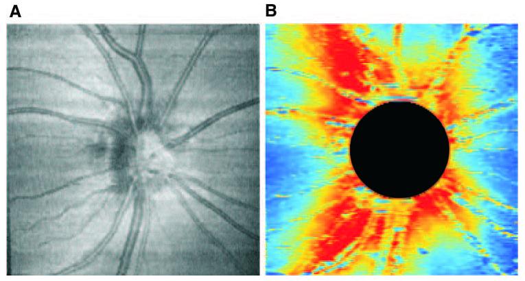
(A) hsUHR-OCT en face fundus image. (B) RNFL thickness map. Red: increased RNFL thickness; blue: decreased thickness. The ONH region (circle) was excluded from RNFL analysis.
Image Analysis
We developed a custom software program to segment the RNFL automatically, based on detection of the internal limiting membrane and outer RNFL border in each A-scan of each OCT frame. A perfect circle was subjectively fit to the disc margin on the hsUHR-OCT fundus image by an experienced operator (MG). We used a perfect circle to ensure that an identical number of sampling points were averaged when creating a profile line for a given segment on a given subject, as discussed later. RNFL thickness data outside of the region defined by this circle were used for the analysis and a color-coded RNFL thickness map was created (Fig. 1B). RNFL thickness information was then divided into inferior, superior, nasal, and temporal quadrants (90° each) as well as 12 segments of 30° (clock hours). Within each segment (quadrant or clock hour), average thicknesses at corresponding radial distances from the center of the ONH were calculated so that each segment could then be represented by a single-thickness profile line (average intrasubject profile). Each quadrant was composed of 240 radial lines, and each clock hour was composed of 80 lines. Since the raster scan consisted of 512 × 180 samples, oversampling in the y direction was required before creating these radial lines. Each radial line within a quadrant/clock hour for a given subject had the same length, which depended on the number of sample data points available. The shortest radial line in a given quadrant/clock hour represented the length of all the radial lines for that quadrant/clock hour. The thickness profile line for a given quadrant (or clock hour) was the average of 240 (or 80) radial lines, and a perfect circle was chosen to represent the ONH region to ensure that all points making up the profile line were based on an average of 240 (or 80) points. Thus, since the lengths of all radial lines in a given quadrant (or clock hour) were the same, a consistent number of samples were averaged to create the thickness profile line. If a perfect circle was not used to demarcate the ONH in this analysis, the length of the radial lines would be different, and thus the profile line would not be equally represented. The thickness measurements per quadrant and clock hour were also calculated at a distance of 1.7 mm from the disc center corresponding to the location of RNFL thickness measurements provided by the commercially available OCT (Stratus OCT; Carl Zeiss Meditec).
To ensure that a sufficient number of data points were present for the profile analysis, clock hour segments were excluded if the average intrasubject profile did not extend at least 200 pixels (∼2.4 mm) from the center of the ONH, which could occur if a disc was off-center during scanning. Mean RNFL thickness profiles for the entire study population, at each quadrant and clock hour, were averaged, and the region in which all qualified subjects had measurements was plotted (average intersubject profile). This method ensured that all profile lines were equally represented by all available subjects.
To investigate the decaying portion of RNFL profile, thickness measurements for each subject for each quadrant were smoothed using a mean filter. The location of the distal edge of the most distal peak of RNFL thickness was subjectively identified along the profile. Thickness measurements distal to this location were used for this analysis. Thus, the decay portion of filtered RNFL data could start at a different location for each subject. The measurements were averaged for each quadrant and the region in which all qualified subjects had measurements was plotted. The slope of the RNFL thickness profile was computed for each subject and each sector from these data. A linear mixed-effects model was fitted to the profile slope as a function of radius from the disc center, taking into account clustering within subjects.22
To investigate the variation along the RNFL thickness profile among the entire study population, the variance at each radial point (±50 μm) was plotted for each quadrant's mean-filtered data. An area of stable measurements with low variability among subjects has a variance approaching zero.
All the analyses were also conducted when the RNFL profiles were aligned, such that they all began at the disc margin without taking into account distance from the disc center. This alignment was made to ensure that variability in disc size within the study group did not affect the tissue profiles.
Results
Twelve eyes of 12 healthy volunteers (7 male, 5 female; mean age, 37.9 ± 7.2 years, range, 23–45; mean axial length, 24.42 ± 0.83 mm, range, 22.89–25.57) were enrolled. Seven clock hour and two quadrant segments (of 144 total clock hours and 48 total quadrants), all from two eyes, had to be excluded because measurements did not extend at least 2.4 mm from the center of the ONH. Mean disc radius based on the circular definition of the disc margin was 1.2 ± 0.1 mm (disc radius range, 1.03–1.33 mm; mean disc area, 4.3 ± 0.7 mm2).
RNFL thickness profile graphs of all quadrants and clock hours are shown in Figure 2. Thickness profiles in the superior, inferior, and temporal quadrants showed an initial increase in RNFL thickness, an area of peak thickness, and finally a decrease as radial distance from the center of the disc increased up to 2.5, 2.8, and 2.5 mm from the disc center, respectively. The nasal quadrant showed a consistent decrease in RNFL thickness up to a distance of 2.3 mm from the disc center. Three clock hour segments (2, 3, and 4 o'clock) did not exhibit an area of RNFL thickening and instead demonstrated a constant decrease in RNFL thickness only with increasing radius. The location of the scanning beam of the commercially available StratusOCT system is indicated on each profile (1.7 mm radius) and the thickness measurements are listed in Table 1. The overall mean RNFL thickness using StratusOCT was 103 and 153 μm using hsUHR-OCT, a difference of 50 μm between the two devices.
Figure 2.
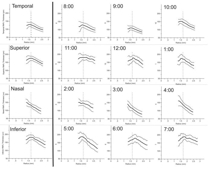
Quadrant (left) and clock hour (right) mean (solid line) and 95% confidence intervals (dotted lines) of nerve fiber layer thickness profiles in all subjects. Vertical dashed line: the location of the conventional OCT scan circle (1.7 mm from the center of the ONH).
Table 1.
Summary of Mean RNFL Thickness Measurements Taken at the Standard 3.4-mm Diameter with Stratus OCT and hsUHR-OCT
| Segment | Stratus OCT Mean RNFL Thickness (μm) |
hsUHR-OCT Mean RNFL Thickness (μm) |
|---|---|---|
| Overall | 103 | 153 |
| Temporal | 72 | 126 |
| Superior | 128 | 174 |
| Nasal | 79 | 131 |
| Inferior | 133 | 180 |
| Clock hour 1 | 113 | 168 |
| Clock hour 2 | 95 | 148 |
| Clock hour 3 | 63 | 113 |
| Clock hour 4 | 79 | 133 |
| Clock hour 5 | 115 | 184 |
| Clock hour 6 | 143 | 170 |
| Clock hour 7 | 140 | 186 |
| Clock hour 8 | 76 | 126 |
| Clock hour 9 | 56 | 107 |
| Clock hour 10 | 84 | 145 |
| Clock hour 11 | 140 | 180 |
| Clock hour 12 | 131 | 173 |
Similar profiles were observed for each participant. Aligning all profiles to the disc margin without taking into account the distance from the disc center produced profiles similar to those seen when distance was measured from the disc center (Fig. 3).
Figure 3.

A comparison of RNFL thickness profiles as measured from the center of the ONH (left) and from the disc margin (right).
Figure 4 shows a graph of average RNFL thickness in each quadrant after mean filtering. The inferior and superior quadrants showed the thickest RNFL and a very similar profile. In all four quadrants, the RNFL ultimately decayed linearly. A mixed-effects model (random intercepts) for the linear decay portion showed that the inferior, superior and nasal quadrant slopes were similar (−50.9, −53.7, and −53.2 μm/mm, respectively) but differed significantly from the slope in the temporal quadrant (−32.8 μm/mm; P = 0.0012, P = 0.0003, and P = 0.0004, respectively). These slopes and corresponding 95% confidence intervals can be seen in Table 2.
Figure 4.

Average nerve fiber layer quadrant thickness for all subject quadrants, after mean filtering.
Table 2.
Average Nerve Fiber Layer Thickness Decay Slopes and 95% CI in All Subjects
| Quadrant | Slope (μm/mm) (95% CI) |
|---|---|
| Inferior | −50.9 [−58.2-−43.6] |
| Superior | −53.7 [−61.4-−46.1] |
| Nasal | −53.2 [−60.8-−45.6] |
| Temporal | −32.8 [−40.1-−25.5] |
A graph of average variance between adjacent points in all four quadrants (after mean filtering of data in Fig. 4) can be seen in Figure 5. A high degree of variance was noted at the beginning of each profile, which corresponds to a region just outside of the disc margin, where major vessels are often present. The 1.7-mm location, or the location of RNFL thickness measurements provided by StratusOCT, is identified in Figure 4. This location corresponded to a region where variance was close to zero for the superior and inferior segments, whereas the variance in the temporal quadrant approached zero at a radius of approximately 1.55 mm. The point where the sum of all four variances was a minimum was 1.62 mm.
Figure 5.
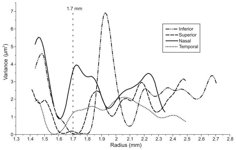
Average variance in nerve fiber layer thickness for all subjects after mean filtering. Superior and inferior quadrants are regions with more blood vessels, and a higher variability can be seen in these quadrants than in nasal and temporal quadrants. Vertical dashed line: location of the conventional OCT scan. The minimum total variance was observed at 1.62 mm from the disc center, which was close to the standard RNFL sampling location (1.7 mm; vertical dotted line) of the commercial OCT unit.
Discussion
This study evaluated the RNFL thickness profile in the peripapillary region of healthy subjects. Our findings showed thickening of the RNFL followed by a linear decay in the superior, inferior, and temporal segments and a constant linear decay in the nasal segment. These findings are in agreement with histologic measurements that were obtained from human and primate retinas.8-12 We also demonstrated that the circumpapillary scanning location used by OCT corresponds to an area of RNFL thickening near the minimum intersubject variability. This study is the first to describe this structure in living human subjects by hsUHR-OCT technology with a dense sampling of measuring points throughout the scanning area (sampling density, 2560 A-scans/mm2).
The current clinical standard for obtaining RNFL thickness measurements with StratusOCT is a peripapillary circular scan centered on the ONH with a radius of 1.7 mm. Measurements at this location have been shown to be the most reproducible compared with two other scan circles of different diameters.23,24 RNFL thickness measurements at this diameter have also shown high intrasession and intersession reproducibility in healthy25 and glaucomatous eyes in the commercially available device.26 However, the OCT scanning position was originally arbitrarily chosen to avoid intersecting tissue within the ONH margin in large discs and to avoid areas with peripapillary atrophy, but simultaneously to be close enough to the disc to allow a dense sampling covering the entire distribution of RNFL. Our data showed that in this cohort of healthy subjects at a distance of 1.7 mm from the disc center, the RNFL was thickest in the inferior, superior, and temporal segments. This is coincidentally the region of low thickness variability in the superior and inferior quadrants (Fig. 5). Thus, a decrease in the RNFL thickness in these thicker and more stable areas of the RNFL might be easier to detect. Measurements obtained from such locations would be more reproducible than in a constantly decaying region and would also be less prone to registration error. This is consistent with findings regarding reproducibility of OCT circumpapillary scans at various scan diameters.23
Mean RNFL thicknesses, shown in Table 1, were noticeably higher than those obtained with commercial time-domain OCT, probably because a different segmentation algorithm is used and the axial calibration of the hsUHR-OCT is different from the commercial device.
In the slope analysis, the nasal quadrant showed a slope that was similar to both the superior and inferior quadrants. However, the temporal quadrant showed shallower decay than the other quadrants (Fig. 4, Table 2), perhaps because the temporal RNFL bundle covers a narrower area in the retina and is a more dense structure than the other quadrants.
Findings similar to those reported herein were noted in each of the individual participants' profiles and when the RNFL profiles were aligned to the disc margin instead of the disc center (Fig. 3). Therefore, the pattern observed is not due to an averaging artifact but is instead due to tissue properties. This study was not designed to assess the effect of disc size on the RNFL profile and therefore further investigation is required to evaluate this effect.
Our findings agree with those of Skaf et al.,13 who created a profile of the RNFL using eight concentric circles around the ONH using StratusOCT. However, there are several limitations associated with the methods used in that study. Because the profile was created using only eight radial sampling distances, interpolation was necessary to fill in gaps between measurements. When considering the same retinal area used in our study (36 mm2), the number of thickness measurements in the study done by Skaf et al. was much lower than in our study (eight A-scans/mm2 vs the 2560 A-scans/mm2, respectively), as only nine points at each radial location (inferonasal, superonasal, superotemporal and inferotemporal) were used. In addition, data acquired using concentric circles with a separation of 0.2 mm are prone to eye motion artifacts during scanning with a slower time domain system. Processing of our three-dimensional data allowed virtual OCT fundus images to be created for our study. These images made it possible to exclude images in which large eye movements occurred and ensured there was a more accurate sampling registration.
The mean disc area in this study (4.3 ± 0.7 mm2) was larger than the commonly reported area, probably the result of forcing the disc margin to be defined by a perfect circle, thus overestimating the disc size in the temporal and nasal regions. The axial length range of subjects participating in this study was 22.89 to 25.57 mm. We did not use a magnification correction for the axial length because the range in this study had a negligible effect on the size of the scanning area (Piette S et al. IOVS 2002;43:ARVO E-Abstract 255) In addition, in a previous study in which OCT 2 was used, Bayraktar et al.27 found that in subjects with a wide range of axial lengths, the difference in RNFL thickness measurements before and after adjusting for magnification was less than the variability range inherent to the device. Therefore, for the range observed in our group, the effect was considered to be negligible.
The RNFL border-detection algorithm used in our study is influenced by neighboring measurements, and areas close to the ONH margin may have been affected due the rapid changes in RNFL at that location. Although data within the ONH region were excluded from analysis, the RNFL thickness profile measurement variability noted near the ONH margin and at the periphery in all quadrants and clock hours was most likely due to higher segmentation algorithm variability in these areas (Fig. 6). This algorithm also tended to overestimate the RNFL thickness when vessel shadows were present. The ONH margin often contained large blood vessels, and both the inner and outer RNFL borders had rapid contour changes (Fig. 6). This resulted in less reliable segmentation by the software in these specific locations. One other possible limitation of our study is the uneven sampling density of raster scanning since more axial scans were acquired in the horizontal direction (512 axial scans) than in the vertical (180 axial scans).
Figure 6.
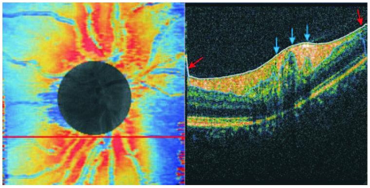
Algorithm failure. RNFL thickness map, where red marks the areas of the thicker RNFL and blue the thinner areas (left). The circle covers the ONH. A cross-sectional scan (right) was taken along the red line just under the disc margin. Red arrows: RNFL border detection algorithm failure toward the edge of the OCT image, where the signal was weaker. Blue arrows: an area just outside the ONH border where several blood vessels were located and the RNFL was thinner.
The orientation of the clock hours and quadrants followed straight radial lines in this study. Histologic data have shown that the RNFL orientation in the peripapillary region is mainly arcuate. We chose this pattern to simplify the analysis and to ascertain an identical size and number of measuring points in each segment. Future studies to investigate different patterns of analysis are warranted.
In conclusion, RNFL thickness is generally inversely related to the distance from the ONH center in the peripapillary region of healthy subjects, as determined with hsUHR-OCT. Aside from the nasal segment, all areas show an initial increase in RNFL, followed by a peak and a gradual linear decrease. In the nasal segment a linear decay appears without initial RNFL thickening.
Acknowledgments
Supported in part by National Eye Institute Grants R01-EY13178-06, R01-EY11289-20, P30-EY08098, and P30-EY13078; National Science Foundation Grants ECS-0119452 and BES-0522845; Air Force Office of Scientific Research Grant FA9550–040-1-0011; Medical Free Electron Laser Program Grant FA9550-040-1-0046; The Eye and Ear Foundation, Pittsburgh, PA, and an unrestricted grant from Research to Prevent Blindness, Inc.
Footnotes
Presented at the annual meeting of the Association for Research in Vision and Ophthalmology, Fort Lauderdale, Florida, May, 2006.
Disclosure: M.L. Gabriele, None; H. Ishikawa, None; G. Wollstein, None; R.A. Bilonick, None; L. Kagemann, None; M. Wojtkowski, None; V.J. Srinivasan, None; J.G. Fujimoto, None; J.S. Duker, None; J.S. Schuman, None
References
- 1.Hoyt WH, Frisen L, Newman NM. Fundoscopy of nerve fiber layer defects in glaucoma. Invest Ophthalmol Vis Sci. 1973;12:814–829. [PubMed] [Google Scholar]
- 2.Quigley HA, Miller NR, George T. Clinical evaluation of nerve fiber layer atrophy as an indicator of glaucomatous optic nerve damage. Arch Ophthalmol. 1980;98:1564–1571. doi: 10.1001/archopht.1980.01020040416003. [DOI] [PubMed] [Google Scholar]
- 3.Airaksinen PJ, Drance SM, Douglas GR, Mawson DK, Nieminen H. Diffuse and localized nerve fiber loss in glaucoma. Am J Ophthalmol. 1984;98:566–571. doi: 10.1016/0002-9394(84)90242-3. [DOI] [PubMed] [Google Scholar]
- 4.Sommer A, Katz J, Quigley HA, et al. Clinically detectable nerve fiber atrophy precedes the onset of glaucomatous field loss. Arch Ophthalmol. 1991;109:77–83. doi: 10.1001/archopht.1991.01080010079037. [DOI] [PubMed] [Google Scholar]
- 5.Hee MR, Izatt JA, Swanson EA, et al. Optical coherence tomography of the human retina. Arch Ophthalmol. 1995;113:325–332. doi: 10.1001/archopht.1995.01100030081025. [DOI] [PubMed] [Google Scholar]
- 6.Mainster MA, Timberlake GT, Webb RH, Hughes GW. Scanning laser ophthalmoscopy: clinical applications. Ophthalmology. 1982;89:852–857. doi: 10.1016/s0161-6420(82)34714-4. [DOI] [PubMed] [Google Scholar]
- 7.Weinreb RN, Shakiba S, Zangwill L. Scanning laser polarimetry to measure the nerve fiber layer of normal and glaucomatous eyes. Am J Ophthalmol. 1995;119:627–636. doi: 10.1016/s0002-9394(14)70221-1. [DOI] [PubMed] [Google Scholar]
- 8.Varma R, Minckler DS. Anatomy and pathophysiology of the retina and optic nerve. In: Ritch R, Shields MB, Krupin T, editors. The Glaucomas. 2nd ed. Mosby-Year Book, Inc.; St. Louis: 1996. pp. 139–151. [Google Scholar]
- 9.Radius RL. Thickness of the retinal nerve fiber layer in primate eyes. Arch Ophthalmol. 1980;98:1625–1629. doi: 10.1001/archopht.1980.01020040477018. [DOI] [PubMed] [Google Scholar]
- 10.Dichtl A, Jonas JB, Naumann GOH. Retinal nerve fiber layer thickness in human eyes. Graefes Arch Clin Ophthalmol. 1999;237:474–479. doi: 10.1007/s004170050264. [DOI] [PubMed] [Google Scholar]
- 11.Varma R, Skaf M, Barron E. Retinal nerve fiber layer thickness in normal human eyes. Ophthalmology. 1996;103:2114–2119. doi: 10.1016/s0161-6420(96)30381-3. [DOI] [PubMed] [Google Scholar]
- 12.Radius RL, Anderson DR. The course of axons through the retina and optic nerve head. Arch Ophthalmol. 1979;97:1154–1158. doi: 10.1001/archopht.1979.01020010608021. [DOI] [PubMed] [Google Scholar]
- 13.Skaf M, Bernardes AB, Cardillo JA, et al. Retinal nerve fibre layer thickness profile in normal eyes using third-generation optical coherence tomography. Eye. 2006;20:431–439. doi: 10.1038/sj.eye.6701896. [DOI] [PubMed] [Google Scholar]
- 14.Choma MA, Sarunic MV, Yang C, Izatt JA. Sensitivity advantage of swept source and Fourier domain optical coherence tomography. Opt Express. 2003;11:2183–2189. doi: 10.1364/oe.11.002183. [DOI] [PubMed] [Google Scholar]
- 15.Wojtkowski M, Srinivasan V, Fujimoto JG, et al. Three-dimensional retinal imaging with high-speed ultrahigh-resolution optical coherence tomography. Ophthalmology. 2005;112:1734–1746. doi: 10.1016/j.ophtha.2005.05.023. [DOI] [PMC free article] [PubMed] [Google Scholar]
- 16.de Boer JF, Cense B, Park BH, et al. Improved signal-to-noise ratio in spectral-domain compared with time-domain optical coherence tomography. Opt Lett. 2003;28:2067–2069. doi: 10.1364/ol.28.002067. [DOI] [PubMed] [Google Scholar]
- 17.Nassif N, Cense B, Park BH, et al. In vivo human retinal imaging by ultrahigh-speed spectral domain optical coherence tomography. Opt Lett. 2004;1(29):480–482. doi: 10.1364/ol.29.000480. [DOI] [PubMed] [Google Scholar]
- 18.Leitgeb RA, Hitzenberger CK, Fercher AF. Performance of Fourier domain vs. time domain optical coherence tomography. Opt Express. 2003;11:889–894. doi: 10.1364/oe.11.000889. [DOI] [PubMed] [Google Scholar]
- 19.Wojtkowski M, Srinivasan VJ, Ko TH, Fujimoto JG, Kowalczyk A, Duker JS. Ultrahigh-resolution, high-speed, Fourier domain optical coherence tomography and methods for dispersion compensation. Opt Express. 2004;12:2404–2422. doi: 10.1364/opex.12.002404. [DOI] [PubMed] [Google Scholar]
- 20.Wojtkowski M, Srinivasan V, Ko T, et al. High speed, ultrahigh resolution retinal imaging using spectral/Fourier domain OCT. Conf Lasers Electrooptics. 2005;3:2058–2060. [Google Scholar]
- 21.Mujat M, Chan R, Cense B, et al. Retinal nerve fiber layer thickness map determined from optical coherence tomography images. Opt Express. 2005;13:9480–9491. doi: 10.1364/opex.13.009480. [DOI] [PubMed] [Google Scholar]
- 22.Pinheiro JC, Bates DC. Mixed-Effects Models in S and S-Plus. Springer; New York: 2000. [Google Scholar]
- 23.Schuman JS, Pedut Kloizman T, Hertzmark E. Reproducibility of nerve fiber layer thickness measurements using optical coherence tomography. Ophthalmology. 1996;103:1889–1898. doi: 10.1016/s0161-6420(96)30410-7. [DOI] [PMC free article] [PubMed] [Google Scholar]
- 24.Carpineto P, Ciancaglini M, Zuppardi E, Falconio G, Doronzo E, Mastropasqua L. Reliability of nerve fiber layer thickness measurements using optical coherence tomography in normal and glaucomatous eyes. Ophthalmology. 2003;110:190–195. doi: 10.1016/s0161-6420(02)01296-4. [DOI] [PubMed] [Google Scholar]
- 25.Paunescu LA, Schuman JS, Price LL, et al. Reproducibility of nerve fiber thickness, macular thickness, and optic nerve head measurements using StratusOCT. Invest Ophthalmol Vis Sci. 2004;45:1716–1724. doi: 10.1167/iovs.03-0514. [DOI] [PMC free article] [PubMed] [Google Scholar]
- 26.Budenz DL, Chang RT, Huang X, Knighton RW, Tielsch JM. Reproducibility of retinal nerve fiber layer thickness measurements using Stratus OCT in normal and glaucomatous eyes. Invest Ophthalmol Vis Sci. 2005;46:2440–2443. doi: 10.1167/iovs.04-1174. [DOI] [PubMed] [Google Scholar]
- 27.Bayraktar S, Bayraktar Z, Yimaz OF. Influence of scan radius correction for ocular magnification and relationship between scan radius with retinal nerve fiber layer thickness measured by optical coherence tomography. J Glaucoma. 2001;10:163–169. doi: 10.1097/00061198-200106000-00004. [DOI] [PubMed] [Google Scholar]