Bayesian Mapping of Quantitative Trait Loci for Multiple Complex Traits with the Use of Variance Components

Abstract

Complex traits important for humans are often correlated phenotypically and genetically. Joint mapping of quantitative-trait loci (QTLs) for multiple correlated traits plays an important role in unraveling the genetic architecture of complex traits. Compared with single-trait analysis, joint mapping addresses more questions and has advantages for power of QTL detection and precision of parameter estimation. Some statistical methods have been developed to map QTLs underlying multiple traits, most of which are based on maximum-likelihood methods. We develop here a multivariate version of the Bayes methodology for joint mapping of QTLs, using the Markov chain–Monte Carlo (MCMC) algorithm. We adopt a variance-components method to model complex traits in outbred populations (e.g., humans). The method is robust, can deal with an arbitrary number of alleles with arbitrary patterns of gene actions (such as additive and dominant), and allows for multiple phenotype data of various types in the joint analysis (e.g., multiple continuous traits and mixtures of continuous traits and discrete traits). Under a Bayesian framework, parameters—including the number of QTLs—are estimated on the basis of their marginal posterior samples, which are generated through two samplers, the Gibbs sampler and the reversible-jump MCMC. In addition, we calculate the Bayes factor related to each identified QTL, to test coincident linkage versus pleiotropy. The performance of our method is evaluated in simulations with full-sib families. The results show that our proposed Bayesian joint-mapping method performs well for mapping multiple QTLs in situations of either bivariate continuous traits or mixed data types. Compared with the analysis for each trait separately, Bayesian joint mapping improves statistical power, provides stronger evidence of QTL detection, and increases precision in estimation of parameter and QTL position. We also applied the proposed method to a set of real data and detected a coincident linkage responsible for determining bone mineral density and areal bone size of wrist in humans.

In QTL mapping studies, it is a common practice to collect data observations on multiple traits. Generally, QTLs are mapped for the traits by use of single-trait analyses (i.e., analyzing the traits separately and reporting the respective results), although many of these traits are correlated phenotypically and genetically. An alternative way of QTL mapping for these correlated traits is joint analysis, by which multiple traits are analyzed simultaneously under a unified genetic model. The advantages of joint analysis over single-trait analysis are twofold. First, joint analysis may increase the statistical power and precision of QTL mapping because it combines phenotype information from all the traits and takes into account the correlation (environmental and genetic) structure of the traits. Second, genetic mechanisms of QTLs on correlated traits can be probed directly through joint analysis. For example, we can dissect a portion of genetic variation and covariation among traits by localizing QTLs and testing whether the genetic correlation is due to pleiotropy (i.e., a QTL influencing multiple correlated phenotypes) or coincident linkage (i.e., closely linked distinct QTLs for different traits).

Several methods have been developed for QTL mapping with the use of joint analysis for multiple traits.^1–14 Among these, different types of traits have been investigated, such as multiple continuous traits with normal distribution,^{1,2,5–7,11,12} multiple discrete traits,^3,8 and mixtures of traits with different phenotype distributions.^4,8–10 These studies can be grouped into three broad categories according to the statistical methods adopted, each of which has its advantages and limitations.

The first method is based on the likelihood-ratio test.^1,7,8,10 A concern with this method is that increasing the number of traits may lead to a large number of unknown parameters in the model; thus, potential gains from joint analysis may be offset by the increased degrees of freedom of the test statistic.¹⁰ In this situation, joint analysis could be less powerful than single-trait analysis.¹⁴

The second method adopts a semiparametric approach based on generalized estimation equations,³ which can avoid the difficulties of full-likelihood methods and can have some advantages, such as avoidance of distribution assumptions and the ease and flexibility of model specification.³ This method was developed under the double-cross design for experimental populations; its performance in natural populations (such as humans) remains unclear, and its performance relative to that of the single-trait analysis is not yet known.

The third method is based on the dimension-reduction technique and involves the performance of principal-components analysis (PCA)² for multiple correlated traits. Analysis of the “super traits” generated via PCA requires little extra effort in comparison with single-trait analysis. However, joint analysis based on PCA may incur spurious linkage^12,15 and cause difficulties in the biological interpretation of study results.

In QTL mapping for multiple correlated traits, the Bayesian method represents another useful tool because of some of its distinct advantages over the above three methods, such as the ease of results interpretation; the inherent flexibility in handling more-complex models, various experimental populations, and various types of phenotypes; and the resultant ability to incorporate information from different sources.^16–18 The Bayesian approach has been successfully used for QTL mapping of a single trait.^{16,17,19–29} However, so far, little work has been done for multiple correlated traits under a Bayesian framework.¹¹ In particular, no Bayesian method has been developed for mapping QTLs underlying correlated traits of a mixture of quantitative and discrete traits.

In this article, under an identity-by-descent (IBD)–based variance-components model, we developed a multivariate version of the Bayes method for QTL mapping of multiple traits under different situations, such as with multiple quantitative traits and mixed types of traits in humans. In addition, we show how to distinguish pleiotropy from coincident linkage, using the Bayes factor (BF). Our proposed method is implemented through the Markov chain–Monte Carlo (MCMC) algorithm, in which two samplers, the Gibbs sampler³⁰ and the reversible-jump MCMC (RJ-MCMC),³¹ are employed to generate joint posterior distributions of all unknowns. We conducted two simulation experiments to evaluate the performance of our method. The results show that our joint-analysis method outperforms univariate analyses and performs well for QTL mapping of multiple correlated traits under various situations. In addition, we applied our Bayesian joint-mapping method to a set of real data on humans. The results show that the proposed method has practical significance in the human genetics field.

Methods

Bayesian Mapping for Multiple Continuous Traits

Statistical model

Suppose there are n individuals with observations on m continuous traits in an investigated population. For ease of presentation, we adopt a full-sib design without having records for parents in each family. We assume that parents in all families come from an outbred population, where the distribution of genotypes at each locus is in Hardy-Weinberg equilibrium and the alleles of all loci under study are in linkage equilibrium. The multivariate mixed model can be written as

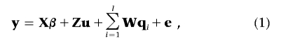where y=(y^′₁,…,y^′_k,…,y^′_n)^′ is an nm×1 vector of observations of n individuals on m traits (y_k is an m×1 vector of individual k on m traits), X is a design matrix, and β is a vector of fixed effects. In Bayesian theory, a “fixed effect” actually refers to the random effect with infinite prior variance, and its prior distribution is commonly assumed to be uniform with predefined upper and lower limits. Z is a design matrix relating records to individuals, u is a vector of additive polygenic effects, W is a matrix relating each individual’s record to its QTL effects, q_i is a vector of additive QTL effects corresponding to the ith QTL, and e is a vector of residuals. Here, we define l, the number of QTLs, as an unknown to be estimated. In model (1), suppose that the random vectors u, q_i, and e are mutually independent, each following multivariate normal distributions as follows:

where G is the m×m (co)variance matrix of the polygenic effects across m traits, A is the additive genetic relationship matrix that can be obtained from the pedigree of all individuals, and ⊗ is the Kronecker product operator.

where Q_i is the m×m (co)variance matrix of the ith QTL effects across m traits. Π_i is the IBD matrix for the ith QTL conditional on marker data (M) and the position (λ_i) of the ith QTL within the chromosome region considered. In this article, we use the IBD information of all markers simultaneously to infer IBD matrix Π_i, on the basis of the multipoint method proposed by Xu and Gessler.³²

where R is the m×m residual (co)variance matrix and I is an identity matrix.

Joint posterior distribution of parameters

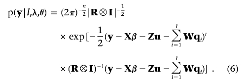
In a Bayesian framework, joint posterior distribution is the prerequisite to Bayesian inference. From model (1) and equations (2)–(4), parameters to be estimated include the number of QTLs, l; the locations of QTLs, ; and the model effects, θ=(β,u,q,G,Q,R) (here q denotes q₁,…,q_l, and Q denotes Q₁,…,Q_l). On the basis of the Bayes theorem, the joint posterior density of all parameters (l,λ,θ), conditional on the observables y, marker information M, and pedigree information A, can be written as

The first term in the right-hand side of equation (5) is the model’s likelihood conditional on all unknowns, which is assumed to be multivariate normal:

The second term in equation (5) is the joint prior distribution of (l,λ,θ), which can be extended as

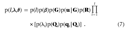The prior distributions of u and q_i are given in equations (2) and (3), respectively. The fixed effects β are random variables with uniform prior distributions on a predefined interval in the Bayesian framework:

The number of QTL, l, can be assumed to be a truncated Poisson distribution with mean μ_l and a predefined maximum L:

Since we have no information about QTL positions λ_i, a prior uniform distribution with an interval equivalent to the length of the chromosome region of interest is available for each QTL:

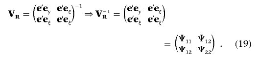
As for the prior distributions of G, Q_i, and R, we assume an m-dimensional inverted Wishart distribution with p df and an m×m scale matrix V for all these random matrices:

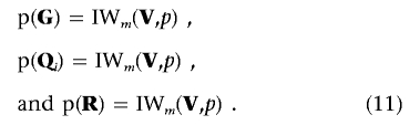If we have no prior knowledge about G, Q_i, and R, we can set V=0 and p=-(m+1), such that the distributions in equation (11) become uniform for these matrices.³³

Equations (2), (3), and (6)–(11) can together fully describe equation (5), the joint posterior distribution of all unknowns. This joint posterior is the basis for deriving the fully conditional distributions of all unknowns of interest, and further Bayesian inference for these unknowns will be based on respective fully conditional distribution via implementation of the Gibbs sampler and RJ-MCMC.

Fully conditional posterior distributions of unknowns

Following the basic idea of deriving the fully conditional distribution of a variable,³³ we pick up those terms that include this variable from the joint posterior distribution of all parameters given by equation (5).

Specifically, the fixed-effects vector β has a fully conditional distribution of

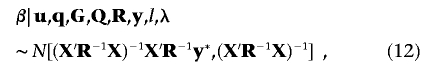where . The m×1 polygenic additive effects subvector, u_k(k=1,…,n), for individual k (with the assumption that each individual has observations on all m traits) has the form of the fully conditional distribution of

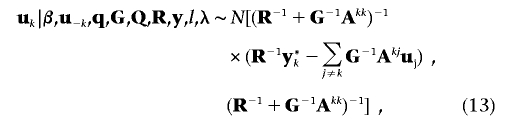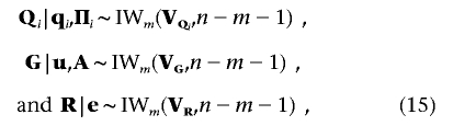
where . Here, X_k and W_k denote the respective matrices X and W with only the lines from (k-1)m+1 to km included, u_-k means the vector u with subvector u_k excluded, and A^kj is the (k,j)th element of the inverse of A. The fully conditional distribution of the m×1 effects subvector of the ith QTL, q_i,k(k=1,…,n), for individual k is given as

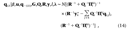where q_-(i,k) denotes vector q with the subvector q_i,k excluded, and . The fully conditional distributions of the (co)variance matrices Q_i(i=1,…,l), G, and R are m-dimensional inverted Wishart distributions, each having n-m-1 df:

where m×m scale matrices V_Qi, V_G, and V_R act as the hyperparameters of inverted Wishart distributions corresponding to the three random matrices. Here, the (r,s)th element of matrix V_Qi is V_Qi(r,s)=[q^′_i(r)Π^-1_iq_i(s)]^-1, with q_i(r) indicating the n×1 vector of the ith QTL effects for trait r(r=1,…,m). Similarly, the (r,s)th element of matrix V_G is V_G(r,s)=[u^′_(r)A^-1u_(s)]^-1, and the (r,s)th element of matrix V_R is V_R(r,s)=[e^′_(r)e_(s)]^-1, with e_(r) indicating the n×1 vector of environmental effects for trait r, where .

Unlike the above parameters, there is no explicit expression for the fully conditional posterior distributions of the parameters l and λ. Hence, we cannot obtain the kernel of a standard density—for example, normal distribution—for either of them. Accordingly, we use RJ-MCMC, an extension of the Metropolis-Hastings sampler,^34,35 to jointly draw the samples of these two parameters with no need for the explicit expressions of their fully conditional distributions (see detailed description in the following section).

Bayesian inference of unknowns based on MCMC process

We simulated an MCMC process for sampling the joint posterior distribution of all unknowns given in equation (5), and these joint posterior samples were used to perform Bayesian mapping and for parameter inference. The basic idea of the MCMC process is to mimic a random walk in the space of all unknowns in accordance with their respective fully conditional distributions. The simulated random walk finally converges to a stationary distribution,³⁶ which can be regarded as the joint posterior distribution of the unknowns.

When MCMC is performed, those unknowns except l and λ, each having the standard form of a fully conditional distribution, will be sampled through the Gibbs sampler, whereas changing the number of QTLs, l, requires a corresponding change in the dimension of the model and thus needs a reversible-jump step. This has been achieved via RJ-MCMC in suites of studies on single-trait QTL mapping.^16,17,28,29 In this article, we directly extend RJ-MCMC to sample the number of QTLs, l, and their positions, λ, in the case of multiple-trait mapping. Specifically, the MCMC process for generating the joint posterior samples of all unknowns can be briefly summarized as follows:

• 1. Initiate (l,λ,θ) in the space of all parameters with proper starting values in terms of their prior distributions given in equations (9) (l); (10) (λ); and (2)–(4), (8), (10), and (11) (θ).
• 2. Calculate IBD matrices for the corresponding QTLs in terms of their positions, using the multipoint method.³² Sample all unknowns included in θ in turn, in accordance with their fully posterior distributions given in equations (12)–(15).
• 3. Jointly sample l and λ, using the updating scheme similar to those in single-trait analyses,^16,17,28,29 in accordance with three types of moves with proposal probabilities p_m=1/3, p_d=1/3, and p_a=1/3 to (1) modify λ and keep l unchanged, (2) randomly remove one of the existing QTLs from the model if l>0, and (3) add a new QTL to the model if l<L, respectively.
  • a. 
    When the first type of move is chosen, we update positions for existing QTLs sequentially. Specifically, for the ith QTL, a proposal position λ^*_i is sampled from a uniform distribution with symmetric interval λ_i-d to λ_i+d around the previous position λ_i, where d is the predefined tuning parameter. The new vector of ith QTL effects, q^*_i, is also sampled from equation (14) in accordance with the IBD matrix Π^*_i corresponding to a new position λ^*_i. The proposal position λ^*_i is accepted with probability

    

    where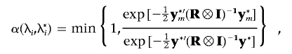 and . If the new position is accepted, the corresponding effect vector of the ith QTL, q^*_i, is also updated. Otherwise, both the position and effects of ith QTL remain unchanged. This sampling process will be repeated at the position of each existing QTLs.
  • b. 
    When p_d happens, each existing QTL has an equal probability of being removed from the current model. Suppose the ith QTL is proposed to be deleted; then, the multivariate version of acceptance probability is similar to single-trait mapping^37,38:

    

    where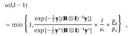 and . If the deletion of the ith QTL is accepted, the number of QTLs becomes l-1; otherwise, the previous value l remains unchanged.
  • c. 
    If the (l+1)th QTL is proposed to be added into the model, we will randomly assign starting values for corresponding parameters of the new QTL (λ_l+1, q_l+1, and Q_l+1), which is similar to step 1. When p_a happens, more QTL parameters with new starting values will be introduced to the model compared with single-trait mapping. To enhance the speed of convergence and to improve mixing of the Markov chain, we use the Gibbs sampler to perform more than one update of q_l+1 and Q_l+1 on the basis of alternating equations (14) and (15), before calculating the acceptance probability of adding a new QTL. In our studies, we empirically determine the extra 10 updates of parameters for the proposed QTL. Hence, the acceptance probability for the new QTL with updated parameters instead of their original starting values is given as

    

    where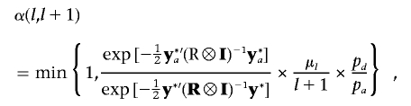 and . If the proposed QTL is accepted, the responding QTL parameters are also accepted, and the number of QTLs becomes l+1. Otherwise, the QTL number remains l.
• 4. The above steps constitute one iteration. The Markov chain will be constructed by repeating steps 2–3.

When large enough joint posterior samples of all unknowns are generated via the above MCMC process, QTL mapping and parameter estimation can be performed according to the marginal posterior density of all unknowns based on corresponding samples. Here, we adopt a histogram kernel to construct a QTL intensity function, which is used to determine the number and the locations of QTLs. Other parameters are also estimated from those samples in which QTL locations fall into the regions with sufficiently high estimated QTL intensities. This method has been commonly used in single-trait mapping.^{16,17,19,28,29}

Bayesian Mapping for Mixed Types of Traits

In practical research, investigators may collect data of different types for a sample set. For example, both binary traits (e.g., disease status) and continuous traits (e.g., quantitative measures that are risk factors for the disease under study) are available in a study. In this study, we describe—for the first time, to our knowledge—a Bayesian method for joint mapping of loci that affect the two different types of traits. We then derive a general version of the joint-mapping method for mixed types of multiple continuous traits and multiple ordered categorical traits.

Bivariate analysis with one binary trait and one continuous trait

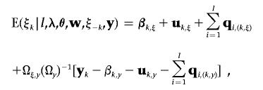
For a record in a binary fashion, an underlying normal variable, ξ_k, is often used to determine the value of w_k for individual k(k=1,…,n)—that is, w_k=1 if ξ_k>0, and w_k=0 if ξ_k⩽0. Because we set the threshold t=0, a constraint—that residual error variance σ²_e,ξ=1—must be superimposed to avoid overparameterization. From this threshold model, we can jointly analyze the continuous trait Y and the liability ξ on the basis of exactly the same methodology as the aforementioned Bayesian mapping for multiple continuous traits if only ξ is available. Hence, the key issue here is a need to generate the fully conditional distribution of the liability ξ. Following Sorensen’s method,³³ we can derive the fully conditional distribution of ξ_k for individual k:

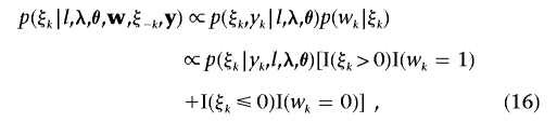where parameters l, λ, and θ have the same meanings as mentioned above; the n×1 vectors w=(w₁,…,w_n) and y=(y₁,…,y_n) contain phenotypic records for n individuals; and ξ_-k is the vector of liability ξ with ξ_k excluded. Note that p(ξ_k|l,λ,θ,w,ξ_-k,y) is a truncated (>0 if w_k=1 and <0 if w_k=0) normal distribution from equation (16). The mean of the conditional normal distribution of ξ_k is

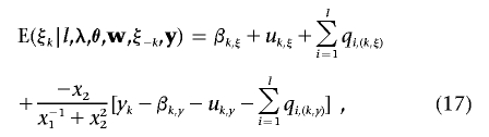and the variance is

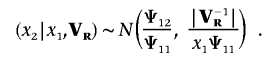
Here, the new parameters x₁ and x₂ are introduced for the drawing of samples of ξ, which are also used to update the (co)variance matrix of residual effects R between two traits.³³ A brief description of drawing samples of these two parameters is given below.

As mentioned earlier, we predefine the constraint σ²_e,ξ=1 because of the feature of binary data, rather than assigning an original inverse Wishart prior to [σ²_e,y, σ_e,yξ, σ²_e,ξ], as shown in equation (11). Accordingly, the 2×2 (co)variance matrix R between two traits has the form

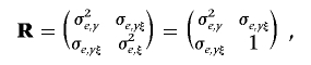which results in a conditional inverse Wishart prior to σ²_e,y,σ_e,yξ|σ²_e,ξ=1. Subsequently, the fully conditional distribution of σ²_e,y,σ_e,yξ|σ²_e,ξ=1,l,λ,θ,y,ξ follows a conditional inverse Wishart distribution. The parameters x₁ and x₂ can be used to indirectly sample σ²_e,y,σ_e,yξ from the conditional inverse Wishart distribution. For ease of presentation, we rewrite the scale matrix V_R in the inverse Wishart distribution given by equation (15):

First, we generate x₁ and x₂ by drawing successively from a one-dimensional Wishart distribution and a normal distribution, respectively:

and

Second, (x^-1₁+x²₂,-x₂) acts as a realized value from the fully conditional distribution σ²_e,y,σ_e,yξ|σ²_e,ξ=1,l,λ,θ,y,ξ. x₁ and x₂ jointly contribute to the updating of liability ξ through equations (17) and (18).

In brief, we need to make the following minor modification to the original MCMC process, to accommodate Bayesian mapping for a mixed type of bivariate analysis:

• 1. In step 1, we assign starting values to the liability ξ on the basis of the truncated normal prior.
• 2. In step 2, we generate x₁ and x₂ after updating the scale matrix V_R in equation (19), and then the liability ξ and the (co)variance matrix R are updated by x₁ and x₂. The original fully conditional distribution R|e∼IW_m(V_R,n-m-1) for sampling R will no longer play any role.

Except for the above two steps, no more modifications are required to construct the chain in joint analyses of mixed types of traits.

Additionally, we have extended the above methodology to a general situation in which multiple continuous traits and multiple ordered categorical traits are considered. A detailed description for this extension is provided in appendix A.

Testing Pleiotropy versus Coincident Linkage

In analyses of multiple traits, it is important to discriminate between pleiotropy and coincident linkage. In our studies, we developed a novel method that uses the BF to test for pleiotropy versus coincident linkage. For simplicity, we detail our method for bivariate analyses here.

For model (1) mentioned earlier in this section, we assume a pleiotropic QTL model—that is, l QTLs, each affecting all traits. Suppose we have detected a QTL within the chromosomal interval k_a to k_b with sufficient posterior density. To test pleiotropy versus coincident linkage, we propose a null model involving two closely linked QTLs within the interval k_a to k_b. It is reasonable that the covariance of QTL effects on the two traits can be constrained to 0.^6,10 Thus, testing pleiotropy versus coincident linkage is the comparison of the original pleiotropic model (model_plei.) with the coincident linkage model (model_link.), with use of the BF in a Bayesian framework.

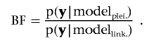The BF can be calculated via harmonic mean estimators³⁹ of the marginal probabilities, p(y|model_plei.) and p(y|model_link.), given the respective model.

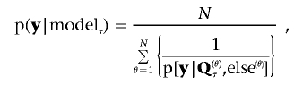where τ denotes either the pleiotropic model or the coincident linkage model fitted, and N is the number of total iterations in the MCMC process. Q^(θ)_τ and are samples of all unknowns drawn from the θth iteration. Here, Q_τ is the 2×2 (co)variance matrix of the QTL, which has been located in the interval k_a to k_b, and “else” denotes samples of all unknowns except Q_τ. Calculation of p[y|Q^(θ)_τ,else^(θ)] is straightforward according to equation (6).

Since calculation of the BF is based on the outcomes of original joint-mapping analyses, the estimates of QTL number and the CIs of respective QTLs will be treated as constant when pleiotropy versus coincident linkage is being tested via the BF, and we only need to update the location of each QTL and its respective parameters within its interval rather than add or delete a QTL via the reversible-jump step in the MCMC process. Furthermore, because the covariance of QTLs between two traits is constrained to 0 in the coincident linkage model, a simple conditional inverse Wishart distribution³³ is used to draw the samples of Q_τ under the null model, instead of using the original fully conditional distribution shown in equation (15).

On the basis of the output of the BF, we adopt the commonly used criteria^22,40 to judge which model—that is, pleiotropic or coincident linkage—is more favorable. Here, BF>10 and 10>BF>3 suggest a pleiotropic model with strong and moderate evidence, respectively. BF<0.1 and 0.1<BF<0.3 suggest a coincident linkage model with strong and moderate evidence, respectively. And, 0.3<BF<3 does not favor either model—that is, we cannot discriminate pleiotropic effects from coincidently linked QTLs within interval k_a to k_b.

Results

Simulation Studies

Design of the simulation experiments

To evaluate the proposed method, we conducted simulations for joint mapping of multiple traits in different scenarios. For conciseness, only two traits were considered in each of the two situations (two quantitative traits involved in the first simulation and a mixture of a quantitative trait and a binary trait in the second simulation). For ease of comparison, the same set of simulated data is used in both simulations, including the population, marker, QTL information, and phenotypic data.

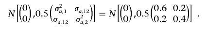
We simulated 1,000 full-sib families, each with 3 siblings (a total of 3,000 individuals). We assumed a chromosome region of 100 cM, with 11 evenly spaced codominant markers and an intermarker distance of 10 cM. Four alleles were randomly simulated with equal probability at each marker locus. Within the region, two sets of QTLs were simulated. The first set has two QTLs both residing at 25 cM, one with variance σ²_q1,1=0.2 for trait 1 and the other with σ²_q1,2=0.3 for trait 2; the covariance between two traits that is due to these two QTLs is σ_q1,12=0, which implies two coincidently linked QTLs. The second set has one QTL residing at 75 cM with parameters similarly defined as σ²_q2,1=0.2 for trait 1 and σ²_q2,2=0.3+ɛ for trait 2 and rendering covariance σ_q2,12=(σ²_q2,1×σ²_q2,2)^0.5 for the two traits, which implies a pleiotropic QTL. Here, we arbitrarily use a small positive constant, ɛ=0.01, to make the (co)variance matrix of the second QTL have the inverse. We set the polygenic (co)variances σ²_a,1=0.6, σ²_a,2=0.4, and σ_a,12=0.2 and residual (co)variances σ²_e,1=1.0, σ²_e,2=1.0, and σ_e,12=0 for the two traits.

In the first simulation experiment, normal distributed data of the two traits y₁ and y₂ for individual k(k=1,…,3,000) are generated using the infinitesimal model⁴¹:

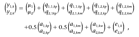where we take the overall mean vector (μ₁,μ₂)^′=(0,0)^′, and paternal- and maternal-allele effect vectors of the first QTL for individuals k,(q_1,1,kp,q_2,1,kp) and k,(q_1,1,km,q_2,1,km) are sampled from the same two-dimensional normal distribution with a 2×1 mean vector (0, 0)’ and a 2×2 variance matrix 0.5V_q1:

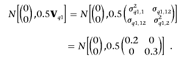Similarly, for the second QTL, vectors (q_1,2,kp,q_2,2,kp) and (q_1,2,km,q_2,2,km) are sampled from the same two-dimensional normal distribution with 2×1 mean vector (0, 0)’ and 2×2 variance matrix 0.5V_q2:

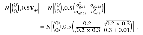The vectors (a_1,kp,a_2,kp)^′ and (a_1,km,a_2,km)^′ are paternal and maternal polygene additive effects vectors, respectively, which are sampled from

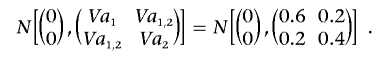The vector of within-family deviation in polygene effects (a_1,kw,a_2,kw)^′ is sampled from

The residual effect vector, (e_1,k,e_2,k)^′, is sampled from a two-dimensional standard normal distribution. On the basis of these two simulated observation vectors, we obtained the realized phenotypic (co)variance matrix,

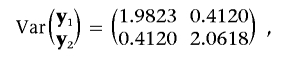which is highly consistent with the sum of all (co)variance matrices of all effects involved in the simulation.

In the second simulation experiment, we kept the original phenotypes of y₁ the same but truncated phenotypic values of y₂ to generate a new binary trait, w₂, using a threshold of 0. Because we set the overall mean to be 0 for both traits, this led to 50% population incidence for w₂.

To compare the efficiency of the joint analyses with single-trait analyses, separate analysis on each trait was also performed in the two simulation experiments. Our Bayesian mapping method for joint analyses can be directly used for single-trait analyses by taking the trait number m=1. In both experiments, we assume that phenotype records are not available for all the parents.

In each MCMC analysis, we ran a single long chain. We set the burn-in iterations to 1,000, and then the next 5×10⁵ cycles of simulations were performed to generate samples of all unknowns. We stored one iteration in every 50 MCMC cycles to reduce serial correlation between the samples, so that the total number of samples kept in each analysis was 10⁴. For each MCMC process, the initial values for all unknowns are randomly generated within the parameter space in accordance with their prior distributions, rather than with use of predetermined specific values. The prior for the overall mean was uniform over the range −2.0 to 2.0. The priors for all variance parameters were generated from the uniform range 0–2.0, and, for covariance parameters (only for joint analyses), the priors were generated from the range −2.0 to 2.0; the starting value for each (co)variance matrix must assure the existence of its inverse. We set the maximum number of QTLs as L=4 within the chromosomal region of 100 cM in length. The initial value of l was randomly sampled from its prior distribution given by equation (9). In addition, when we updated the location of the existing ith QTL, the tuning parameter of the proposal distribution, d_i, was set to 2 cM.

Results of the simulation experiments

The approximate Bayesian posterior distributions of QTL intensities obtained from both simulation experiments are presented in figure 1. The QTL intensity graphs corresponding to different analysis strategies, including joint mapping (denoted as J-12) and separate mapping for trait 1 (denoted as S-1) and trait 2 (denoted as S-2), are largely concentrated around the true locations of the two simulated QTLs. Specifically, when two continuous traits were considered in the analysis, two QTL intensity peaks (as shown in fig. 1a) were shaped on chromosomal positions of 24–25 cM and 75–76 cM for J-12, 24–25 cM and 76–77 cM for S-1, and 25–26 cM and 73–74 cM for S-2, whereas, when one continuous trait and one binary trait were involved in the analysis, two peaks (as shown in fig. 1b) were at 26–27 cM and 74–75 cM for J-12 and at 25–26 cM and 72–73 cM for S-2. (The graph for S-1 here is the same as that shown in fig. 1a because exactly the same data are adopted in both experiments.) Overall, all six graphs have two peaks that are quite close to the true positions of two QTLs. These results highly favor the two-QTL model, consistent with the cases in simulations. When comparing the shapes for J-12 with those for S-1 and S-2 in each experiment, all the highest QTL intensity peaks occurred in joint-mapping analyses, indicating that joint-mapping analyses provided stronger evidence and more information for QTL detection than did single-trait analyses. In addition, by comparing the shapes for J-12 in figure 1a and 1b, we found that some information was lost when binary data were involved in joint-mapping analyses. This is reflected by the result that the two QTL peaks for J-12 in figure 1b (for the mixture of one continuous trait and one binary trait) are less intense than those in figure 1a (for the two continuous traits).

Figure 1. .

Approximate posterior distributions of QTL locations based on QTL intensity with step length of 1 cM from joint mapping and single-trait mapping in both simulation experiments. a, Experiment 1 with two continuous traits. b, Experiment 2 with a mixture of one quantitative and one binary trait. J-12, S-1, and S-2 denote joint mapping for both traits and separate mapping for trait 1 and trait 2, respectively. The true number of QTLs is two, located at positions 25 and 75 cM.

The approximate posterior distributions of the QTL number generated from each analysis are presented in table 1. The posterior expectations, treated as estimates of the QTL number, are largely equal among different analyses and are consistent with the simulated number of QTLs. Furthermore, the posterior modes of the QTL number obtained from all analyses are the same as the true number of QTLs in both experiments. Within our expectation, the posterior variance of QTL number for multiple-trait analyses is smaller than those for single-trait analyses in both simulation experiments, and the variance of QTL number appeared smaller in the joint analysis for continuous traits than for mixed types of traits.

Table 1. .

Inferred Posterior Distribution and Posterior Mean of the Number of QTLs in Joint Mapping and Single-Trait Mapping from the Two Simulation Experiments

	Frequency
	No. of QTLs
Experiment and Method	0	1	2	3	4	Mean	Variance
1a:
J-12	.0002	.0054	.9928	.0012	.0004	1.9962	.0090
S-1	.0039	.0530	.8126	.1203	.0102	2.0799	.2233
S-2	.0009	.0616	.7989	.1320	.0066	2.0818	.2169
2b:
J-12	.0003	.0021	.9053	.0609	.0314	2.1210	.1752
S-1	.0039	.0530	.8126	.1203	.0102	2.0799	.2233
S-2	.0025	.0234	.8325	.1187	.0229	2.1361	.2252

^aIn the first experiment, two continuous traits, y₁ and y₂, are analyzed by joint mapping (J-12) and by separate mapping for y₁ (S-1) and y₂ (S-2).

^bIn the second experiment, the continuous trait y₁ and the binary trait w₂ are analyzed by joint mapping (J-12) and by separate mapping for y₁ (S-1) and w₂ (S-2).

Besides the estimate of QTL number given above, we also obtained estimates of all other unknowns involved in model (1) from respective posterior samples. The results from different simulation experiments, given in tables 2 and 3, are detailed below.

Table 2. .

Bayesian Estimates of Joint Mapping and Single-Trait Mapping from the First Simulation Experiment^[Note]

Analysis Methoda and Interval (∼cM)	Sum of the QTL Intensity	QTL Location (cM)	σ2qj,1	σ2qj,2	σqj,12	σ2a,1	σ2a,2	σa,12	σ2e,1	σ2e,2	σe,12	μ
J-12:						.5512 (.0146)	.3669 (.0180)	.1793 (.0101)	.9946 (.0095)	1.0704 (.0163)	.0590 (.0058)
20–28	.9940	24.3411 (2.2529)	.2138 (.0103)	.3170 (.0123)	−.0135 (.0019)							.0376μ1 (.0019)
72–81	.9976	75.5649 (2.0745)	.2288 (.0146)	.2947 (.0132)	.2360 (.0071)							.0251μ2 (.0016)
S-1:						.8307 (.1394)			.8992 (.0270)			.0401μ1 (.0044)
18–33	.8924	25.0136 (14.7105)	.1438 (.0304)
71–84	.9260	77.1874 (14.3854)	.1869 (.0322)
S-2:							.5325 (.0624)			.9813 (.0276)		.0286μ2 (.0030)
21–32	.9168	25.7168 (6.5950)		.2492 (.0336)
68–81	.9364	73.9050 (9.5818)		.2660 (.0296)

Note.— Both traits y₁ and y₂ are continuous. Posterior mean squared errors of the estimates are given in parentheses. σ²_qj,1, σ²_qj,2, and σ_qj,12 are the jth (j=1,2) QTL (co)variances of the two traits; σ²_a,1, σ²_a,2, and σ_a,12 are the polygenic (co)variances of the two traits; and σ²_e,1, σ²_e,2, and σ_e,12 are the residual (co)variances of the two traits.

^aJ-12 = joint mapping for traits y₁ and y₂; S-1 = separate mapping for trait y₁; S-2 = separate mapping for trait y₂.

Table 3. .

Bayesian Estimates of Joint Mapping and Single-Trait Mapping from the Second Simulation Experiment^[Note]

Analysis Methoda and Interval (∼cM)	Sum of the QTL Intensity	QTL Location (cM)	σ2qj,1	σ2qj,2	σqj,12	σ2a,1	σ2a,2	σa,12	σ2e,1	σe,12	μ
J-12:						.7806 (.0965)	.5270 (.0505)
23–33	.9848	26.3234 (5.9781)	.2364 (.0203)	.3389 (.0333)	−.0026 (.0040)			.2156 (.0111)	.9000 (.0211)	−.0128 (.0056)	−.0394μ1 (.0038)
69–79	.9658	74.4096 (2.3955)	.2103 (.0246)	.3472 (.0369)	.2277 (.0123)						−.0291μ2 (.0029)
S-1:
18–33	.8924	25.0136 (14.7105)	.1438 (.0304)
71–84	.9260	77.1874 (14.3854)	.1869 (.0322)			.8307 (.1394)			.8992 (.0270)		.0401μ1 (.0044)
S-2:							.6591 (.1982)				−.0343μ2 (.0050)
17–32	.9214	25.1521 (13.1565)		.3573 (.0595)
65–78	.8853	72.1356 (21.4333)		.4044 (.0916)

Note.— The continuous trait y₁ and the binary trait w₂ are considered in the analysis. Posterior mean squared errors of the estimates are given in parentheses. σ²_qj,1, σ²_qj,2, and σ_qj,12 are the jth (j=1,2) QTL (co)variances of the two traits; σ²_a,1, σ²_a,2, and σ_a,12 are the polygenic (co)variances of the two traits; and σ²_e,1, σ²_e,2, and σ_e,12 are the residual (co)variances of the two traits.

^aJ-12 = joint mapping for traits y₁ and y₂; S-1 = separate mapping for trait y₁; S-2 = separate mapping for trait w₂.

For all analyses in the two experiments, we chose a suitable length of a chromosomal region around each QTL intensity peak as the location interval of the detected QTL, and, thus, the summed QTL intensity within the chosen region was sufficiently high. The posterior means of the QTL locations and the estimates of QTL (co)variances among traits were also obtained from the respective posterior samples, in which QTL locations fell into the chosen chromosomal region for each detected QTL. From the results shown in tables 2 and 3, we found that the QTL interval showed a smaller length but a higher summed QTL intensity for joint mapping compared with separate mapping in both simulations. This demonstrates that joint mapping can provide stronger evidence and produce better precision for QTL detection. From the posterior means and posterior mean squared errors of QTL locations, the estimated locations were very close to the corresponding simulated true ones. However, separate analyses usually generated larger posterior mean squared errors than did joint analyses.

Similarly, QTL (co)variance estimates were largely close to the true values simulated, and the larger posterior mean squared errors of QTL variances always occurred in single-trait analyses compared with joint analyses. Note that estimates of QTL covariance among traits are available only in joint mapping for both simulations. For the first simulated set of QTLs under the coincident linkage model, the estimates of respective QTL covariance are close to 0 for both experiments. For the second simulated set of QTLs with pleiotropic effects, the corresponding QTL covariance estimates accordingly suggest a high QTL-effect correlation (close to 1) between the two traits. The results presented here show that the genetic mechanism of QTLs can be preliminarily probed through the respective estimates of covariance. Moreover, appropriate statistical testing—for example, use of the BF—can be used to further discriminate coincident linkage from pleiotropy.

The estimates of the overall mean, the polygene (co)variances, and the residual (co)variances are also given in tables 2 and 3 for the two simulations. It is clear that the covariance estimates for polygene and residual effects between traits can be obtained only from joint analyses. It appears that the estimates of these parameters are largely around the simulated values. However, the estimates from joint analyses are much closer to the true parameters and have smaller posterior mean squared errors than do those from separate analyses in both experiments.

The results presented in tables 1–3 and figure 1 demonstrate that the developed multivariate version of Bayesian mapping performs well for multiple continuous traits as well as for a mixture of traits. Compared with separate analyses, our joint-mapping method can enhance the precision and power in QTL detection as well as in estimation of other parameters. Moreover, from simulation results, it appears that joint mapping for multiple continuous traits always outperforms that for a mixture of traits, probably because of information loss in binary phenotypic data.

In table 4, we present the estimates of the BF for testing pleiotropy versus coincident linkage in the two simulation experiments. We calculated the BF on the basis of the MCMC process, to test coincident linkage of two nonpleiotropic QTLs against pleiotropy of a common QTL. The test was performed for each interval region where the QTL had been found in the initial joint analysis. For the first experiment, two QTL intervals, one 20–28 cM and the other 72–81 cM, were considered. For the second experiment, the tests were conducted in the two regions, one 23–33 cM and the other 69–79 cM. According to the commonly used criteria for choice of model based on the BF,^22,40 both estimates of the BF for the first set of QTLs in the two simulation experiments are far less than 0.1, which indicates a much higher posterior probability for the coincident linkage model and provides strong evidence for accepting the hypothesis of coincident linkage of two nonpleiotropic QTLs within this interval. For the second set of QTLs, we obtain the BF values from both simulations, which are much larger than 10.0. This gives strong evidence favoring the hypothesis of the second set of QTLs having pleiotropic effects on both traits. On the basis of the results in table 4, we accept the hypothesis that there exists coincident linkage of two nonpleiotropic QTLs within the interval of the first set of QTLs and one QTL with pleiotropic effects within the interval of the second set of QTLs for both simulation experiments. These results are consistent with the simulated genetic mechanism for the respective QTLs.

Table 4. .

BF for Testing Pleiotropy and Coincident Linkage for the Two QTLs Detected by Joint Mapping in Both Experiments

Experiment and Detected QTL	Interval (cM)	BF (Modelplei. vs. Modellink.)
1a:
QTL 1	20–28	3.55×10−3
QTL 2	72–81	1.87×102
2b:
QTL 1	23–33	8.26×10−2
QTL 2	69–79	.49×102

^aExperiment 1 considered two continuous traits.

^bExperiment 2 considered one continuous trait and one binary trait.

To confirm our proposed joint-mapping method, the multiple continuous data set simulated in the first experiment was also analyzed using the program SOLAR,⁴² version 3.04. Figure 2 shows the LOD-score profiles for J-12, S-1, and S-2 along the chromosome. We can see that each LOD-score profile shows two peaks. These two peaks are at positions 25 cM and 76 cM for J-12, 24 cM and 77 cM for S-1, and 26 cM and 74 cM for S-2, all overlapping the true locations of the two simulated QTLs. Comparing the shapes of different LOD-score profiles, we found that the LOD-score profile for J-12 has the highest peaks among the three types of analyses. These results are consistent with those obtained using our Bayesian joint-mapping method. Finally, in the J-12 analysis, we ran SOLAR to test pleiotropy versus coincident linkage at the two peak positions. At position 25 cM, we were able to reject the hypothesis of complete pleiotropy with an extremely small P value (P₁=6.91×10^-9) while accepting the hypothesis of coincident linkage (P₀=.2305). At position 76 cM, we rejected the hypotheses of coincident linkage with a very small P value (P₀=5.87×10^-10) but accepted the hypothesis of complete pleiotropy (P₁=.3741). These results are also in agreement with those obtained by using our testing method based on the BF.

Figure 2. .

LOD-score profiles of QTL mapping from joint analysis of two continuous traits (J-12) and separate analysis for trait 1 (S-1) and trait 2 (S-2), with the use of SOLAR software. Two QTLs are simulated at positions 25 and 75 cM.

It is apparent from figures 1 and 2 that the QTL intensity curves are much narrower and the peaks are more precisely located close to the simulated true QTLs with our method than with SOLAR. In addition, to draw generalizations from the studies, we simply simulated 50 independent samples because of the high computational demands of the MCMC algorithm for simulation 1, on the basis of the same parameter settings. Although 50 replicates are not sufficient to accurately evaluate the statistical power, a general idea about the performance of our method can be obtained in this way. In each replicate, we claimed a QTL as “detected” if there was a remarkable QTL intensity peak around the “true” position. We present the average estimates for parameters of each QTL obtained from 50 replicates in all analyses. As presented in table 5, higher powers and fewer posterior mean squared errors were largely seen in the joint analyses.

Table 5. .

Average Estimates of QTL Parameters Obtained from 50 Replicates in Each Analysis of the First Simulation Study^[Note]

	Parameter Estimate
QTL and Analysis Method	Position (cM)	Vqtl	Power
1:
J-12:	24.5072 (2.6319)		1.00 (50/50)
Trait 1		.2307 (.0252)
Trait 2		.2856 (.0183)
S-1	26.1832 (9.1047)	.1659 (.0344)	.92 (46/50)
S-2	25.4635 (7.2281)	.2706 (.0375)	.98 (49/50)
2:
J-12:	75.6623 (2.7051)		1.00 (50/50)
Trait 1		.2086 (.0173)
Trait 2		.3120 (.0198)
S-1	75.3598 (8.7454)	.1795 (.0426)	.94 (47/50)
S-2	74.0064 (7.3095)	.2941 (.0373)	1.00 (50/50)

Note.— The averaged posterior mean squared errors over 50 replicates are given in parentheses.

Real-Data Analyses

Bone mineral density (BMD) is the primary predictor of bone strength and fracture risk.^43–45 Areal bone size (ABS) is also a significant determinator of bone strength and has shown independence in predicting fracture risk.^46–49 Both BMD and ABS have strong determination, with heritabilities >50% in human populations.^43–45 Studies show that BMD and ABS are genetically correlated and may share some genetic determination.⁴⁹

To identify genomic regions that harbor QTLs having common effects on BMD and ABS at the forearm, we recently performed a bivariate genomewide linkage scan in a large sample of 451 white pedigrees comprising 4,498 individuals (X. Liu, Y. Liu, J. Liu, Y. Pei, P. Xiao, H. Shen, J. Deng, R. R. Recker, H.-W. Deng, unpublished data). Our preliminary results demonstrated a suggestive signal at chromosome 7p15, which showed coincident linkage. To further validate our proposed method, we performed a bivariate linkage scan, using our method on the same real-data set. Here, we performed linkage analyses only on chromosome 7 (encompassing 21 genotyped microsatellite markers), where the highest linkage peak was observed. For ease of calculation, we picked 364 independent nuclear families, comprising 2,007 subjects, from the original sample set. The number of sibs ranges from 2 to 14 across the families, with an average of 5.5.

As we did in simulation studies, we conducted Bayesian mapping for the real-data set, using both univariate and bivariate analyses. The QTL intensity distributions obtained from joint analysis (for BMD and ABS) and from separate analyses for BMD and ABS are given in figure 3. A QTL intensity peak was obtained in each analysis (joint analysis and separate analyses), highly favoring a single-QTL model. Furthermore, the joint analysis of BMD and ABS suggested a chromosome region having common effects on both traits. However, as clearly shown in figure 3, it is difficult to identify the linkage to ABS by performing single-trait analysis, because of the modest genetic effects and, thus, the weak linkage signals. As expected, we benefited from joint analysis under this situation because it yielded a more intense peak than did separate analyses for BMD and ABS. To further differentiate pleiotropy versus coincident linkage, we calculated the BF on the chromosomal interval 43–44 cM, where the QTL intensity peak was obtained. A coincident linkage model was favored from the calculation of the BF (0.0891). Our findings herein from the use of the Bayes method are largely consistent with those from our earlier linkage studies that used variance-components analyses implemented in SOLAR.

Figure 3. .

QTL intensity distributions based on joint analysis and separate analyses for BMD and ABS of wrist on chromosome 7

We also obtained the estimates of the number of QTLs and other relative parameter estimates for both BMD and ABS (data not shown). Compared with separate single-trait analyses, the joint analysis showed less estimation variance for the QTL number, higher posterior probability for the interval of identified QTLs, and lower SEs of parameter estimation. The increased estimation accuracy of parameters and higher posterior QTL intensity in real-data analysis clearly indicate that Bayesian joint analysis renders advantages over separate analyses, which provides further evidence to support our findings demonstrated in simulation studies.

Discussion

In this study, a joint-mapping method was developed using the MCMC algorithm in a Bayesian framework. The proposed method can handle multiple continuous traits, as well as a mixture of continuous and discrete traits (such as disease status).

Our proposed method has significant practical importance for genetic mapping of human complex diseases, such as essential hypertension (MIM 145500), type 2 diabetes (MIM 125853), osteoporosis (MIM 166710), obesity (MIM 601665), etc. When we map disease-susceptibility genes, the disease status is recorded and is generally treated as a dichotomous trait in statistical analysis. Moreover, in practical studies, measures of some highly related quantitative traits (risk factors of the disease) are often measured. For example, BMD, a quantitative measure of bone mass, is often used to evaluate the risk of osteoporotic fracture. Joint mapping that uses information from various data types can essentially increase precision of parameter estimations and, thus, the chance of identifying disease-susceptibility genes. Most importantly, given that quantitative risk factors may not share 100% of genetic determination with disease outcomes,^50,51 joint analyses of disease and quantitative risk factors can identify those genes that are shared and that are distinct between these two different types of disease-related phenotypes.

We performed an MCMC process to generate the marginal posterior distribution of the parameters of interest, which is not used in other existing joint-mapping methodologies. Inference for all parameters is based on their respective posterior samples. Two types of simulation experiments were conducted to evaluate the performance of the proposed method. The results clearly demonstrate that, compared with the single-trait analysis, our method can identify QTLs with higher posterior probabilities and narrower intervals and can estimate unknowns with smaller posterior mean squared errors. These findings suggest that the Bayesian joint mapping introduced here can improve the precision of parameter estimation and produces stronger evidence to identify QTLs.

We adopted a Bayesian method and implemented the procedure, using the MCMC algorithm. This is different from other existing joint-mapping methods. We used the Bayesian MCMC approach because of the following obvious advantages in comparison with the commonly used likelihood-ratio test methods: (1) One problem with the traditional likelihood-ratio test is that it is not always easy to obtain maximum-likelihood estimators either by maximizing the likelihood or by using an iterative algorithm, such as expectation maximum. But, in a Bayesian framework, we can avoid making such an optimization for joint-mapping analysis. (2) The Bayesian MCMC approach allows us to directly measure the probability as the evidence of the identified QTL and respective interval, which makes it easier to compare our results with the results of other experiments. To our knowledge, no other existing statistical paradigm is able to do this. In contrast, the P values obtained from likelihood-ratio tests cannot be readily compared among different experiments. Furthermore, we often encounter the multiple-comparison problem in statistical tests, and it is still challenging to deal with several dependent tests. Bayesian inference has an obvious advantage over traditional frequentist approaches, in terms of multiple-comparison testing, in that degree of belief is quantified by the posterior probabilities. Therefore, one can avoid, to some extent, the potential illogical conclusions that arise from an simple “accept/reject” decision process.⁵² (3) In a Bayesian framework, estimates of all unknowns are obtained from their posterior distributions, and, thus, we can avoid the use of asymptotic approximation by employing Fisher information. (4) The Bayesian method can construct more-complicated models by incorporating multiple levels of randomness and combining information from different sources.

Joint mapping offers an opportunity to distinguish coincident linkage from pleiotropy. In this study, we successfully distinguished the coincident linkage model and the pleiotropic model by employing a BF method for Bayesian joint mapping. To confirm the results of our BF method, we used SOLAR to test pleiotropy versus coincident linkage on the basis of a likelihood-ratio test⁶ for two continuous traits that are simulated in the first experiment. The results from SOLAR are highly in agreement with those from our BF method. However, our method gives much better precision and resolution, as shown in figures 1 and 2. So far, a suite of methods have been developed for joint mapping, most of which^{1,5–7,10,53} were based on likelihood-ratio tests. Departing from those likelihood-ratio–based methods, we used the BF to distinguish coincident linkage from pleiotropic models. The BF automatically generates the posterior probabilities for each model. The major advantage of the BF method is that it does not rely on any asymptotic results, which is a must for the likelihood-based methods, and it can provide exact outcomes with any amount of information. The more information used, the higher the probability that the “best” model will be obtained.⁵⁴ Recently, Varona et al.⁴⁰ proposed a method that uses the BF to distinguish between linked and pleiotropic QTLs under the linear regression model. In their approach, they adopted a Gibbs sampler to compute the posterior distribution of the QTL location under the linkage model. However, it is not clear if this approach could be adapted to identify the coincidently linked QTLs residing in the same marker bracket.

In the MCMC process, efficiency of the two samplers—that is, the Gibbs sampler and RJ-MCMC—depends on the mixing property of the Markov chain, which in turn is determined by the sampling scheme adopted and the parameterization involved in the model. To ensure that the Markov chain can mix well, we improved our sampling scheme when conducting RJ-MCMC for joint mapping in both simulation experiments. Specifically, when determining the acceptance probability of adding a new QTL via RJ-MCMC, we used the Gibbs sampler to perform an extra 10 updates of parameters for the proposed QTL, which greatly accelerated the convergence of the Markov chain, as expected.

In our studies, we adopted a conservative approach to deal with the convergence of MCMC. That is, thinning and burn-in values for all MCMC analyses were set to 50 and 50,000 (1,000×50), respectively. Empirically, these values are much higher than what are probably needed to ensure convergence of MCMC. Furthermore, we ran ^CODA, a widely used R package, to perform formal convergence tests, using the method of Raftery and Lewis.⁵⁵ From the diagnostic results for the two simulations (data not shown), it is clear that dependence factors for all parameters are <5.0, which indicates that the thinning and burn-in values adopted herein are reasonable for ensuring the convergence of MCMC. As for RJ-MCMC output for the QTL parameters, we generated a time-series plot of the sampled points for the number of QTLs in each analysis rather than use a formal convergence test. This is a common practice in Bayesian mapping.^16,17,28,29 It also shows that the RJ-MCMC algorithm mixes well over the number of QTLs. In addition, we calculated autocorrelation coefficients for samples of each parameter by running ^CODA. By comparing the amount of autocorrelation for each chain of parameters between single-trait analyses and joint analyses, we found that higher autocorrelation often occurred in joint analyses. This further suggests that we should generate a longer chain of parameters to reach convergence with the increasing of the number of traits involved in joint analyses, although the length of 1×10⁵ is large enough in our studies.

In the RJ-MCMC process, the information about a QTL is totally lost when we delete this QTL from the model, which could influence the acceptance probability and the mixing behavior.⁵⁶ Recently, two promising methods proposed for addressing the problem of RJ-MCMC—a stochastic search variable selection (SSVS) approach^56,57 and a Bayesian shrinkage method^58,59—were proposed for Bayesian mapping in experimental populations. In the SSVS procedure, a mixture prior is adopted to explicitly make a probabilistic statement about the inclusion of a QTL, and the markers with significant effects can be identified as those with higher posterior probability included in the model. As for Bayesian shrinkage analysis, each marker or marker interval is assumed to be associated with a QTL. If a marker or marker interval is not associated with any QTL, the corresponding QTL effect will be forced to shrink toward zero. Both methods above can largely avoid the problems seen in RJ-MCMC. Given the potential advantages of these two methods over RJ-MCMC, we will pursue further studies to extend them to a random model, which involves QTLs having infinite alleles. Under such a model, each QTL has infinite genotypes, and the QTL effects may vary across different individuals. Hence, with shrinkage analysis, it is impossible to shrink the designated QTL effect to zero if there is no associated QTL. Similarly, in SSVS, it is hard to make a probabilistic statement about the inclusion of a QTL according to the QTL effect. As such, with variance-components analyses, it may be a natural way to perform Bayesian shrinkage and SSVS analyses based on QTL variances instead of QTL effects. To develop such an extension of the two methods to an infinite-allele model, substantial effort is still needed.

The presented method is a variance-components joint-mapping procedure, which means that the infinite-allele model is used and the (co)variances of QTLs and other random effects in the model are treated as parameters of interest. Our method is quite suitable for natural outbred populations, such as humans. This is because the number of alleles at the locus is generally unknown in natural populations. Although the biallelic model could be appropriate in most situations, it may cause potential bias in estimation if the true number of the QTL alleles exceeds two. Using the variance-components model, we only need to estimate the (co)variances of respective QTLs, regardless of the number of the QTL alleles, which substantially improves the robustness of the Bayesian joint-mapping method.

In the simulation studies, for the purpose of simplicity, we used only full-sib families to show the performance of our proposed method. It is straightforward to extend our method to complex pedigrees by using a general approach to calculate the IBD matrix related to each QTL. Such a general approach has been developed by many investigators.^42,60,61 In addition, although our proposed method is focused on linkage analyses, it can be naturally extended to multiple-trait fine mapping by using both linkage analysis information and linkage disequilibrium (LD) information if highly dense markers are studied. Generally, combining LD information and linkage analysis information can significantly improve the power and precision of QTL mapping. For this situation, the extra effort needed is to remove the original assumption that founder QTL alleles are unrelated, and IBD probabilities between the founder QTL alleles can be estimated through the existing well-developed methods.^62,63

In our analyses, we assumed no correlation between the residuals. However, we acknowledge that the residual correlation may have significant influence on QTL mapping in joint analysis. From the findings of Jiang and Zeng¹ and Allison et al.⁶⁴ in joint-mapping analysis, the greatest power increases usually occur when the QTL-induced correlation is opposite in sign to the correlation induced by residual factors. Our proposed method can directly handle multiple phenotypic data without any modification when correlated residuals are assumed. We will investigate the efficiencies of our Bayesian joint-mapping procedure under several scenarios of residual correlations in our future endeavors.

Appendix A: Joint Analysis with Multiple Continuous Traits and Multiple Ordered Categorical Traits

Assume m₁ normal continuous traits and m₂ ordered categorical traits, each having C_s(s=1,…,m₂) ordered categories delimited by C_s-1 thresholds (m=m₁+m₂). We denote y=(y^′₁,…,y^′_k,…,y^′_n)^′ as an nm₁×1 vector of observations with n individuals on m₁ continuous traits and w=(w^′₁,…,w^′_k,…,w^′_n)^′ and ξ=(ξ^′₁,…,ξ^′_k,…,ξ^′_n)^′ as nm₂×1 vectors of phenotypes and the unobservable liability of n individuals on m₂ discrete traits, respectively. We also denote t_c,s as the cth threshold for the sth discrete trait (c=1,…,C_s-1). Similarly, if liability vector ξ can be drawn from its fully conditional distribution in each iteration of the MCMC process, Bayesian mapping for mixed types of m₁+m₂ traits can be performed using the method for m continuous traits detailed above. Since discrete data considered here fall in more than two categories, we cannot predetermine the threshold value t_c,s as done for binary traits. Thus, no constraint is superimposed to the (co)variance matrix of residual effects among m₂ discrete traits. For convenience of explanation, we present the m×m (co)variance matrix R among all m₁+m₂ traits as

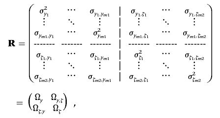where m×m matrix R is partitioned into four matrices—that is, an m₁×m₁ residual (co)variance matrix Ω_y among traits Y, an m₂×m₂ residual (co)variance matrix Ω_ξ among traits ξ, and an m₁×m₂ residual covariance matrix Ω_y,ξ between traits Y and ξ and its transpose, Ω_ξ,y.

According to the assumption of the threshold model,⁶⁵ it is straightforward to derive the fully conditional distribution of liability ξ_k for individual k:

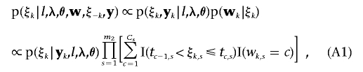where ξ_k,s and w_k,s are the sth elements in vectors ξ_k and w_k, respectively, for the sth discrete trait. w_k,s=c means that the observation on the sth discrete trait of individual k falls in category c. Specifically, t_0,s=-∞, t_Cs,s=+∞, and t_0,s<t_1,s<…<t_Cs,s for all s. In equation (A1), the fully conditional distribution of liability vector ξ_k is in the form of a truncated, conditional multinormal distribution; each element in ξ_k corresponding to categorical trait s is truncated at thresholds t_c-1,s and t_c,s. The mean vector of the truncated conditional multinormal distribution is given as

and the (co)variance matrix for the distribution is

Since we cannot predefine the thresholds for each categorical trait, the Gibbs sampler is also employed to generate those thresholds in the MCMC process, simply on the basis of a uniform distribution:

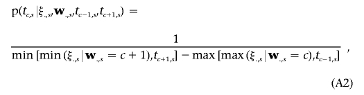where ξ_.,s and w_.,s denote subvectors of ξ and w related to categorical trait s. For each trait s(s=1,…,m₂), we successively draw the samples of all thresholds t_1,s,…,t_Cs-1,s in turn via equation (A2).

Compared with the original MCMC process for joint analyses with multiple continuous traits, additional efforts are needed for mixed types of traits considered here, including the following:

• 1. In step 1, we should assign proper starting values to thresholds of each categorical trait according to respective categories and then generate ξ in terms of threshold values t_c,s and w.
• 2. In step 2, the samples of t_c,s are drawn from equation (A2), followed by performance of the Gibbs sampler, to sample ξ on the basis of equation (A1). After that, the joint analysis with m₁ continuous traits and m₂ liability variables is essentially the same as that for m continuous traits.

References

- 1.Jiang C, Zeng ZB (1995) Multiple trait analysis of genetic mapping for quantitative trait loci. Genetics 140:1111–1127 [DOI] [PMC free article] [PubMed] [Google Scholar]
- 2.Weller JI, Wiggans GR, Vanraden PM, Ron M (1996) Application of a canonical transformation to detection of quantitative trait loci with the aid of genetic markers in a multi-trait experiment. Theor Appl Genet 92:998–1002 10.1007/s001220050221 [DOI] [PubMed] [Google Scholar]
- 3.Lange C, Whittaker JC (2001) Mapping quantitative trait loci using generalized estimating equations. Genetics 159:1325–1337 [DOI] [PMC free article] [PubMed] [Google Scholar]
- 4.Huang J, Jiang Y (2003) Genetic linkage analysis of a dichotomous trait incorporating a tightly linked quantitative trait in affected sib pairs. Am J Hum Genet 72:949–960 [DOI] [PMC free article] [PubMed] [Google Scholar]
- 5.Lund MS, Sorensen P, Guldbrandtsen B, Sorensen DA (2003) Multitrait fine mapping of quantitative trait loci using combined linkage disequilibria and linkage analysis. Genetics 163:405–410 [DOI] [PMC free article] [PubMed] [Google Scholar]
- 6.Almasy L, Dyer TD, Blangero J (1997) Bivariate quantitative trait linkage analysis: pleiotropy versus co-incident linkages. Genet Epidemiol 14:953–958 [DOI] [PubMed] [Google Scholar]
- 7.Knott SA, Haley CS (2000) Multitrait least squares for quantitative trait loci detection. Genetics 156:899–911 [DOI] [PMC free article] [PubMed] [Google Scholar]
- 8.Xu C, Li Z, Xu S (2005) Joint mapping of quantitative trait loci for multiple binary characters. Genetics 169:1045–1059 10.1534/genetics.103.019406 [DOI] [PMC free article] [PubMed] [Google Scholar]
- 9.Williams JT, Begleiter H, Porjesz B, Edenberg HJ, Foroud T, Reich T, Goate A, Van Eerdewegh P, Almasy L, Blangero J (1999) Joint multipoint linkage analysis of multivariate qualitative and quantitative traits. II. Alcoholism and event-related potentials. Am J Hum Genet 65:1148–1160 [DOI] [PMC free article] [PubMed] [Google Scholar]
- 10.Williams JT, Van Eerdewegh P, Almasy L, Blangero J (1999) Joint multipoint linkage analysis of multivariate qualitative and quantitative traits. I. Likelihood formulation and simulation results. Am J Hum Genet 65:1134–1147 [DOI] [PMC free article] [PubMed] [Google Scholar]
- 11.Meuwissen TH, Goddard ME (2004) Mapping multiple QTL using linkage disequilibrium and linkage analysis information and multitrait data. Genet Sel Evol 36:261–279 10.1051/gse:2004001 [DOI] [PMC free article] [PubMed] [Google Scholar]
- 12.Hackett CA, Meyer RC, Thomas WT (2001) Multi-trait QTL mapping in barley using multivariate regression. Genet Res 77:95–106 10.1017/S0016672300004869 [DOI] [PubMed] [Google Scholar]
- 13.Henshall JM, Goddard ME (1999) Multiple-trait mapping of quantitative trait loci after selective genotyping using logistic regression. Genetics 151:885–894 [DOI] [PMC free article] [PubMed] [Google Scholar]
- 14.Mangin B, Thoquet P, Grimsley N (1998) Pleiotropic QTL analysis. Biometrics 54:88–99 10.2307/2533998 [DOI] [Google Scholar]
- 15.Gilbert H, Le Roy P (2003) Comparison of three multitrait methods for QTL detection. Genet Sel Evol 35:281–304 10.1051/gse:2003009 [DOI] [PMC free article] [PubMed] [Google Scholar]
- 16.Yi N, Xu S (2000) Bayesian mapping of quantitative trait loci under the identity-by-descent-based variance component model. Genetics 156:411–422 [DOI] [PMC free article] [PubMed] [Google Scholar]
- 17.Yi N, Xu S (2000) Bayesian mapping of quantitative trait loci for complex binary traits. Genetics 155:1391–1403 [DOI] [PMC free article] [PubMed] [Google Scholar]
- 18.Dunson DB (2001) Commentary: practical advantages of Bayesian analysis of epidemiologic data. Am J Epidemiol 153:1222–1226 10.1093/aje/153.12.1222 [DOI] [PubMed] [Google Scholar]
- 19.Yi N, Xu S, George V, Allison DB (2004) Mapping multiple quantitative trait loci for ordinal traits. Behav Genet 34:3–15 10.1023/B:BEGE.0000009473.43185.43 [DOI] [PubMed] [Google Scholar]
- 20.Yi N, Xu S, Allison DB (2003) Bayesian model choice and search strategies for mapping interacting quantitative trait loci. Genetics 165:867–883 [DOI] [PMC free article] [PubMed] [Google Scholar]
- 21.Yi N, Xu S (2001) Bayesian mapping of quantitative trait loci under complicated mating designs. Genetics 157:1759–1771 [DOI] [PMC free article] [PubMed] [Google Scholar]
- 22.Satagopan JM, Yandell BS, Newton MA, Osborn TC (1996) A Bayesian approach to detect quantitative trait loci using Markov chain Monte Carlo. Genetics 144:805–816 [DOI] [PMC free article] [PubMed] [Google Scholar]
- 23.von Rohr P, Hoeschele I (2002) Bayesian QTL mapping using skewed Student-t distributions. Genet Sel Evol 34:1–21 10.1051/gse:2001001 [DOI] [PMC free article] [PubMed] [Google Scholar]
- 24.Uimari P, Hoeschele I (1997) Mapping-linked quantitative trait loci using Bayesian analysis and Markov chain Monte Carlo algorithms. Genetics 146:735–743 [DOI] [PMC free article] [PubMed] [Google Scholar]
- 25.Uimari P, Thaller G, Hoeschele I (1996) The use of multiple markers in a Bayesian method for mapping quantitative trait loci. Genetics 143:1831–1842 [DOI] [PMC free article] [PubMed] [Google Scholar]
- 26.Hoeschele I, Vanranden PM (1993) Bayesian analysis of linkage between genetic markers and quantitative trait loci. I. Prior knowledge. Theor Appl Genet 85:953–960 [DOI] [PubMed] [Google Scholar]
- 27.Hoeschele I, Vanranden PM (1993) Bayesian analysis of linkage between genetic markers and quantitative trait loci. II. Combining prior knowledge with experimental evidence. Theor Appl Genet 85:946–952 [DOI] [PubMed] [Google Scholar]
- 28.Sillanpaa MJ, Arjas E (1999) Bayesian mapping of multiple quantitative trait loci from incomplete outbred offspring data. Genetics 151:1605–1619 [DOI] [PMC free article] [PubMed] [Google Scholar]
- 29.Sillanpaa MJ, Arjas E (1998) Bayesian mapping of multiple quantitative trait loci from incomplete inbred line cross data. Genetics 148:1373–1388 [DOI] [PMC free article] [PubMed] [Google Scholar]
- 30.Chan JSK, Kuk AYC (1997) Maximum likelihood estimation for probit-linear mixed models with correlated random effects. Biometrics 53:86–97 10.2307/2533099 [DOI] [Google Scholar]
- 31.Green PJ (1995) Reversible jump Markov chain Monte Carlo computation and Bayesian model determination. Biometrika 82:711–732 10.1093/biomet/82.4.711 [DOI] [Google Scholar]
- 32.Xu S, Gessler DD (1998) Multipoint genetic mapping of quantitative trait loci using a variable number of sibs per family. Genet Res 71:73–83 10.1017/S0016672398003115 [DOI] [PubMed] [Google Scholar]
- 33.Sorensen D, Gianola D (2002) Likelihood, Bayesian and MCMC methods in quantitative genetics. Springer-Verlag, New York [Google Scholar]
- 34.Hastings WK (1970) Monte Carlo sampling methods using Markov chains and their applications. Biometrika 57:97–109 10.1093/biomet/57.1.97 [DOI] [Google Scholar]
- 35.Metropolis N, Rosenbluth AW, Rosenbluth MN, Teller AH, Teller E (1953) Equations of state calculations by fast computing machines. J Chem Phys 21:1087–1092 10.1063/1.1699114 [DOI] [Google Scholar]
- 36.Gelman A, Carlin JB, Stern HS, Rubin DB (1995) Bayesian data analysis. Chapman and Hall, London [Google Scholar]
- 37.Jannink JL, Fernando RL (2004) On the Metropolis-Hastings acceptance probability to add or drop a quantitative trait locus in Markov chain Monte Carlo-based Bayesian analyses. Genetics 166:641–643 10.1534/genetics.166.1.641 [DOI] [PMC free article] [PubMed] [Google Scholar]
- 38.Sillanpaa MJ, Gasbarra D, Arjas E (2004) Comment on “On the Metropolis-Hastings acceptance probability to add or drop a quantitative trait locus in Markov chain Monte Carlo-based Bayesian analyses.” Genetics 167:1037 [DOI] [PMC free article] [PubMed] [Google Scholar]
- 39.Kass RE, Raftery AE (1995) Bayes factors. J Am Stat Assoc 90:773–795 10.2307/2291091 [DOI] [Google Scholar]
- 40.Varona L, Gomez-Raya L, Rauw WM, Clop A, Ovilo C, Noguera JL (2004) Derivation of a Bayes factor to distinguish between linked or pleiotropic quantitative trait loci. Genetics 166:1025–1035 10.1534/genetics.166.2.1025 [DOI] [PMC free article] [PubMed] [Google Scholar]
- 41.Bulmer MG (1980) The mathematical theory of quantitative genetics. Oxford University Press, New York [Google Scholar]
- 42.Almasy L, Blangero J (1998) Multipoint quantitative-trait linkage analysis in general pedigrees. Am J Hum Genet 62:1198–1211 [DOI] [PMC free article] [PubMed] [Google Scholar]
- 43.Liu YJ, Shen H, Xiao P, Xiong DH, Li LH, Recker RR, Deng HW (2006) Molecular genetic studies of gene identification for osteoporosis: a 2004 update. J Bone Miner Res 21:1511–1535 10.1359/jbmr.051002 [DOI] [PMC free article] [PubMed] [Google Scholar]
- 44.Liu YZ, Liu YJ, Recker RR, Deng HW (2003) Molecular studies of identification of genes for osteoporosis: the 2002 update. J Endocrinol 177:147–196 10.1677/joe.0.1770147 [DOI] [PubMed] [Google Scholar]
- 45.Ralston SH, de Crombrugghe B (2006) Genetic regulation of bone mass and susceptibility to osteoporosis. Genes Dev 20:2492–2506 10.1101/gad.1449506 [DOI] [PubMed] [Google Scholar]
- 46.Augat P, Reeb H, Claes LE (1996) Prediction of fracture load at different skeletal sites by geometric properties of the cortical shell. J Bone Miner Res 11:1356–1363 [DOI] [PubMed] [Google Scholar]
- 47.Duan Y, Parfitt A, Seeman E (1999) Vertebral bone mass, size, and volumetric density in women with spinal fractures. J Bone Miner Res 14:1796–1802 10.1359/jbmr.1999.14.10.1796 [DOI] [PubMed] [Google Scholar]
- 48.Seeman E, Duan Y, Fong C, Edmonds J (2001) Fracture site-specific deficits in bone size and volumetric density in men with spine or hip fractures. J Bone Miner Res 16:120–127 10.1359/jbmr.2001.16.1.120 [DOI] [PubMed] [Google Scholar]
- 49.Deng HW, Xu FH, Davies KM, Heaney R, Recker RR (2002) Differences in bone mineral density, bone mineral content, and bone areal size in fracturing and non-fracturing women, and their interrelationships at the spine and hip. J Bone Miner Metab 20:358–366 10.1007/s007740200052 [DOI] [PubMed] [Google Scholar]
- 50.Deng HW, Mahaney MC, Williams JT, Li J, Conway T, Davies KM, Li JL, Deng H, Recker RR (2002) Relevance of the genes for bone mass variation to susceptibility to osteoporotic fractures and its implications to gene search for complex human diseases. Genet Epidemiol 22:12–25 10.1002/gepi.1040 [DOI] [PubMed] [Google Scholar]
- 51.Deng HW, Chen WM, Recker S, Stegman MR, Li JL, Davies KM, Zhou Y, Deng H, Heaney R, Recker RR (2000) Genetic determination of Colles’ fracture and differential bone mass in women with and without Colles’ fracture. J Bone Miner Res 15:1243–1252 10.1359/jbmr.2000.15.7.1243 [DOI] [PubMed] [Google Scholar]
- 52.Neath AA, Cavanaugh JE (2006) A Bayesian approach to the multiple comparisons problem. J Data Sci 4:131–146 [Google Scholar]
- 53.Cheverud JM, Routman EJ, Irschick DJ (1997) Pleiotropic effects of individual gene loci on mandibular morphology. Evolution 51:2006–2016 10.2307/2411021 [DOI] [PubMed] [Google Scholar]
- 54.Garcia-Cortes LA, Cabrillo C, Moreno C, Varona L (2001) Hypothesis testing for the genetic background of quantitative traits. Genet Sel Evol 33:3–16 10.1051/gse:2001107 [DOI] [PMC free article] [PubMed] [Google Scholar]
- 55.Raftery A, Lewis S (1992 ) How many iterations in the Gibbs sampler? In: Bernardo J, Berger J, Dawid A, Smith A (eds) Bayesian statistics. Oxford University Press, Oxford, United Kingdom [Google Scholar]
- 56.Yi N (2004) A unified Markov chain Monte Carlo framework for mapping multiple quantitative trait loci. Genetics 167:967–975 10.1534/genetics.104.026286 [DOI] [PMC free article] [PubMed] [Google Scholar]
- 57.Yi N, George V, Allison DB (2003) Stochastic search variable selection for identifying multiple quantitative trait loci. Genetics 164:1129–1138 [DOI] [PMC free article] [PubMed] [Google Scholar]
- 58.Xu S (2003) Estimating polygenic effects using markers of the entire genome. Genetics 163:789–801 [DOI] [PMC free article] [PubMed] [Google Scholar]
- 59.Wang H, Zhang YM, Li X, Masinde GL, Mohan S, Baylink DJ, Xu S (2005) Bayesian shrinkage estimation of quantitative trait loci parameters. Genetics 170:465–480 10.1534/genetics.104.039354 [DOI] [PMC free article] [PubMed] [Google Scholar]
- 60.Mao Y, Xu S (2005) A Monte Carlo algorithm for computing the IBD matrices using incomplete marker information. Heredity 94:305–315 10.1038/sj.hdy.6800564 [DOI] [PubMed] [Google Scholar]
- 61.Wang T, Fernando RL, Grossman M (1998) Genetic evaluation by best linear unbiased prediction using marker and trait information in a multibreed population. Genetics 148:507–515 [DOI] [PMC free article] [PubMed] [Google Scholar]
- 62.Meuwissen TH, Karlsen A, Lien S, Olsaker I, Goddard ME (2002) Fine mapping of a quantitative trait locus for twinning rate using combined linkage and linkage disequilibrium mapping. Genetics 161:373–379 [DOI] [PMC free article] [PubMed] [Google Scholar]
- 63.Meuwissen THE, Goddard ME (2001) Prediction of identity-by-descent probabilities from marker-haplotypes. Genet Sel Evol 33:605-634 10.1051/gse:2001134 [DOI] [PMC free article] [PubMed] [Google Scholar]
- 64.Allison DB, Thiel B, St Jean P, Elston RC, Infante MC, Schork NJ (1998) Multiple phenotype modeling in gene-mapping studies of quantitative traits: power advantages. Am J Hum Genet 63:1190–1201 [DOI] [PMC free article] [PubMed] [Google Scholar]
- 65.Falconer DS, Mackay TFC (1996) Introduction to quantitative genetics. Longmans Green Harlow, Essex, United Kingdom [Google Scholar]