Flexible Design for Following Up Positive Findings

Abstract

As more population-based studies suggest associations between genetic variants and disease risk, there is a need to improve the design of follow-up studies (stage II) in independent samples to confirm evidence of association observed at the initial stage (stage I). We propose to use flexible designs developed for randomized clinical trials in the calculation of sample size for follow-up studies. We apply a bootstrap procedure to correct the effect of regression to the mean, also called “winner’s curse,” resulting from choosing to follow up the markers with the strongest associations. We show how the results from stage I can improve sample size calculations for stage II adaptively. Despite the adaptive use of stage I data, the proposed method maintains the nominal global type I error for final analyses on the basis of either pure replication with the stage II data only or a joint analysis using information from both stages. Simulation studies show that sample-size calculations accounting for the impact of regression to the mean with the bootstrap procedure are more appropriate than is the conventional method. We also find that, in the context of flexible design, the joint analysis is generally more powerful than the replication analysis.

Replication is the sine qua non for establishing that a marker is truly associated with disease or phenotype.^1–3 Little attention, however, has been given to how to design a follow-up study (stage II) to validate findings for markers showing evidence of association at the initial stage (stage I) and how to interpret the results by use of information collected from both stages. This is particularly relevant because several studies seek to confirm their genetic associations with disease risk within large case-control and cohort consortia.

We face several related questions in designing a follow-up study. First, how can we exploit information from stage I to determine the effect size to be used in assessing the power? Here, we use the word “effect size” in the technical sense of a measure of the distance between an alternative hypothesis and a null hypothesis in terms of the chosen test statistic. To test a marker’s association with the disease risk, if a chosen test statistic (such as the likelihood-ratio test) has a noncentral χ² distribution under the alternative hypothesis, the effect size is the noncentrality parameter scaled by the sample size. It depends on both the magnitude of the hypothesized association parameter (e.g., odds ratio [OR]) and population parameters (e.g., genotype frequencies). The sample-size formula provides adequate power and efficient use of resource only if the effect size is appropriately assumed. For standard sample-size calculation, we usually assume an effect size rather arbitrarily, because little is known about the effect size in the study population before the stage I study. Data from stage I can lead to better estimation of the effect size.

Second, how do we combine the information from both stages for the final analysis? Statistical likelihood theory suggests that a test based on all the data is more powerful than any test of the same type I error level that looks at the components separately (if there is no genetic-effect heterogeneity between the two stages). But proper control of the type I error can be very difficult if the sample size for stage II is chosen adaptively—that is, is based on stage I results—because the distribution of the test statistic under the null in general is not easy to derive.

Finally, how do we decide stage II sample size to ensure adequate power for the final analysis? The sample-size calculation depends on the targeted effect size as well as the chosen test statistic mentioned above.

The typical way of choosing the effect size for the sample-size calculation in stage II is to assume the effect size seen in stage I. Because a marker is chosen for the follow-up study on the basis of its relatively large test statistic (small P value), the “observed” effect size is usually biased upward compared with its true value.^4–10 This is a classic example of the “regression to the mean”¹¹ or “winner’s curse”¹² effect. A statistic (or any measurement) chosen for replication because of an extreme observed value tends to be less extreme in the second study. The magnitude of the “regression to the mean” effect depends on the power of the stage I study, as well as the selection criteria for choosing markers for the follow-up study.⁹

Several methods have been proposed for correcting the bias in the observed effect size for linkage studies and population-based association studies.^5–9 For example, Zollner and Pritchard⁹ suggested a likelihood-based approach to estimate the effect size conditioned on observing a “significant” signal. Sun and Bull⁷ used the bootstrap procedure^13,14 to account for the selection bias in the observed genetic effect in linkage studies. Wu et al.⁸ examined the performance of the bootstrap estimate extensively in the linkage study of a quantitative trait. Here, we extend the method of Sun and Bull⁷ to estimate the effect size on the basis of the likelihood-ratio test. An additional advantage of the bootstrap approach for this problem is its applicability to general marker-selection criteria, including those based on rankings, not just to criteria based on P values.

In this article, we view the initial and follow-up studies as parts of a single flexible design.^15–17 Flexible designs were developed originally to minimize the number of participants needed in a randomized clinical trial by exploiting the limited data available in an interim analysis to determine final sample size. The sample size needed for stage II and the rejection region corresponding to the final analysis depends on the observed significance level of the stage I result. All parameters for stage I of a flexible design are set at the start, but some particulars of the second stage are determined by a prespecified analysis of data from the first stage. In contrast, the two phases in the standard two-stage design for genomewide association studies are designed before any stage I data are collected, and the information from stage I does not affect the design for stage II.^18–22

We adapt the flexible design approach of Proschan and Hunsberger¹⁶ to genetic association studies. First, we extend the technique to the general likelihood-ratio test, including the one based on the logistic-regression model that is most commonly used in association studies for the adjustment of nongenetic covariates. Scherag et al.²³ applied the idea of adaptive modification of sample size with an adaptive group sequential design²⁴ for the transmission/disequilibrium test²⁵ used in family-based studies. Second, to overcome the “regression to the mean” effect caused by marker selection criteria for the follow-up study, we use a bootstrap procedure similar to that recommended by Sun and Bull.⁷ We apply the proposed procedure to the design of a follow-up study to validate findings from a candidate-gene study²⁶ of non-Hodgkin lymphoma (NHL [MIM 605027]). We conduct simulation studies to evaluate the two-stage procedure’s conditional power and unconditional power.

Material and Methods

Problem Setup

In an association study, assume we have a stage I case-control sample of N₁ subjects. For each subject, we have the outcome y=1 for cases, y=0 for controls, nongenetic covariate q×1 vector X, and genetic covariates for M measured markers, where G_i is a d×1 vector coded for genotype at the ith marker. To assess marker i’s marginal effect on the outcome after adjustment for the effect of nongenetic covariates, we test each of the M null hypotheses Hⁱ₀:η_i=0, using the standard likelihood-ratio test, which compares the alternative model

against the null hypothesis

Denote the corresponding log-likelihood-ratio test statistic and associated P value for the ith marker as T_i and p_i, respectively. Given the testing results for individual markers from the existing stage I data, we want to identify a set of promising markers and design a follow-up study (called “stage II”) to further validate them.

An Adaptive Two-Stage Procedure

Commonly, investigators select markers with nominal stage I P values less than predetermined threshold α₁—for example, α₁=0.1—for further study. If no marker satisfies this criterion, they accept all null hypotheses Hⁱ₀,i=1,…,M, declare that all considered markers are not associated with the outcome, and do not consider a follow-up study. If, however, there are a total of f(f>0) markers with P values <α₁ at stage I, we propose to “adaptively” decide stage II sample size N₂ according to some rule Γ(D), which depends on stage I data D and, possibly, on other predetermined constraints and factors independent of D. Later, we suggest a specific sample-size determination rule Γ(D) based on the concept of conditional power.

Only markers with P<α₁ in stage I are selected for the follow-up study. We labeled the chosen markers , so their stage I P values satisfy p₁⩽p₂⩽…⩽p_f⩽α₁. For each marker i, 1⩽i⩽f, we perform the same likelihood-ratio test on the stage II data as in stage I and let the associated P value be q_i. We combine information from both stages with a final test statistic of the form

where is the standard normal distribution function and w is the predetermined weight for stage I, with 0⩽w<1, which is fixed and therefore independent of the stage I result. This is a commonly used method to combine P values from two independent tests.²⁷ For choosing the weight w, we can let w=0 or w=0.5. Following the terminology used by Skol et al.,¹⁸ we call the test statistic with w=0 the “replication-based test statistic” and the one with w>0 the “joint test statistic.”

At the end of stage II, the rejection region for each null hypothesis Hⁱ₀, 1⩽i⩽M, is , where c might be chosen to control the familywise type I error rate at the given α level. The value c is the solution, obtained numerically, to the equation

where z₁ and z₂ are independent random variables following the standard normal distribution. For any given marker i, p_i and q_i are independent, uniformly distributed random variables under the null hypothesis Hⁱ₀. The reason that p_i and q_i are independent is because q_i always follows the uniform distribution regardless of the stage II sample size. On the basis of equation (3), we have . Thus, under the global null hypothesis H^C₀=∩^M_i=1Hⁱ₀, the familywise type I error rate can be controlled at the level below α if c is chosen according to equation (3).

In summary, the adaptive two-stage procedure described above can be characterized by the parameters . It should be pointed out that the two-stage procedure always maintains its type I error rate regardless of the sample size decision rule .

Outline of Stage II Sample-Size Calculation

Once the set of candidate markers for stage II have been identified on the basis of stage I results, we want to calculate stage II sample size to ensure that we have appropriate power to detect disease-related markers. To calculate the sample size required to achieve this power, we need to identify a target marker among the set of chosen markers and to specify its effect size. We choose to focus on the top-ranked marker (marker 1, according to the notation above), which has a stage I P<α₁ and also is the marker with the smallest stage I P value among all studied markers, for the purpose of sample-size calculation. We do not claim that using the top-ranked marker is generally best, but we think it does assure us of a realistic power evaluation for the SNP that is most likely to be associated with disease. We consider alternative strategies in the “Discussion” section.

In the framework of the two-stage procedure described above, we have the freedom to adaptively choose stage II sample size without inflating the familywise type I error rate. To exploit this advantage, we can estimate the effect size and use it in the sample-size calculation. Below is an outline of steps for the sample-size calculation.

• Step 1. 

  Identify the set of follow-up markers and the top-ranked marker on the basis of stage I data, as mentioned above.

• Step 2. 

  Estimate the effect size of the top-ranked marker.

• Step 3. 

  Estimate the stage II sample size needed for the targeted conditional power with the effect size given by step 2 as the alternative hypothesis.

In the following sections, we describe steps 2 and 3 in detail.

Noncentrality Parameter and Effect-Size Estimation

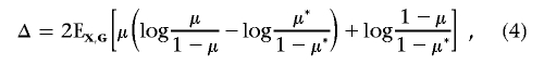
We first describe the noncentrality parameter, effect size, and their estimates for a single marker (without selection) and then describe the effect-size estimate for the top-ranked marker. Let G and X be the genetic and nongenetic covariates for the marker whose effect we are trying to replicate (here, we drop the index for the marker). As we mentioned above, to assess a given marker’s marginal effect, we can perform the association test based on the log-likelihood-ratio test statistic T, which compares two models given by equations (1) and (2). It is well known that T follows a central χ² distribution with d df if the marker is not associated with the disease. Under the alternative specified by model (1) with known , Self et al.^28,29 showed that T asymptotically follows a noncentral χ² distribution and provided a formula for calculating the corresponding noncentrality parameter λ. Shieh³⁰ simplified the calculation and suggested that the noncentrality parameter λ can be approximately calculated by λ≈N₁×Δ, where

with

and

Here, π^* and γ^* are estimated using the method of Self et al.²⁸ According to equation (3.2) in the article by Self et al.,²⁹ we have Δ=0 when η=0. Thus, the estimation for the noncentrality parameter is still valid when the null hypothesis is true (η=0).

For a marker that contributes to the disease risk described by model (1), we measure its effect size as Δ, defined by equation (4). The effect size Δ depends on the coefficients (ORs) specified in the risk model, as well as the joint distribution of in the study population. It is easy to see that the sample size required to detect the association between the marker and the disease for a given power and a type I error is directly proportional to 1/Δ. The larger the effect size, the smaller the required sample size.

Given the test statistic T, the noncentrality parameter λ can be estimated by

This estimate has smaller mean squared error than the standard maximum-likelihood estimate (MLE).³¹ The effect size Δ can be estimated from as

To design the follow-up study, we want to estimate the effect size for marker 1, the marker with lowest stage I P value, when its P value is below the marker selection threshold α₁. We can estimate its effect size Δ from the test statistic T₁ by use of formulas (5) and (6). This type of estimate, called the “naive estimate” by Sun and Bull,⁷ is often biased upward, because the marker is chosen for its extreme test statistic (small P value). In fact, T₁ does not follow the χ² distribution anymore. Sun and Bull⁷ explored a few approaches based on the bootstrap procedure to adjust the bias in the observed genetic effect.^13,14 Their simulation results suggest that a version analogous to the 0.632 estimator of Efron¹³ works generally well in a broad range of scenarios. The value 0.632 is the probability that a given subject will be selected at least once in a bootstrap sample. Here, we extend the method of Sun and Bull⁷ to estimate the effect size on the basis of the likelihood-ratio test. The basic steps are given in appendix A.

Stage II Sample-Size Calculation Based on Conditional Power

Once the effect size for the top-ranked marker has been estimated, we can calculate stage II sample size, using the concept of conditional power.¹⁶ Given the follow-up marker-selection threshold α₁ and the familywise error rate α, we decide on a rejection region , 1⩽i⩽M, by choosing the appropriate value for c based on equation (3). In fact, we need only to define S_i for i=1,…,f markers with observed stage I P<α₁.

For any given stage II sample size N₂, let T⁽²⁾_i be the likelihood-ratio test statistic for marker i based on stage II data. We can calculate the conditional power given the stage I result for detecting marker i (1⩽i⩽f) as

where the probability is defined under the true effect size Δ_i for marker i, and D represents all information collected at stage I, including, in particular, P values, τ(p_i), defined as

with χ²_d,1-τ being the 100(1-τ)th percentile of a central χ² distribution with d df. With the true effect size Δ_i, T⁽²⁾_i follows a noncentral χ² distribution with noncentrality parameter Δ_iN₂. From equations (7) and (8), we can see that τ(p_i) is the threshold for stage II P value q_i for selected marker i, 1⩽i⩽f. We would reject the null hypothesis Hⁱ₀ at the end if q_i<τ(p_i) and p_i⩽α₁.

For situations in which there is only one hypothesis, Proschan and Hunsberger¹⁶ suggested calculating N₂ to ensure a predetermined conditional power. Here, we decide to choose N₂ to achieve a specified conditional power 1-β for the detection of the top-ranked marker (marker 1). We can substitute the estimated (by the naive or bootstrap-based method) effect size for marker 1 into the calculation of the conditional power. The second stage sample size N₂ can be obtained by solving the equation

When τ(p₁)⩽1-β, the sample size N₂ is given by

where is the noncentrality parameter of a noncentral χ² distribution that has d df and its 100βth percentile equal to χ²_d,1-τ(p1) defined in equation (8). When τ(p₁)>1-β, since is an increasing function of , we have for any N₂>0 (under the assumption that the asymptotic distribution is still valid)—that is, there is no noncentral χ² distribution that has its 100βth percentile equal to χ²_d,1-τ(p1). In these situations, we can declare the association between the top-ranked marker and the outcome on the basis of stage I information alone and can base the sample-size calculation on the less significant markers.

When the replication-based test statistic is used—that is, w=0 in equation (8)—we have τ(p_i)=α/α₁, with p_i⩽α₁, which is independent of the stage I result. If we use the joint test statistic (such as w=0.5), τ(p_i) is a decreasing function of p_i—in other words, as p_i gets larger (i.e., there is less evidence against Hⁱ₀ from stage I data), a more stringent criterion is required for the stage II P value to reject Hⁱ₀ at the end of the two-stage procedure. In figure 1, we plot τ as a function of stage I P value for both joint and replication-based statistics. Parameters used in this example were α=0.01, M=40, and α₁=0.05. We can see that, given the same stage II sample size, the conditional power for the joint statistic is higher than that for the replication-based statistic when there is relatively strong evidence against the null (i.e., small P value) at stage I. On the other hand, when the evidence against the null is not very strong at the initial stage, the replication-based statistic tends to have higher conditional power than the joint test statistic does. Intuitively, this observation makes sense. Since the joint statistic combines information from both stages, a stage I P value far below α₁ increases the joint statistic value and makes it easy to reject the null hypothesis in the end. But a stage I P value just below α₁ requires stronger evidence from stage II for the final rejection of the null hypothesis than when the stage I P value is higher. Thus, the relative performance of joint and replication test statistics depend on the result from stage I. Neither one has uniformly better conditional power.

Figure 1. .

Threshold for the stage II P value for the rejection of final analysis as a function of stage I P value. The familywise type I error rate (α) is 0.01 with 40 independent hypotheses. The targeted conditional power (1-β) is 0.9. The marker selection criterion (α₁) is 0.05.

The Mean Conditional Power and “Unconditional” Power

When marker i^* is a true disease-associated marker, the “unconditional” power of the procedure specified by is the probability that marker i^* is among the chosen markers for follow-up and declared as significant at the end of stage II. Let TP represent the true-positive (TP) selection event , i.e., the event that marker i^* met the stage I criterion for carrying on to stage II, where D represents all information collected at stage I, we can express the unconditional power as

where all probabilities are defined under the alternative and is the expectation of the conditional power under the condition of a TP event, hereafter called the “conditional mean of the conditional power” (CMCP). Usually the power cannot be calculated analytically because it depends on the distribution of D and the complicated stage II sample-size decision rule Γ(D), although it can be evaluated empirically through simulation studies.

We can see from equation (9) that the power of the two-stage procedure depends on Pr(TP) and CMCP. As one might expect, we can increase the Pr(TP) at the cost of increasing stage I sample size and/or relaxing the marker-selection criterion by choosing a larger α₁. CMCP depends on stage II sample-size decision rule Γ(·). From the perspective of stage II design, we prefer a sample-size decision rule Γ(·) that has the CMCP close to its desired level, the target conditional power 1-β.

Application to NHL Study

Profound disruption of immune function is an established risk factor for NHL. Wang et al.²⁶ conducted a large-scale association study to evaluate common genetic variants in immune genes and their role in lymphoma. Cases were identified from four Surveillance, Epidemiology, and End Results (SEER) registries. Controls were identified by random-digit dialing and from Medicare eligibility files. Multiple SNPs from 36 candidate immune genes were genotyped. Their results suggested that perturbations in inflammation stemming from common genetic variants in proinflammatory cytokine genes TNF (MIM 191160) and LTA (MIM 153440) could contribute to the development of NHL.

We showed how our procedure might work in practice if we sought to calculate the sample size for stage II, using the study of Wang et al.²⁶ for stage I data. We wanted to design a follow-up study to validate and/or replicate findings of SNPs associated with the risk for the diffuse large B-cell lymphoma (DLBCL) subtype. Since most (>80%) of the subjects in the stage I study were whites (of European descent), we included only whites (318 patients with the DLBCL subtype and 766 controls) in the stage I data for this working example. A focus on whites allows comparisons of our results with those from the International Lymphoma Epidemiology Consortium (InterLymph),³³ a voluntary consortium established in 2000 to facilitate collaboration between epidemiological studies of lymphoma worldwide.

For the stage I data set, there were 48 informative SNPs. Each SNP was analyzed using a multiplicative model with adjustment for age (⩽54 years, 55–64 years, or ⩾65 years) and sex. The test for association was based on the likelihood-ratio test (with 1 df). Six SNPs had an observed P value <.05. A marker-selection criterion of α₁=0.1/48≈0.002 would identify two SNPs, rs1800629 and rs909253, for the follow-up study, with observed ORs of 1.54 and 1.40, respectively, on the basis of the multiplicative model. In table 1, we calculated the effect size and sample size required for each chosen SNP, using naive and bootstrap estimates for the targeted conditional power 1-β=0.9 and various familywise error rates: α=0.05, 0.01, or 0.005.

Table 1. .

Stage II Sample-Size Calculation for the NHL Example (DLBCL Subtype)

		Naive Estimation			Bootstrap Estimation
αa and SNPb	Pc	Effect Sized	N2 Replicatione	N2 Jointf	Effect Sized	N2 Replicatione	N2 Jointf
.05:
rs1800629	5.7 × 10−4	2.03	367	340	1.11	668	618
rs900253	7.4 × 10−4	1.93	386	378	1.01	740	725
.01:
rs1800629	5.7 × 10−4	2.03	844	821	1.11	1,536	1,495
rs900253	7.4 × 10−4	1.93	887	902	1.01	1,700	1,728
.005:
rs1800629	5.7 × 10−4	2.03	1,036	1,020	1.11	1,885	1,857
rs900253	7.4 × 10−4	1.93	1,088	1,117	1.01	2,086	2,141

^aα is the familywise type I error rate.

^bThe SNP chosen for the sample size calculation.

^cThe observed stage I P value.

^dEstimated effect size measured in units of 200 subjects.

^eSample size required when the replication-based test statistic is used with 1-β=0.9 and α₁=0.1/48. It is the total sample size for cases and controls combined. The ratio of case and control sample sizes remains the same as in stage I.

^fSample size required when the joint test statistic is used with 1-β=0.9 and α₁=0.1/48.

To estimate the effect size for the second-ranked SNP (rs909253), we removed the top-ranked SNP (rs1800629) from the data set and treated the second-ranked SNP as the “top-ranked” one observed in the remaining data. The same bootstrap procedure then can be applied to the remaining data set to estimate the effect size of rs909253. Preliminary simulation results suggested that using this strategy to estimate the effect size of the second-ranked marker still outperformed the naive method (results not shown).

For either SNP, the bootstrap estimated effect size was 46% less than the naive estimate (table 1). As a result, the sample size estimated by the naive method for stage II was just above half the sample size suggested by the bootstrap method. Simulation results (see section “Simulation Results: Effect-Size Estimates”) demonstrate that the bootstrap estimate, in general, is more accurate and precise than is the naive estimate. Thus, we recommend using the design based on the bootstrap estimate.

In addition to the effect size, we were also interested in OR estimation. The same bootstrap procedure was used to correct the bias in the naive estimate (based on MLE) of OR. The bootstrap-based OR estimates were 1.29 and 1.18 for SNPs rs1800629 and rs909253, respectively. They were much smaller than their original MLEs (1.54 and 1.40). We compared these estimates with the ORs reported by Rothman et al.,³³ who performed a pooled analysis restricted to whites within InterLymph. Rothman et al.³³ studied the association between 12 candidate SNPs (including rs1800629 and rs909253) and the risk of NHL (and subtypes) in whites. For the DLBCL subtype, there were >1,000 cases and 3,500 controls (about 25% of samples were from the study of Wang et al.²⁶) contributed from seven studies that had genotyped both SNPs. On the basis of the multiplicative model, with adjustment for age, sex, and study center, the estimated ORs for rs1800629 and rs909253 were 1.29 and 1.16, respectively, surprisingly close (and way too close than we should expect) to the 1.29 and 1.18 bootstrap estimates and much lower than the 1.54 and 1.40 naive estimates. Since the InterLymph pooled analysis was based on a large sample size, we expect its OR estimates to be accurate. Thus, it appears that the bootstrap estimate is more appropriate than is the naive estimate. This is consistent with simulation results (see section “Simulation Results: Effect-Size Estimates”).

Simulation Design

We conducted simulation studies to evaluate the performance of the bootstrap-based effect-size estimate and to investigate the size and conditional and unconditional power of the proposed adaptive two-stage procedure in the setting of typical candidate-gene association studies. We considered the following scenario to correspond to our NHL example. In a genetic association study of 41 candidate binary markers (SNPs), we collected either 300 or 500 cases and controls, with the number of controls always equal to the number of cases, from the study population at stage I. For simplicity, we assumed that all SNPs were independent (this assumption was not needed for the proposed procedure) and that only SNP 1 was associated with the disease through the disease-risk model

where x was a nongenetic dichotomous covariate with the value of 0 or 1 and g was the coded variable (under the assumption of a dominant model) for the disease-associated SNP with g=1 for genotypes having at least one copy of the risk-elevated allele and g=0 otherwise. For the analysis, we also assumed the dominant model. We let the OR exp(γ) for the nongenetic covariate x be 1.5 and varied the OR exp(η) for the disease-associated SNP among 1.3, 1.4, 1.5, and 1.6. The joint distribution of (x,g)in the general population was given as (0.4, 0.1, 0.35, 0.15) for (x=0, g=0), (x=0, g=1), (x=1, g=0), and (x=1, g=1), respectively. Given the joint distribution of (x,g), the OR, π, was chosen in such a way that disease prevalence was 0.1. Genotypes at a null marker were generated randomly (independent of case and control status) on the basis of a randomly chosen minor-allele frequency. For each stage I sample size (300 or 500 cases) and OR for the disease-associated SNP, we simulated 2,000 stage I data sets for the purpose of various performance evaluations.

Results

Simulation Results: Effect-Size Estimates

We compared the naive method with the bootstrap method for estimating the effect size of the top-ranked marker. We were interested only in evaluating their performances in situations when a TP selection was made—that is, when the disease-associated marker had a stage I P<α₁. If the disease-associated marker is not chosen for the follow-up study, the effect-size estimation has no implication for conditional power, since the conditional power is always zero in those situations.

For each simulated stage I data set with a TP selection, its top-ranked marker might or might not be the true disease-associated SNP. Table 2 summarizes the performance of two estimates in terms of bias and root mean squared error (RMSE) of the estimated effect size for each sample size and OR scenario. Results for effect-size estimation are measured in units of per 200 subjects—that is, we used 200Δ, with Δ as the estimated or true effect size. Results are stratified by whether the top-ranked SNP is the disease-associated or a null SNP. The “true” effect size for the disease-associated SNP is given by equation (4). The true effect size for a null marker is 0.

Table 2. .

Comparison of Bootstrap and Naive Methods for Estimating the Effect Size of the Top-Ranked Marker

	Disease-Associated Markere					Null Markerf
	Bias			RMSE		Bias			RMSE
N1, OR, Effect Size, and α1a	Proportiong	Naiveh	Bootstrapi	Naiveh	Bootstrapi	Proportiong	Naiveh	Bootstrapi	Naiveh	Bootstrapi
300:
1.3:
.67:
.05	.58	1.81	.73	2.08	1.08	.42	2.20	1.16	2.39	1.35
.5/41	.86	2.24	.99	2.42	1.28	.14	2.90	1.59	3.02	1.75
.2/41	.93	2.63	1.28	2.77	1.52	.07	3.29	1.84	3.33	1.90
.1/41	.96	3.05	1.62	3.15	1.82	.04	3.49	2.03	3.51	2.07
1.4:
1.11:
.05	.64	1.65	.52	2.09	1.21	.36	2.26	1.18	2.38	1.28
.5/41	.86	2.06	.80	2.38	1.37	.14	2.88	1.57	2.96	1.65
.2/41	.95	2.45	1.10	2.69	1.58	.05	3.29	1.86	3.35	1.92
.1/41	.97	2.88	1.46	3.07	1.87	.03	3.58	1.99	3.60	2.02
1.5:
1.66:
.05	.69	1.34	.17	1.93	1.28	.31	2.30	1.21	2.47	1.37
.5/41	.88	1.65	.39	2.11	1.34	.12	2.97	1.65	3.12	1.83
.2/41	.93	2.10	.75	2.45	1.51	.07	3.63	2.14	3.75	2.31
.1/41	.96	2.46	1.07	2.74	1.70	.04	3.99	2.43	4.08	2.55
1.6:
2.20:
.05	.76	1.11	−.08	1.94	1.53	.24	2.36	1.26	2.54	1.43
.5/41	.90	1.40	.13	2.06	1.54	.10	3.01	1.70	3.17	1.91
.2/41	.95	1.76	.42	2.28	1.61	.05	3.58	2.15	3.73	2.35
.1/41	.97	2.08	.71	2.51	1.73	.03	4.17	2.66	4.31	2.86
500:
1.3:
.67:
.05	.65	.84	.19	1.07	.59	.35	1.34	.69	1.42	.76
.5/41	.88	1.09	.35	1.26	.68	.12	1.72	.92	1.77	.97
.2/41	.94	1.38	.58	1.50	.84	.06	1.99	1.12	2.04	1.17
.1/41	.97	1.58	.75	1.69	.98	.03	2.32	1.38	2.36	1.41
1.4:
1.11:
.05	.71	.78	.07	1.20	.87	.29	1.40	.73	1.49	.81
.5/41	.87	.97	.21	1.31	.90	.13	1.75	.96	1.81	1.02
.2/41	.94	1.20	.39	1.47	.99	.06	2.07	1.18	2.10	1.23
.1/41	.96	1.41	.58	1.63	1.09	.04	2.19	1.29	2.22	1.34
1.5:
1.66:
.05	.81	.48	−.25	1.11	1.02	.19	1.44	.77	1.53	.85
.5/41	.91	.62	−.14	1.13	1.00	.09	1.78	.98	1.84	1.05
.2/41	.95	.82	.02	1.22	.99	.05	2.08	1.20	2.14	1.27
.1/41	.98	.98	.17	1.32	1.01	.02	2.34	1.42	2.38	1.47
1.6:
2.20:
.05	.86	.33	−.38	1.21	1.27	.14	1.47	.79	1.56	.88
.5/41	.94	.45	−.30	1.21	1.26	.06	1.85	1.04	1.92	1.13
.2/41	.97	.58	−.18	1.22	1.22	.03	2.10	1.23	2.16	1.30
.1/41	.98	.75	−.03	1.28	1.19	.02	2.41	1.48	2.46	1.54

^aN₁ is the number of cases at stage I. The numbers of cases is the same as the number of controls. The OR is for having the high-risk allele (a dominant model). Effect size is the true effect size for the disease-associated marker (measured in units of 200 subjects). α₁ is the P value threshold for follow-up marker selection.

^eResults are summarized over data sets that have a TP selection (i.e., the disease-associated marker has P<α₁) and that have the disease-associated marker as their top-ranked marker

^fResults are summarized over data sets that have a TP selection and that have a null marker as their top-ranked marker

^gProportion is the number of data sets with a TP selection whose top-ranked marker is the disease-associated (or null) marker divided by the number of data sets with a TP selection.

^hThe naive method was used for the effect-size estimation.

ⁱThe bootstrap method was used for the effect-size estimation.

When the top-ranked SNP is a null marker, the bootstrap estimate always has less bias and less RMSE than does the naive estimate. When the top-ranked SNP is the disease-associated marker, we can see from table 2 that the bootstrap estimate, in general, is more accurate and precise than is the naive estimate. The advantage of the bootstrap estimate is most obvious in situations where the effect size and/or sample size is relatively small. When the effect size is large (OR = 1.6) and the stage I sample size is 500 cases and 500 controls, the estimated bias and RMSE are comparable for both methods, though the estimate appeared slightly favorable compared with the naive method.

From the operational point of view, we are interested in the proximity between the estimate and the disease marker’s true effect size, regardless of whether the top-ranked marker is the disease-associated or null marker. Simulation results suggest that the bootstrap estimate is, in general, a better approximation (smaller RMSE) of the disease marker’s effect size than is the naive estimate (results not shown).

Simulation Results: Type I Error

We have shown that the “unconditional” familywise type I error rate can be controlled below α by use of the threshold c chosen by equation (3). Results on 40 independent null markers in simulated data sets can be used to see whether the false-positive rate is close to the nominal level. For each simulated stage I data set D, we identified the set of markers with their unadjusted P values <α₁. Let stage I P values for selected markers be p_i, 1⩽i⩽f. Similar to the power calculation given in equation (9), by assuming marker independency, we can calculate the “conditional” familywise error rate (condition on D) under the global null hypothesis H^C₀ as

where q_i is stage II P value and τ(p_i) is given by equation (8). If no marker can be selected from stage I, the “conditional” familywise error rate is 0. Thus, the familywise error rate can be estimated as the average “conditional” familywise error rate over all simulated data sets.

Simulation results are summarized in table 3. It is clear from the table that the familywise error rates for various α₁, α, and sample sizes are very close to their nominal levels. When there is linkage disequilibrium between markers, we expect that the actual type I error rate should be below its nominal level because of the conservative nature of the Bonferroni correction.

Table 3. .

Familywise Type I Error for Final Analyses

	Sample Size = 300				Sample Size = 500
	α=.01b		α=.05b		α=.01b		α=.05b
α1a	Jointc	Replicationd	Jointc	Replicationd	Jointc	Replicationd	Jointc	Replicationd
.05	.010	.010	.049	.050	.010	.010	.047	.048
.5/40	.010	.010	.049	.048	.009	.010	.047	.047
.2/40	.010	.009	.048	.047	.010	.009	.047	.046
.1/40	.011	.010	.049	.049	.010	.010	.049	.049

^aα₁ is the P value threshold for follow-up marker selection.

^bα is the nominal familywise type I error rate.

^cThe analysis is based on the joint test statistic.

^dThe analysis is based on the replication-based test statistic.

Simulation Results: Conditional Power

To evaluate the impact of different effect-size estimates on the design in terms of conditional power, we can compare their estimated CMCP defined in equation (9) and see which one is closer to the nominal level 1-β. Given a simulated stage I data set with a TP selection, its actual conditional power can be calculated analytically from equation (7) by use of the sample size estimated by either the naive or bootstrap method. We can empirically evaluate CMCP, using the average actual conditional power over simulated stage I data sets with a TP selection. In the simulation, we let the familywise type I error (α) be 0.01 and the target conditional power (1-β) be 0.9. In table 4, we provide the estimated CMCP for various sample sizes, ORs, and marker-selection criterion α₁. The results shown in table 4 are based on the joint test statistic (w=0.5). It can be seen from table 4 that the design using the bootstrap estimate has a CMCP closer to the target value (1-β=0.9 in this case) than that of the design using the naive estimate. This is also true for the replication-based test statistic (results not shown). Similar to the results shown in table 2, the advantage of using the bootstrap estimate is particularly striking when the effect size and/or sample size is relatively small. When the OR is 1.6 with a sample size of 500 cases and 500 controls, we notice from table 4 that the CMCP achieved using the bootstrap estimate is slightly higher than the target value, because of the underestimation of the effect size.

Table 4. .

Average Actual Conditional Power of Joint Analysis

	N1=300c		N1=500c
ORa and α1b	Naived	Bootstrape	Naived	Bootstrape
1.3:
.05	.31	.61	.54	.82
.5/41	.31	.56	.51	.78
.2/41	.34	.53	.50	.73
.1/41	.38	.53	.52	.70
1.4:
.05	.52	.79	.73	.90
.5/41	.50	.75	.71	.88
.2/41	.50	.72	.69	.85
.1/41	.52	.69	.68	.83
1.5:
.05	.70	.89	.85	.93
.5/41	.67	.87	.83	.93
.2/41	.65	.83	.81	.92
.1/41	.64	.80	.80	.91
1.6:
.05	.79	.92	.89	.94
.5/41	.77	.91	.88	.94
.2/41	.75	.89	.87	.93
.1/41	.74	.87	.86	.93

^aOR for having the high-risk allele (a dominant model).

^bα₁ is the P value threshold for follow-up marker selection.

^cN₁ is the number of cases at stage I. The number of controls is the same as the number of cases.

^dThe naive method was used for the effect-size estimation.

^eThe bootstrap method was used for the effect-size estimation.

We can stratify the results according to whether the top-ranked marker is the disease-associated marker. For both categories, the average actual conditional power by use of the bootstrap method is higher than that by use of the native method and is closer to the target level in most scenarios (results not shown).

Simulation Results: “Unconditional” Power

We evaluated the “unconditional” power of the two-stage procedure, using the joint statistic and bootstrap-based effect-size estimate. In figure 2, stratified by α₁, we plot the unconditional power against various target conditional powers ranging from 0.55 to 0.9. We show only the values for ORs of 1.3 and 1.6. Patterns for ORs of 1.4 and 1.5 were similar. From figure 2, we can see that the power increases as the marker selection criterion α₁ gets larger (i.e., less restrictive).

Figure 2. .

“Unconditional” power of the adaptive two-stage procedure by use of the joint statistic under various ORs and stage I marker selection criterion (α₁). The stage I sample size is 500 cases and 500 controls. The familywise error rate is controlled at 0.01 with a total of 41 independent hypotheses. For each simulated stage I data set, the marker with the lowest stage I P value is used for stage II sample-size calculation. Its effect size is estimated by the bootstrap method. Stage II sample size is calculated using the joint statistic for the corresponding target conditional power. The “unconditional” power is estimated according to formula (9) on the basis of 2,000 simulated stage I data sets.

Finally, we tried to make a direct comparison between the two-stage procedure that uses the joint statistic and the one that uses the replication statistic. To make a fair comparison, two procedures should use the same stage II sample-size decision rule. We chose the common rule based on the replication statistic with the bootstrap-estimated effect size. Results are shown in figure 3 for α₁=0.05 and 0.5/41, with ORs of 1.3 and 1.6. Patterns are similar for other α₁ levels and for ORs of 1.4 and 1.5 (results not shown). It is clear that it is generally more powerful to use the joint statistic in the two-stage procedure than to use the replication-based statistic in all considered scenarios.

Figure 3. .

“Unconditional” power comparison between the two-stage procedure using the joint statistic and that using the replication statistic (Repl.) under various ORs and stage I marker-selection criterion (α₁). The stage I sample size is 500 cases and 500 controls. The familywise error rate is controlled at 0.01, with a total of 41 independent hypotheses. For each simulated stage I data set, the marker with the lowest stage I P value is used for stage II sample-size calculation. Its effect size is estimated by the bootstrap method. The stage II sample size is calculated using the replication-based test statistic for the corresponding target conditional power. The same sample-size decision rule is applied to both procedures, to ensure a fair comparison. The “unconditional” power is estimated according to formula (9) on the basis of 2,000 simulated stage I data sets.

Discussion

An independent follow-up study is as integral to the establishment of true associations as is the original “discovery” study.^1–3 The design of these follow-up studies, however, may lead to underpowered studies if the optimistic estimate of the effect size from the primary study is used in the sample-size determination. We proposed to use the idea of a flexible design,^15–17 originally developed for randomized clinical trials, to determine sample size for the follow-up study adaptively based on results from stage I, while controlling the global type I error properly. We found that the bootstrap-based estimate of effect size is, in general, more accurate and more precise than is the naive estimate. The naive estimate tends to lead to an underpowered study, regardless of whether the final analysis uses data from both stages or only from the follow-up study. By contrast, the sample-size calculation based on the bootstrap-estimated effect size leads to a study with (conditional) power closer to the nominal level. In the context of a flexible design, we see the advantage of a joint analysis of combined original and follow-up data over a replication analysis of the follow-up study in which the original data are excluded, as advocated by Skol et al.¹⁸ for standard two-stage design.

There are now numerous consortial efforts, such as InterLymph,³⁴ that have been formed specifically to allow similarly designed studies to replicate initial associations with adequate power and thus to determine which of the reported results from any individual study is a true finding, as opposed to a false-negative or false-positive finding. We believe the flexible two-stage design has a very relevant and thus wide application in the consortial setting. These consortia often involve more than a dozen studies and several thousand cases and controls (e.g., the InterLymph Consortium³⁴). As such, a replication effort often involves only a portion of the studies, cases, and controls contained in any given consortia. For these consortial efforts, it is critical to be able to determine the sample size needed for confirmation of an initial positive finding. The proposed procedure is also applicable in the setting in which the same study is divided into two stages. It can help researchers to decide whether their original planned stage II sample size is adequate given the effect size seen in stage I.

Although the adaptive design provides flexibility in choosing the sample size for stage II according to the results from stage I, there are limitations on what test statistic can be used for the final analysis. For example, the joint statistic proposed by Skol et al.¹⁸ cannot be used in this framework because its distribution under the null becomes intractable once the stage II sample size is chosen according to the stage I result. For the adaptive design, we define the final test statistic by combining P values from both stages according to a prespecified weight. On the basis of the results reported by Proschan,³⁵ we do not expect that other ways of combining test statistics from the two stages—such as the method of Bauer and Kohne,¹⁵ based on Fisher’s combination test, to combine the P values—will substantially affect the operating characteristics of the adaptive design. More research on how to combine evidence from two stages may lead to further improvements in the performance of the procedure.

In the proposed two-stage procedure, we use the standard likelihood-ratio test based on the logistic-regression model as the basic test statistic. The theoretical framework for the effect-size estimation under a generalized linear model is given by Self et al.^28,29 and Shieh.³⁰ It is straightforward to incorporate other generalized linear models into this adaptive procedure. Thus, the proposed design can be used for studying quantitative as well as binary traits. Also, because of the general purpose of the likelihood-ratio test, we can use this procedure to design a follow-up study to validate the interaction (e.g., gene-gene or gene-environment) observed at stage I.

To correct the bias in the observed effect size of the selected marker, we use a bootstrap procedure analogous to the 0.632 estimator of Efron.¹³ The 0.632 estimate is most appropriate in situations where the bias in the observed effect size (the naive estimate) is moderate. When the bias is more severe, such as in genomewide association studies, other types of bootstrap estimates, including the shrinkage estimate^7,8 and the 0.632+ estimate³⁶ might be potentially helpful. Further research on bootstrap-based estimates is needed.

Since the sample-size calculation depends on the effect size, we tried to estimate the effect size directly and avoided estimating the ORs and allele frequencies separately. In the simulation results presented above, we showed the performance of the bootstrap estimate for markers with varying ORs but a fixed genotype frequency. Using simulations, we also studied the bootstrap estimate for markers with a different genotype frequency. We found that the performance of the bootstrap estimate depends on both the OR and the genotype frequency but mainly on the effect size (results not shown).

We also evaluated the bootstrap estimate when the marker-disease association was evaluated through a robust 2-df likelihood-ratio test—that is, we modeled the genetic effect of a SNP, using a 2-df covariate, even though the (simulated) true underlying disease model was dominant. We found, through simulations, that the advantage of the bootstrap estimate over the naive estimate persisted (results not shown).

In the proposed design, we allow multiple markers with stage I P values below a threshold to be chosen for the follow-up study. The sample-size determinations based on the individual markers that are selected will vary. We focused on the sample-size calculation for detecting the association with the marker that had the lowest observed stage I P value. The estimated effect size for this top-ranked marker can be regarded as a surrogate estimate of maximum effect size among all studied markers, even though the top-ranked marker might not be the marker with the largest true effect size. Thus, the sample size estimated on the basis of this strategy can be thought of as the minimum sample size required for the detection of the largest effect size. This strategy is most appropriate for situations in which the top-ranked marker has a relatively high probability of being a disease-associated marker, such as in candidate-gene association studies in which dozens or hundreds of markers are studied at stage I. This strategy might not be appropriate for genomewide association studies in which up to half a million markers are tested and thousands of markers are chosen for follow-up study. Unless there are a few disease-associated markers with a relatively strong effect, it is likely that the top-ranked maker is a false-positive finding. A possible approach is to do the sample-size calculation on the basis of the average effect size of the K top-ranked SNPs, with K chosen according to the detection probability (M. Gail, written communication, and Zaykin and Zhivotovsky³⁷). That is, we choose K to ensure that the probability of including the disease-associated SNP among the top K ranked SNPs is sufficiently large. Some assumptions about the disease-associated SNP are required for the calculation of detection probability. More conservative approaches, such as the use of the effect size of the Kth-ranked SNP, may be unnecessarily expensive. Clearly, more research is needed in this area.

As shown in the simulation studies, in the setting of a flexible design, the joint analysis is, in general, a better way to gather all the evidence about the hypothesis than is the replication-based analysis. The joint analysis is not a pure replication, however, because it reuses the original data. On the other hand, an independent replication analysis of a second study can show that the finding is robust. But, if the stage II study is done in the same setting (such as use of the same design or the same population) and uses the same methods as in the first one, we feel the joint analysis is more appropriate.

In summary, we have proposed a design for follow-up studies that takes advantage of information gathered from the initial phase of study. Software can be found at our Web site (K.Y.'s Web site). Extensions of our approach can lead to a more efficient design for follow-up studies.

Appendix A

Bootstrap Algorithm for Effect-Size Estimation

The basic steps for bootstrap-based effect size estimate are as follows.

• a. On the basis of the observed stage I data, identify the top-ranked marker (with stage I P<α₁) and obtain the naive estimate Δ⁽⁰⁾ for the effect size in accordance with equations (5) and (6).
• b. Generate B bootstrap samples from the original data set.
• c. For each of b=1,…,B bootstrap samples, do the following.
  • 1. Perform the likelihood-ratio test on each marker, and get the corresponding P value.
  • 2. Let s_b=0 if no marker has P<α₁; s_b=1 otherwise.
  • 3. When s_b=1, identify the top-ranked marker, and obtain δ^(b), the naive estimation of its effect size, on the basis of the “out-of-bag” sample. The out-of-bag sample consists of subjects not being sampled for the bth bootstrap sample.
• d. 
  The bootstrap estimation of the effect size for the observed most promising marker is given by

  

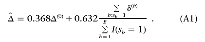
The procedure does not use bootstrap samples where no marker has P<α₁ in the final effect-size estimation, nor are they included in the denominator of the right-hand term for in equation (A1). Also, in the above effect-size estimation procedure, the top-ranked marker (if its P value is <α₁) identified in each bootstrap sample could vary from sample to sample and be different from the one based on the observed data. The main reason is that we want the bootstrap step to reflect the uncertainty in the top-ranked marker selection as it does in the observed stage I data. Sun and Bull⁷ and Ambroise and McLachlan³² provided more justifications for using this type of bootstrap step.

References

- 1.Hirschhorn JN, Lohmueller K, Byrne E, Hirschhorn K (2002) A comprehensive review of genetic association studies. Genet Med 4:45–61 [DOI] [PubMed] [Google Scholar]
- 2.Moonesinghe R, Khoury MJ, Cecile A, Janssens JW (2007) Most published research findings are false—but a little replication goes a long way. PLoS Med 4:e28 10.1371/journal.pmed.0040028 [DOI] [PMC free article] [PubMed] [Google Scholar]
- 3.NCI-NHGRI Working Group on Replication in Association Studies, Chanock SJ, Manolio T, Boehnke M, Boerwinkle E, Hunter DJ, Thomas G, Abecasis G, Altshuler D, Bailey-Wilson JE, et al (2007) Replicating genotype-phenotype associations. Nature 447:655–660 10.1038/447655a [DOI] [PubMed] [Google Scholar]
- 4.Goring H, Terwilliger JD, Blangero J (2001) Large upward bias in estimation of locus-specific effects from genomewide scan. Am J Hum Genet 69:1357–1369 [DOI] [PMC free article] [PubMed] [Google Scholar]
- 5.Allison D, Fermandez JR, Heo M, Zhu S, Etzel C, Beasley TM, Amos CI (2002) Bias in estimates of quantitative-trait-locus effect in genome scans: demonstration of the phenomenon and a method-of-moments procedure for reducing bias. Am J Hum Genet 70:575–585 [DOI] [PMC free article] [PubMed] [Google Scholar]
- 6.Siegmund D (2002) Upward bias in estimation of genetic effect. Am J Hum Genet 71:1183–1188 [DOI] [PMC free article] [PubMed] [Google Scholar]
- 7.Sun L, Bull S (2005) Reduction of selection bias in genomewide studies by resampling. Genet Epidemiol 28:352–367 10.1002/gepi.20068 [DOI] [PubMed] [Google Scholar]
- 8.Wu LY, Sun L, Bull SB (2006) Locus-specific heritability estimation via the bootstrap in linkage scans for quantitative trait loci. Hum Hered 62:84–96 10.1159/000096096 [DOI] [PubMed] [Google Scholar]
- 9.Zollner S, Pritchard J (2007) Overcoming the winner’s curse: estimating penetrance parameters from case-control data. Am J Hum Genet 80:605–615 [DOI] [PMC free article] [PubMed] [Google Scholar]
- 10.Garner C (2007) Upward bias in odds ratio estimates from genome-wide association studies. Genet Epidemiol 31:288–295 10.1002/gepi.20209 [DOI] [PubMed] [Google Scholar]
- 11.Galton F (1886) Regression towards mediocrity in hereditary stature. J Anthropol Inst 15:246–263 [Google Scholar]
- 12.Capen EC, Clapp RV, Campbell WM (1971) Competitive bidding in high-risk situations. J Petrol Technol 23:641–653 [Google Scholar]
- 13.Efron B (1983) Estimating the error rate of a prediction rule: some improvements on cross-validation. J Am Stat Assoc 78:316–331 10.2307/2288636 [DOI] [Google Scholar]
- 14.Efron B, Tibshirani RJ (1993) An introduction to the bootstrap. Chapman & Hall, New York [Google Scholar]
- 15.Bauer P, Kohne K (1994) Evaluation of experiments with adaptive interim analyses. Biometrics 50:1029–1041 10.2307/2533441 [DOI] [PubMed] [Google Scholar]
- 16.Proschan MA, Hunsberger SA (1995) Designed extension of studies based on conditional power. Biometrics 51:1315–1324 10.2307/2533262 [DOI] [PubMed] [Google Scholar]
- 17.Proschan MA, Lan KK, Wittes JT (2006) Statistical monitoring of clinical trials: a unified approach. Springer, New York [Google Scholar]
- 18.Skol AD, Scott LJ, Abecasis GR, Boehnke M (2006) Joint analysis is more efficient than replication-based analysis for two-stage genome-wide association studies. Nat Genet 38:209–213 10.1038/ng1706 [DOI] [PubMed] [Google Scholar]
- 19.Satagopan JM, Verbel DA, Venkatraman ES, Offit KE, Begg CB (2002) Two-stage designs for gene-disease association studies. Biometrics 58:163–170 10.1111/j.0006-341X.2002.00163.x [DOI] [PMC free article] [PubMed] [Google Scholar]
- 20.Satagopan, JM, Elston RC (2003) Optimal two-stage genotyping in population-based association studies. Genet Epidemiol 25:149–157 10.1002/gepi.10260 [DOI] [PMC free article] [PubMed] [Google Scholar]
- 21.Satagopan JM, Venkatraman ES, Begg CB (2004) Two-stage designs for gene-disease association studies with sample size constraints. Biometrics 60:589–597 10.1111/j.0006-341X.2004.00207.x [DOI] [PMC free article] [PubMed] [Google Scholar]
- 22.Thomas D, Xie RR, Gebregziabher M (2004) Two-Stage sampling designs for gene association studies. Genet Epidemiol 27:401–414 10.1002/gepi.20047 [DOI] [PubMed] [Google Scholar]
- 23.Scherag A, Muller HH, Dempfle A, Hebebrand J, Schafer H (2003) Data adaptive interim modification of sample sizes for candidate-gene association studies. Hum Hered 56:56–62 10.1159/000073733 [DOI] [PubMed] [Google Scholar]
- 24.Muller HH, Schafer H (2001) Adaptive group sequential design for clinical trials: combining the advantage of adaptive and of classical group sequential approaches. Biometrics 57:886–891 10.1111/j.0006-341X.2001.00886.x [DOI] [PubMed] [Google Scholar]
- 25.Spielman RS, McGinnis RE, Ewens WJ (1993) Transmission test for linkage disequilibrium: the insulin gene region and insulin-dependent diabetes mellitus (IDDM). Am J Hum Genet 52:506–512 [PMC free article] [PubMed] [Google Scholar]
- 26.Wang S, Cerhan JR, Hartge P, Davis S, Cozen W, Severson RK, Chatterjee N, Yeager M, Chanock SJ, Rothman N (2006) Common genetic variants in proinflammatory and other immunoregulatory genes and risk for non-Hodgkin lymphoma. Cancer Res 66:9771–9780 10.1158/0008-5472.CAN-06-0324 [DOI] [PubMed] [Google Scholar]
- 27.Hedges LV, Olkin I (1985) Statistical methods for meta-analysis. Academic Press, New York [Google Scholar]
- 28.Self SG, Mauritsen RH (1988) Power/sample size calculation for generalized linear models. Biometrics 44:79–86 10.2307/2531897 [DOI] [Google Scholar]
- 29.Self SG, Mauritsen RH, Ohara J (1992) Power calculation for likelihood ratio tests in generalized linear models. Biometrics 48:31–39 10.2307/2532736 [DOI] [Google Scholar]
- 30.Shieh G (2000) On the power and sample size calculations for likelihood ratio tests in generalized linear models. Biometrics 56:1192–1196 10.1111/j.0006-341X.2000.01192.x [DOI] [PubMed] [Google Scholar]
- 31.Saxena L, Alam K (1982) Estimation of the non-centrality parameter of a chi-square distribution. Ann Stat 10:1012–1016 [Google Scholar]
- 32.Ambroise C, McLachlan GJ (2002) Selection bias in gene extraction on the basis of microarray gene-expression data. Proc Natl Acad Sci 99:6562–6566 10.1073/pnas.102102699 [DOI] [PMC free article] [PubMed] [Google Scholar]
- 33.Rothman N, Skibola CF, Wang SS, Morgan G, Lan Q, Smith MT, Spinelli JJ, Willett E, De Sanjose S, Cocco P, et al (2006) Genetic variation in TNF and IL10 and risk of non-Hodgkin lymphoma: a report from the InterLymph Consortium. Lancet Oncol 7:27–38 10.1016/S1470-2045(05)70434-4 [DOI] [PubMed] [Google Scholar]
- 34.Boffetta P, Armstrong B, Linet M, Kasten C, Cozen W, Hartge P (2007) Consortia in cancer epidemiology: lessons from InterLymph. Cancer Epidemiol Biomarkers Prev 16:197–9 10.1158/1055-9965.EPI-06-0786 [DOI] [PubMed] [Google Scholar]
- 35.Proschan MA (2003) The geometry of two-stage tests. Statistica Sinica 13:163–177 [Google Scholar]
- 36.Efron B, Tibshirani R (1997) Improvement on cross-validation: the .632+ bootstrap method. J Am Stat Assoc 92:548–560 10.2307/2965703 [DOI] [Google Scholar]
- 37.Zaykin DV, Zhivotovsky LA (2005) Ranks of genuine association in whole-genome scan. Genetics 171:813–823 10.1534/genetics.105.044206 [DOI] [PMC free article] [PubMed] [Google Scholar]