Conrad: Gene prediction using conditional random fields

Abstract

We present Conrad, the first comparative gene predictor based on semi-Markov conditional random fields (SMCRFs). Unlike the best standalone gene predictors, which are based on generalized hidden Markov models (GHMMs) and trained by maximum likelihood, Conrad is discriminatively trained to maximize annotation accuracy. In addition, unlike the best annotation pipelines, which rely on heuristic and ad hoc decision rules to combine standalone gene predictors with additional information such as ESTs and protein homology, Conrad encodes all sources of information as features and treats all features equally in the training and inference algorithms. Conrad outperforms the best standalone gene predictors in cross-validation and whole chromosome testing on two fungi with vastly different gene structures. The performance improvement arises from the SMCRF’s discriminative training methods and their ability to easily incorporate diverse types of information by encoding them as feature functions. On Cryptococcus neoformans, configuring Conrad to reproduce the predictions of a two-species phylo-GHMM closely matches the performance of Twinscan. Enabling discriminative training increases performance, and adding new feature functions further increases performance, achieving a level of accuracy that is unprecedented for this organism. Similar results are obtained on Aspergillus nidulans comparing Conrad versus Fgenesh. SMCRFs are a promising framework for gene prediction because of their highly modular nature, simplifying the process of designing and testing potential indicators of gene structure. Conrad’s implementation of SMCRFs advances the state of the art in gene prediction in fungi and provides a robust platform for both current application and future research.

An accurate annotation of the protein-coding genes in an organism’s genome is essential for downstream bioinformatics analyses and the interpretation of biological experiments. The rapid increase in the rate of genome sequencing has led to increased reliance on automated annotation methods. These methods, although considerably faster, are less accurate than manual curation, as shown by the recent EGASP project on the human genome (Guigó et al. 2006; Harrow et al. 2006). More accurate automated methods are therefore critically needed.

A key problem with automated methods has been that the generative probabilistic models (generalized hidden Markov models, GHMMs) underlying the most accurate gene predictors cannot readily handle all of the diverse evidence available for gene prediction. Most of these GHMM-based gene predictors use only the genome sequence itself (Genscan, Burge and Karlin 1997; SNAP, Korf 2004; Augustus, Stanke et al. 2006; and GeneID, Parra et al. 2000) or an alignment of two or more genome sequences (Twinscan, Korf et al. 2001; N-Scan, Gross and Brent 2006; ExoniPhy, Siepel and Haussler 2004). However, human curators routinely incorporate diverse data such as EST alignments, protein homology, and comparative sequence into their decisions. This additional evidence is often difficult to model probabilistically, incorporates long-range effects, and may contain unknown dependencies with other evidence even if the model state is held constant. Each of these properties poses problems for GHMMs.

Several previous attempts have been made to improve automated gene predictions by incorporating additional evidence. The most widely adopted solution is to create an annotation pipeline that uses several different gene predictors to create preliminary gene sets that are then consolidated into a single set of predictions using the additional evidence. This consolidation involves either scripts implementing ad hoc heuristics or formalized tools such as Jigsaw (Allen et al. 2004; Allen and Salzberg 2005), ExonHunter (Brejová et al. 2005), or Glean (Elsik et al. 2007).

Applying an annotation pipeline to a new organism is generally a complex and labor-intensive process since each of the tools in the pipeline will typically require some form of organism-specific training, which often requires assistance from the original author of the tool. Instead of combining several complex tools using heuristics, it would be preferable to have a single gene prediction tool that is easily retrained for new genomes, incorporates any available data, and provides the highest available accuracy given those data. Several theoretical extensions to GHMMs have been proposed to handle this, including handcrafted heuristics for particular feature types (Yeh et al. 2001), a mixture-of-experts approach applied at each nucleotide position (Brejová et al. 2005), and decision trees (Allen et al. 2004; Allen and Salzberg 2005). However, none of these extensions addresses all of the problems above in a general way.

In this paper, we address these problems by applying the theoretical framework of conditional random fields (CRFs) (Lafferty et al. 2001) to the problem of gene prediction. Unlike GHMMs, CRFs are capable of incorporating evidence that contains long-range effects and unknown dependencies without requiring any probabilistic modeling of the observation data. A specific CRF variant called semi-Markov conditional random fields (SMCRFs) (Sarawagi and Cohen 2005; Vinson et al. 2006) can exactly reproduce the predictions of a GHMM but is strictly more expressive: The generative features inherited from GHMMs can be combined with discriminative features representing new evidence, and all features regardless of origin are treated equally by the SMCRF framework.

SMCRFs can not only incorporate new evidence more easily than a GHMM, but might also be able to make more accurate predictions from the same information. SMCRFs are an example of discriminative modeling, in which one directly models the conditional probability Pr(Y|X) of hidden states given observations, while GHMMs are an example of generative modeling, in which one models the joint probability Pr(Y,X) of hidden states and observations (Ng and Jordan 2001). Although GHMMs have been the dominant approach to gene prediction since 1997 (Burge and Karlin 1997), discriminative modeling has also been attempted. The gene predictor GAZE (Howe et al. 2002) uses the same concepts as CRFs but is based on a much earlier theoretical framework of conditional maximum likelihood (Stormo and Haussler 1994). Culotta et al. (2005) performed a proof-of-concept study using standard CRFs, and Gross et al. (2006) presented a training algorithm to maximize an approximation of the nucleotide accuracy of the posterior decoding.

The gene predictor CRAIG (Bernal et al. 2007) used SMCRFs and demonstrated improvements over single-genome gene predictors using several benchmark data sets, but did not use comparative information and was not more accurate than the best comparative gene predictors. CRAIG is trained using an online large-margin algorithm and uses feature sets developed from scratch. Our approach, Conrad, differs from CRAIG in three important respects. First, Conrad uses genome comparisons and, as shown below, actually improves upon the state of the art for the species studied. Second, Conrad uses features inherited from GHMMs as a starting point, building on existing research and enabling direct comparisons of generative versus discriminative approaches. Third, we introduce a novel training method called maximum expected accuracy (MEA), which allows us to optimize a measure of accuracy specific to gene prediction.

We implement the SMCRF framework with the conditional maximum likelihood (CML) and MEA training algorithms in the gene predictor Conrad. An earlier version of Conrad lacking the MEA training and semi-Markov capability was presented in Vinson et al. (2006). Conrad’s implementation applies machine learning and software engineering principles toward the goal of creating a single, easily trained gene predictor accurate enough to replace existing complex annotation pipelines. Conrad can be used to predict protein-coding genes using a genome sequence or an alignment of related species, but is configurable and allows full control over the data and features in the model and the algorithms for training and inference. It can thus be extended to incorporate additional data and used as a platform for further research in gene prediction or the application of SMCRFs to other problems. Conrad is written entirely in Java and is freely available under the GPL open-source license.

We tested Conrad on two fungal genomes, and on each it outperformed the most accurate available gene predictor. On the human pathogen Cryptococcus neoformans Conrad outperforms Twinscan, previously the most accurate gene predictor trained for C. neoformans. On Aspergillus nidulans, Conrad outperforms Fgenesh, the gene predictor used in the reference GenBank annotation. Using controlled experiments we demonstrate how these performance improvements result from the theoretical advantages of SMCRFs. We first show that for gene prediction the discriminative training methods of SMCRFs outperform the generative methods of GHMMs and then demonstrate that the SMCRF’s ability to incorporate additional data enables a further enhancement in accuracy.

Methods

Conrad is implemented using the theoretical framework of conditional random fields. CRFs express the conditional probability Pr(Y|X) of a set of hidden states Y given observation X (Sutton and McCallum 2006). A CRF assigns a probability to the hidden states Y by normalizing a weighted exponential sum of feature sums F_j:

where w_j denotes the weight for feature sum F_j, and Z_w(X) is the normalizing constant. For gene prediction, we assume that the hidden states Y are linearly structured as a vector of labels y₁,y₂,y₃. · · ·, y_n, with one label such as “exon” or “intron” per nucleotide of the sequence to be annotated. Equivalently, Y can be represented as a segmentation of the nucleotide sequence into a variable number p of intervals (t_i,u_i,v_i)^_i=1p with starts t_i, stops u_i, and labels v_i:

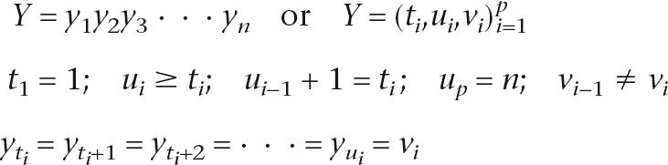and where restrictions on the allowed transitions v_i−1 → v_i ensure that all gene structures are plausible. For example, the transition from “intergenic” to “exon” can only occur at an ATG start codon (see Supplemental material). In this paper, we use both the label y₁,y₂,y₃, · · ·, y_n and interval (t_i,u_i,v_i)^_i=1prepresentations for Y as appropriate. Equations involving only X and Y are general statements that do not depend on the linear chain structure and also apply to CRFs on arbitrary graphical models.

As with gene predictors based on GHMMs, we impose the constraint that each interval (t_i,u_i,v_i) interacts only with its immediate neighbors. Thus, the feature sum F_j can be written as a sum of localized feature functions f_j,

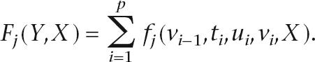This type of CRF is called a semi-Markov CRF (SMCRF) (Sarawagi and Cohen 2005). To use an SMCRF to annotate a genome sequence given observations X, one computes the segmentation Y with the highest conditional probability Pr(Y|X). The “inference algorithms” to compute this are essentially the same as those used in GHMMs (see Supplemental material).

The key issues in the application of SMCRFs to gene prediction are the design of the feature functions f_j and the selection of the weights w_j. Feature functions use the observations X to assign a real value to each labeling of each possible interval and capture properties of the observation data relevant for classification. They are not required to be independent or have a probabilistic interpretation. It is straightforward to use GHMM models as a source of feature functions (which we call “generative features,” see below), and we use a state of the art phylo-GHMM to provide the core feature set for Conrad. By using this approach, we enable Conrad to behave as either a GHMM or an SMCRF. We further define a handful of “discriminative features” to capture information from phylogenetic footprinting, insertion/deletion events in multiple alignments, and EST alignments.

To select the weights for a CRF, one provides example annotations and uses a training algorithm to select weights that, according to some criterion, perform best on the training data. We discuss two training algorithms: CML, which is the algorithm used most often with CRFs, and MEA, which we developed to maximize accuracy measures that are specific to gene prediction.

Semi-Markov CRF equivalent of a phylogenetic GHMM

Currently, the best available predictors utilize a phylogenetic GHMM with explicit state durations, which we will refer to as a phylo-GHMM (Pedersen and Hein 2003; McAuliffe et al. 2004; Siepel and Haussler 2004; Brown et al. 2005). We use this model as the starting point for SMCRF development.

A GHMM is a model of the “joint probability” Pr(Y,X) of a and the observations X:

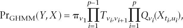where π are the initial probabilities, T is the transition matrix, and Q₁,Q₂, · · ·, Q_M are the emission models, where Q_v(X_t,u) is the probability (including length distribution) of hidden state v emitting the observed sequence X from t to u. The “conditional probability” can be obtained by normalizing Pr_GHMM(Y|X) = Pr_GHMM(Y,X)/Pr_GHMM(X), and it is the conditional probabilities of a GHMM that are ultimately used for gene prediction.

The conditional probabilities of a GHMM are mathematically equivalent to an SMCRF using a single feature f_GHMM with weight 1.0:

Instead of representing the entire GHMM with a single SMCRF feature, we split the components of f_GHMM into a collection of simpler features, each with weight 1.0. We call the features designed in this way “generative features” and split a phylo-GHMM into the following 22 generative features (see Supplemental material for more information on the features):

The five reference features model the nucleotide composition of the reference sequence. Each feature outputs the log probability of the current nucleotide based on a third-order Markov model learned from the training data for a subset of the states. The features do not include probabilities for nucleotides at the edges of states, which are covered by the boundary features.

The three length features compute the log probability for state length distributions of introns, exons, and intergenic regions. Intergenic distances are modeled using an exponential distribution, and the exon and intron distributions are modeled as a mixture of two gamma distributions.

The transition feature models the frequency of various state transitions and corresponds to the transition matrix of a GHMM. The only parameter fit from the training data for this feature is the average number of exons per gene. All other parameters are set to make the model symmetric so that genes on either strand or in any frame are preferred equally.

The eight boundary features model nucleotide signals that occur at state boundaries. These signals include splice donor and acceptor signals and start and stop codons. Each of the eight features returns the log probability of a PWM learned from the training data for a specific boundary.

The five phylogenetic features incorporate data from multiple species, one feature each for intergenic regions, introns, and the three reading frames. Each feature returns the log probability of a column in the multiple alignment (based on probabilistic models of nucleotide evolution) conditioned on the nucleotide in the reference sequence.

The SMCRF model using only the reference, length, transition, and boundary features with weights fixed at 1.0 is called ConradG-1. ConradG-1 exactly reproduces the conditional probabilities of a GHMM and is comparable to single-genome gene predictors such as Genscan (Burge and Karlin 1997), GeneID (Parra et al. 2000), or Fgenesh (Salamov and Solovyev 2000).

The SMCRF models using all the generative features defined above with weights fixed at 1.0 are called ConradG-2, ConradG-3, etc, depending on the total number of species used by the phylogenetic feature. These models exactly reproduce the conditional probabilities of a phylo-GHMM, and ConradG-2 is comparable to the two-genome gene predictor Twinscan. Table 1 summarizes these models and the other models referenced in this paper.

Table 1.

Definition of the various Conrad models

The first character indicates the training method and subsequent characters indicate the presence of various discriminative features. The final number indicates the number of species used, including the reference. The type of model is either SMCRF or GHMM. The training method is either CML or MEA for SMCRFs.

Training the weights using conditional maximum likelihood (CML)

The traditional way of training the weights w_j of a CRF is CML. Assuming a single training sequence of training data (Y⁰,X⁰), this is:

The function log(Pr_w(Y⁰|X⁰)) is a concave function of w, because its Hessian is the negative of the covariance matrix of the random variables F_j(Y,X⁰) when Y is drawn from Pr_w(Y|X⁰). Thus, log(Pr_w(Y⁰|X⁰)) is guaranteed to have a single local maximum w_CML, which is also the global maximum.

In practice, one maximizes log(Pr_w(Y⁰|X⁰)) using a gradient-based function optimizer (Zhu et al. 1994; Wallach 2003), and the algorithms for computing the gradient depend on the specific variant of CRF. For SMCRFs, computing the gradient involves dynamic programming to perform a forward and backward pass through the training data. The computation time is linear in both the length of training data and the length of the longest allowed interval (see Supplemental material).

We define the models ConradC-n (n ≥ 1) to have the same features as ConradG-n (reference, length, transition, boundary, and phylogenetic features), but with weights trained by CML (see Table 1 for the full list of models).

Training the weights using maximum expected accuracy (MEA)

To evaluate gene predictions one measures the accuracy of the inferred segmentation. Conditional maximum likelihood indirectly optimizes accuracy by maximizing the likelihood of the correct segmentation as provided in the training examples. In principle, we expect that directly optimizing the accuracy of the inferred segmentation would improve performance. However, this is intractable to optimize because altering the weights causes different segmentations to be inferred, which result in discontinuous changes in accuracy. To avoid this complication, we optimize the weights using an objective function defined as the expected value of the accuracy over the entire distribution of segmentations defined by the SMCRF. We call this training approach maximum expected accuracy (MEA).

Given training data (Y⁰,X⁰), one can define the accuracy of a path Y = y₁y₂y₃· · ·y_n to be the similarity between Y and Y⁰ given X⁰. Similarity can be defined using metrics relevant for a given application, and we consider similarity functions S that can be evaluated as a sum of dinucleotide comparisons between the hidden paths:

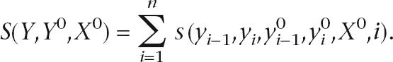Given S, we define the objective function A as the expected value of S, and select weights to maximize A:

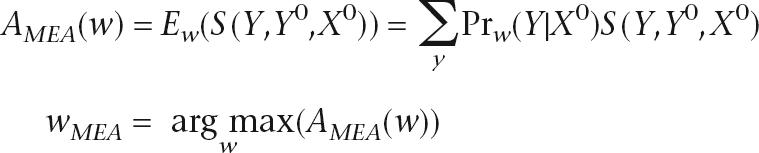We can efficiently compute gradients of the objective function A_MEA(w) (see Supplemental material) and use a gradient-based function optimizer to find a local maximum. Since the objective function A_MEA(w) is not a concave function of w and we are not guaranteed to find the global maximum, we set the initial weights using the results of CML training.

For our application to gene prediction, we define the similarity function S_NUCLEOTIDE to be the number of nucleotides at which the hidden state is correct, and S_SPLICE to be the number of nucleotides called correctly plus 200 times the number of splices called correctly. We define the SMCRF models ConradN-n and ConradS-n to have the same features as ConradG-n, with weights trained by MEA with similarity functions S_NUCLEOTIDE and S_SPLICE, respectively (see Table 1 for the full list of models).

Still other training methods have been proposed for CRFs. One approach is to maximize the accuracy of the posterior decoding (Gross et al. 2006) by approximating the step function by a steep sigmoid and using gradient descent. Margin-based methods for training CRFs in another context have been used in Taskar et al. (2003), and for training SMCRFs for gene prediction in Bernal et al. (2007).

Discriminative features

Discriminative features are those feature functions that do not have a probabilistic interpretation. The ability of SMCRFs to incorporate discriminative features is what enables them to incorporate evidence that contains long range effects or unknown dependencies, or is simply difficult to model probabilistically. The SMCRF training algorithms described above (except for the GHMM “training method” of fixing the weights at 1.0) will assign optimal feature weights to any real valued feature functions, not just those that correspond to valid probability models. This is the key distinction that allows SMCRFs to take advantage of diverse evidence for gene prediction that has not been possible to incorporate into phylo-GHMMs.

We designed two groups of discriminative features to represent information that is routinely used by manual curators to refine gene predictions but has so far been difficult to incorporate in phylo-GHMM-based gene predictors, and one group of features as a positive control that has been successfully implemented in GHMMs. These discriminative features are all 0–1 indicator functions, but this is purely for convenience and is not a requirement of either the SMCRF framework or our implementation in Conrad.

The six gap features capture information from the pattern of gaps in a multiple alignment that is not captured by the phylogenetic features or by phylo-GHMMs:

Gaps in a multiple alignment are indicative of insertions or deletions (indels) in the evolutionary history of one of the aligned species, and occur rarely in functionally conserved regions of a genome such as exons. In particular, those indels that are not a multiple of three disrupt the translation of a protein and almost never occur in exons (Kellis et al. 2003). The most systematic attempts at incorporating multiple alignment gaps in a phylo-GHMM have been the one made by Siepel and Haussler (2004), which only represents the case of phylogenetically simple, nonoverlapping gaps, and Gross and Brent (2006), which only has sufficient data to train a first- or second-order model of the columns in a multiple alignment and thus cannot exploit the crucial mod-3 length of gaps.

The three footprint features per species indicate the positions at which each species is aligned:

Coding sequences are more likely to be aligned than noncoding regions for two reasons. First, they are less likely to have been deleted in the evolution of the informant species. Second, the coding regions tend to be more conserved and therefore easier to align than noncoding sequences, although this also depends on the method of sequence alignment. These effects are not captured in phylo-GHMMs. One approach is to treat the absence of an informant species in the alignment as missing information (Siepel and Haussler 2004). Another is to extend the alphabet of four nucleotides to include “gap” or “unaligned” as in Gross and Brent (2006), but this approach requires manually tuning a “conservation score coefficient” (usually between 0.3 and 0.6) to achieve the best predictive performance. SMCRF footprint features require no manual tuning, because the proper weights are set automatically during training.

The difficulty of incorporating diverse information in a GHMM comes not from incorporating any one type of information, but in combining many types of information within the same model. For example, Twinscan captures information similar to the gap and footprint features by extending a single genome GHMM with a conservation track modeled with a high-order Markov model. However, this approach does not generalize naturally to multiple phylogenetically related species and lacks the realism of evolutionary models of nucleotide substitution. Conversely, phylo-GHMMs such as N-Scan or ExoniPhy exploit phylogenetic relationships and evolutionary models of nucleotide substitution but, as described above, fail to fully capture the gap and footprint features. A second example is hexamer composition and CpG frequency: The former is indicative of the state of a stretch of nucleotides, the latter is indicative of a nearby translation start site, but the two are intimately related and difficult to combine in the same GHMM. In contrast, a CRF provides a consistent mechanism that allows any available feature functions to be combined in a model and trained appropriately.

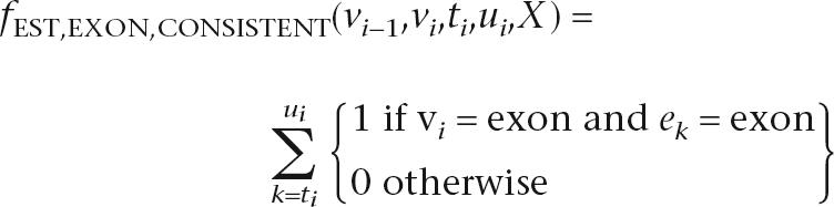
The nine EST features relate the alignment of ESTs to the states and transitions of the hidden sequence, and resemble those in Wei and Brent (2006). ESTs are experimentally determined sequences of randomly sampled mRNA and provide strong evidence for the transcription of a sequence. However, ESTs are usually partial and also contain the untranslated regions bounding each coding sequence. The nine EST features capture information about individual base and splice junction agreement with ESTs and account for the fact that multiple EST alignments at a given position will often disagree. The exon and splice acceptor indicator features are defined as follows:

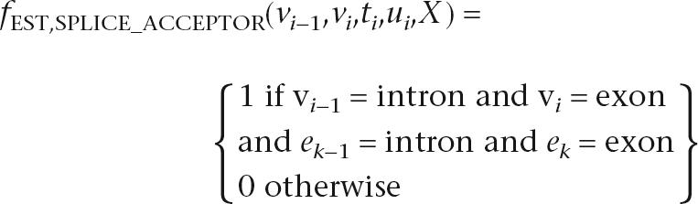where e_k is an additional observation indicating the EST evidence available at each position. The other seven features are defined similarly (see the Supplemental material for full details on the EST features).

We name SMCRF models containing discriminative features by appending a letter to the end of the model name for each feature, using F, G, and E for footprint, gap, and EST features, respectively (see Table 1 for the full list of models). Discriminative features can only be used with the SMCRF models (those trained with CML or MEA) and not the GHMM models (those with weights fixed at 1.0).

Conrad training

We implemented the theoretical framework described above in the gene predictor Conrad. To train each SMCRF model one supplies a model parameter file (a list of features and a training method) and a set of training data (which includes both hidden sequences and observations). Conrad first uses the training data to learn numerical parameters for the features, such as the intron length distribution, the position weight matrix for the splice sites, and the rates of nucleotide sequence evolution. Conrad then trains the feature weights (if CML or MEA is specified) or sets the feature weights to 1.0 (to reproduce a GHMM), and saves the learned feature parameters and feature weights as a trained SMCRF model, which can be used to make predictions on new input data. To evaluate the trained SMCRF models, we generated Conrad predictions on a testing set and measured the accuracy of the predictions. Detailed instructions for running Conrad are available at the Conrad Web site (http://www.broad.mit.edu/annotation/conrad).

Experimental design

For our cross-validation experiments, we created a reference set of high-confidence genes in each organism by selecting genes from the GenBank annotation that had full EST support along their entire length and an open reading frame of at least 100 bases. For C. neoformans, we additionally required that each gene have at least two exons. Each reference gene, along with 200 bases of padding on each side, was treated as a separate sequence. For each desired training set size, we created 10 random train-test partitions of this reference set. We then performed specific comparisons using this cross-validation framework. For each model, we measured sensitivity and specificity at the nucleotide, exon, and gene levels as described in Burset and Guigó (1996) for each of the partitions (see Supplemental material for full details on the training and testing sets).

C. neoformans has a 19 Mb genome containing ∼7000 genes with complex gene structures averaging six exons per gene. It is an ideal test case due to deep EST sequencing of strain JEC21 (Loftus et al. 2005) and the availability of genomes for four closely related strains (var. grubii H99, var. gatti R265, var. gatti WM276, var. neoformans B-3501A), which we aligned using MULTIZ and TBA (Blanchette et al. 2004). Our total reference set size was 1105 genes. To evaluate the effects of training sets size, we created partitions with training sets sizes of 50, 100, 200, 400, 600, 800, and 1000 genes. To evaluate the effectiveness of different weight training methods, we compared models with the same feature sets. To evaluate the effects of feature selection, we held the training method constant and compared the models using different combinations of features. Because ESTs were used in the construction of the reference set of genes, the EST feature served as a positive control: We had a strong expectation that the EST feature should lead to improved performance on the reference gene set (Wei and Brent 2006). We also measured the effect of training set size on testing accuracy and the size of the generalization gap (the difference between performance on the training and testing sets).

A. nidulans has a 30 Mb genome with >10,000 genes. We divided the reference set of 574 genes into 10 random partitions with 300 training genes and 274 test genes. We then examined the effects of several different choices of informant species among nine fully sequenced genomes from the Aspergillus clade.

To benchmark Conrad against other gene predictors, we performed chromosome/genome testing on both organisms. The reference gene sets are highly accurate and useful for cross-validation, but any meaningful comparison of gene callers must be done using full chromosomes and evaluated against a data set not biased toward any particular gene predictor. We compared Conrad to the two most accurate gene predictors that have been trained for C. neoformans (Twinscan and GeneID) by running each on chromosome 9 and comparing results against all available EST data. Conrad was trained on the set of 1048 reference genes not on chromosome 9. GeneID was retrained using the full set of trusted genes by R. Guigó and F. Camara (pers. comm.) and an updated version of Twinscan was run for us on chromosome 9 by M. Brent and R. Brown (pers. comm.). On A. nidulans, we compared Conrad to Fgenesh on the entire genome, once again comparing results against all available EST data. Conrad was trained on the entire reference set and Fgenesh was trained by Softberry (Salamov and Solovyev 2000).

Results

Semi-Markov CRF training approaches

Our cross-validation experiments on C. neoformans demonstrate the relative performance of Conrad models using various feature sets, training methods, and training set sizes. The results of these experiments are presented in Figure 1. For each model, Figure 1 shows the gene sensitivity (percentage of reference genes completely correct in the testing set) across different training set sizes and the full set of testing accuracy statistics for models trained on the 600-gene training sets. The models are grouped according to the data they use for prediction. Those models that use all available input data perform the best, followed by the two-species predictors using various training methods and then the single-species predictor.

Figure 1.

Performance of Conrad models in the C. neoformans cross-validation tests. The graph on the left shows average gene sensitivity (percentage of reference genes completely correct in the testing set) across 10 replicates based on model and training set size. Solid lines are performance on the test set, and dotted lines are performance on the training set (not all training sets are shown). The bars represent standard deviation across the replicates. The table on the right shows the full set of testing accuracy statistics for the models on the 600-gene training sets.

The middle group of models in Figure 1 all use the same two-species alignments and feature set but differ in their training methods, enabling a direct comparison of GHMM (generative) versus SMCRF (discriminative) training approaches. The three discriminative training methods outperform generative training on all metrics except nucleotide sensitivity where all methods achieve similar performance. At the gene level, the discriminative approaches are on average 8.4% more sensitive (61.1% compared to 52.7%) and 6.9% more specific (61.2% compared to 54.1%) than generative training. For exons, discriminative training improves sensitivity by 3.5% (85.8% versus 82.3%) and specificity by 3% (90% vs. 87%).

The performance of the different discriminative training methods was essentially equivalent. Conditional maximum likelihood training (ConradC-2) had gene sensitivity and specificity averaging 61.3% and 61.8% with standard deviations of 2.6% and 2.8%, respectively. The other methods had specificities within 0.5% (61.1% for ConradN-2 and 60.8% for ConradS-2) and sensitivities within 1.0% (61.0% for ConradN-2 and 60.8% for ConradS-2). Exon and nucleotide statistics for these models were also within a percentage point. The discriminative training methods showed similar performance even on more complicated models incorporating additional species and features, and so only the results for the “S” models (MEA with splice bonus) are presented for those models.

The performance of all of the training methods has a consistent profile as the number of genes in the training set changes. Consistent with previous findings (Allen and Salzberg 2005), training methods reach full accuracy at ∼600–800 genes and suffer only a nominal reduction in accuracy using just 200–400 genes. The dotted lines in Figure 1 show the performance of the ConradC-2 and ConradSFG-5 models on their training set, and other models are similar. The difference between performance on the training set and the testing set is known as the “generalization gap.” We can see that it closes significantly for most models by 400 genes and disappears completely with 600 genes. The apparent drop in accuracy at 1000 genes likely results from increased variability due to the small size of the test set (105) for these trials.

The discriminative training methods are significantly more computationally expensive than the generative methods due to the numerical optimization required. Our tests were run on the Broad Institute compute farm, which consists of 200 Linux servers, each with two x86 processors between 2.5 and 3.2 GHz and 4–8 GB of memory. The GHMM took an average of 39 CPU-seconds per megabase for training, while CML averaged 6–8 CPU-hours and MEA averaged 8–12 CPU-hours per megabase depending on the number of features used. Even with this roughly 1000-fold difference, complex discriminative models can be trained on realistic small genome data sets in a day or two on a standard PC. The extra cost is incurred only during training, since the inference algorithms for all approaches are identical, taking an average of 8.5 min/Mb.

Improved accuracy with discriminative features

The models in Figure 1 demonstrate the effects of feature selection. Increasing the number of species from one to two to five improves gene sensitivity by 11.3%, from 53.3% to 60.8% to 64.6%. Incorporating the gap and footprint features, which use the same input data as the generative phylogenetic models, further improves sensitivity of the five species model by 5.5% to 70.1%.

By incorporating EST features into the model, we obtain significant performance improvements. The ConradSFGE-5 model achieves gene sensitivity of 86.0%, a 15.9% improvement over not having EST data. This model was trained using only half of the EST data (EST data was removed from half of the genes), to avoid overtraining effects, and tested using all EST data. We also trained the model using the full complement of EST data, which performed slightly better on the cross-validation set but did not generalize as well during the whole chromosome testing (data not shown).

Comparison with Twinscan and GeneID

We compared Conrad to GeneID (Blanco et al. 2003) and Twinscan by training on isolated genes and predicting on a full chromosome sequence, simulating a typical production annotation. The results are presented in Table 2, which shows that Conrad outperforms existing gene predictors using the same data and is also capable of incorporating additional data to further improve performance.

Table 2.

Performance of Conrad and other gene callers on C. neoformans chromosome 9

The models are grouped by the evidence they used as input: single gene sequence, pairwise alignment, and then all available data. Predictions were compared to available EST (expressed sequence tag) evidence using a custom set of metrics designed to handle partial information from ESTs. Shown are the total number of genes and exons predicted by each model and the number of those predictions that overlapped EST evidence. Of those predictions overlapping EST evidence, the percent where the EST and gene predictions agree is shown. Also included is the total number of EST clusters that did not overlap any prediction, indicating probable missed genes.

The ConradSFG-2 model uses the same input data as Twinscan, and outperformed it by 12.9%, with 78.4% gene sensitivity, compared to 65.5% for Twinscan. Examining the various two-species models allows us to dissect this performance improvement. The ConradG-2 model implements a two-species phylo-GHMM theoretically similar to Twinscan and achieves nearly identical performance of 65.7%, supporting the hypothesis that the performance improvements seen in other Conrad models are the result of the theoretical advances and not simply implementation differences.

Using discriminative training improves performance. The ConradS-2 model differs from ConradG-2 only in its training method and achieves 5.4% better performance. Although the cross-validation experiments showed very small differences between the various discriminative training methods, on the full chromosome test we see a 4.2% difference between the various discriminative methods, with MEA with the splice bonus outperforming MEA using nucleotide accuracy, which in turn outperforms conditional maximum likelihood. Since this was a single experiment, we do not have a measure of the variability of these estimates.

The selection of features in the model also affects performance. The ConradSFG-2 model adds the gap and footprint features to the ConradS-2 model and obtains a 7.3% gain in performance. Moving from two species to five species, the ConradSFG-5 model provided a 4.0% improvement to 82.4%. The single-species model, ConradS-1, achieved 63.3% accuracy: 22.5% better than GeneID and only 2.2% below Twinscan.

As expected, the EST features provide a large gain and improve accuracy a further 12.1% to 94.5%. However, ConradSFGE-5 model differs from the other models in the number of genes called and the average length of each gene. These differences may be a consequence of the training set not having the same distribution of EST evidence as chromosome 9. Because the reference genes all had full EST support, we randomly selected one half of the training genes and removed all of their EST evidence as a way of simulating a more realistic distribution. The accuracy improvement indicates this is a reasonable approach. However, there are still notable differences between our training set and chromosome 9, such as the lack of genes with partial EST support.

Application to A. nidulans

The Aspergillus clade has nine fully sequenced genomes, allowing us to compare the effects of different choices of informant species on gene prediction accuracy. The results of cross-validation experiments using a 300-gene test set and 274-gene training set are shown in Figure 2.

Figure 2.

Accuracy results for the ConradSGF-n model on A. nidulans using several different combinations of informant species. Branch lengths are in substitutions per site based on a set of highly conserved housekeeping genes.

The single-species model using only A. nidulans has gene sensitivity, 65.2%, and all of the comparative models outperform the single-species predictor. The two species models using A. oryzae and A. fumigatus models perform ∼9% better than the single-species model. However, the two species C. immitis model only outperforms the single-species model by 3.4%, which may indicate that the branch length between this outgroup species and reference genome is too large to be useful. Adding additional species beyond two increases the accuracy further, but the gains appear to be more modest (74.1% to 76.5% gene sensitivity).

We compared Conrad to Fgenesh, the gene caller used for the GenBank annotation of A. nidulans. We ran both predictors on the full genome and compared the results against the available ESTs. We used the single-species model ConradS-1 to get a fair comparison against Fgenesh, which is also a single-species predictor. Both programs predicted similar numbers of exons (37,263 for Fgenesh and 37,084 for Conrad), but Conrad generally predicted more, shorter genes than Fgenesh (13,620 genes averaging 1040 bases versus 10,146 genes averaging 1544 bases). Conrad was more specific than Fgenesh, with 67.6% of genes overlapping ESTs having agreement compared to 64.8%. Fgenesh was 0.6% more specific than Conrad at exon predictions (76.0% vs. 76.6%), while Conrad was 3.0% more specific than Fgenesh at intron predictions (78.9% vs. 75.9%).

Understanding the trained models

Examining the weights of a trained model can provide some insight into the relative importance of the features used for classification. If all features are similarly scaled, as is the case when a model contains only generative features, larger weights indicate more important features. This illustrates a benefit of discriminative training (SMCRFs), which allows more useful features to be given higher weights, as compared to generative training (GHMMs) where all weights are fixed at 1.0.

Figure 3 shows the weights selected by MEA algorithm for the ConradS-2 model for both A. nidulans and C. neoformans, averaged across the 10 replicates. Encouragingly, when the same feature is repeated across reading frames (donor and acceptor) or strand (phylogenetic exon and intron), the weights are very similar. Some differences were unexpected, such as the weights for donor PWMs being twice as large as those for acceptor PWMs. This suggests that donor PWMs are more useful than acceptor PWMs for classification in these organisms.

Figure 3.

Average weights for the ConradS-2 model on both the Cryptococcus 600-gene training sets and the Aspergillus training sets. Bars show the standard deviation across 10 replicates.

The length features have the largest variation across states. The intron length feature has a very strong weight in C. neoformans, which is consistent with previous investigations showing intron lengths to be important signals for this organism (Tenney et al. 2004) and confirming the need for the extension of CRFs to SMCRFs in Conrad to handle explicit length distributions. This weight is lower in A. nidulans where intron length is less important. The intergenic length feature has a large negative weight, which is probably an artifact of our training method, which pads all training genes with 200 bases of intergenic sequence.

Discussion

The implementation of semi-Markov conditional random fields (SMCRFs) in Conrad advances the state of the art in gene annotation in fungi and provides a robust platform for both current application and future research. The first advance comes from the use of discriminative versus generative training. Using the same set of generative features, we consistently achieve greater accuracy using an SMCRF with feature weights set by conditional maximum likelihood (CML) or maximum expected accuracy (MEA) than using a generalized hidden Markov model (GHMM) with feature weights fixed at 1.0. The second advance is the ease of incorporating additional information and the resulting improvement in accuracy. For example, the gap and footprint features increase accuracy by extracting unused information from the multiple alignments; the use of more informant species increases accuracy; and the use of EST data further increases accuracy. Importantly, all of these different features can be easily combined together in a single model. SMCRF features do not have to be probabilistic models and can contain long-range effects or unknown dependencies with other features. Conrad achieves a level of accuracy greater than existing methods for both C. neoformans and A. nidulans, two fungal genomes with highly dissimilar gene structures.

Conrad is a robust platform. In addition to the thousands of training and testing cycles done in our cross-validation experiments, it has been incorporated into the Broad Institute’s annotation pipeline for eukaryotic genomes and is currently being used on Phytophthora infestans, Fusarium oxysporum, and Culex pipiens quinquefasciatus. Conrad is freely available under a GPL open-source license and is highly customizable. A user can retrain Conrad for another species, reconfigure Conrad to use a different combination of features and training method, write entirely new features, or define a new measure of gene accuracy for the MEA algorithm.

Designing improved feature sets is one avenue for further improvements in gene prediction accuracy. In this paper, we began the development of Conrad with a core set of features inherited from phylo-GHMMs. Thus, we started with a state-of-the-art model and observed the benefits of discriminative training by directly comparing the GHMM and SMCRF models. This approach of seeding discriminative models with features derived from generative models has been used in other fields (Ulusoy and Bishop 2005). In some cases, the generative features were eventually replaced with purely discriminative features that provide higher accuracy, and this may be a reasonable approach for gene prediction, as in Bernal et al. (2007).

We are currently pursuing a handful of technical improvements to further improve accuracy and extend Conrad to mammalian genomes. First, the current model caps the length of each interval (which is appropriate for fungi), but for application to mammalian genomes, we are implementing a state transition model that supports arbitrarily long introns and intergenic regions. Second, we are developing state models that include UTRs because this is useful for some downstream applications and because it may lead to improved accuracy (Brown et al. 2005). Finally, we are creating a parallel version that can utilize a compute cluster to rapidly train on large data sets.

Although not pursued in this paper, one can incorporate long-range biological interactions in a SMCRF by writing feature functions that depend on the entire set of observations. For example, the presence of upstream CpG islands is often associated with gene promoters, and one could capture this effect with a feature that is 1 at the start of transcription if there is a CpG island within 2 kb upstream, and 0 otherwise. This type of interaction is impossible to incorporate in a GHMM without significantly altering the model and increasing the number of states. Other long-range signals that may be useful for gene prediction are exonic splicing enhancers, chromatin methylation patterns, transcription assays using genomic tiling arrays, and DNase hypersensitive sites.

As features are added to include more information, it becomes increasingly important to ensure that the training set is representative of the test set. For example, using the EST features and all of the EST data on the C. neoformans reference set led to a model that performed very well in cross-validation but poorly on an entire chromosome. We addressed this problem by randomly deleting half the EST evidence in the training set. This improved performance in the whole chromosome test significantly, but the elevated number of short genes suggests that some bias still exists. Since most training sets today contain only positive examples, this issue will be especially relevant for features that provide negative evidence, such as repeat regions or known RNA genes that indicate a given region of sequence is likely not a protein-coding gene.

SMCRF training algorithms are another avenue for improvement. In terms of accuracy, we might already be in the realm of diminishing marginal gains: Holding the feature set constant, the models trained discriminatively all had prediction accuracies greater than the corresponding GHMM but indistinguishable from each other (with the possible exception of MEA-splice having better performance on a full chromosome of C. neoformans). However, using a customizable definition of accuracy, as in MEA, may be useful in reducing the impact of low-confidence data or including alternate splice forms in the training data, perhaps by considering several variants equally acceptable during training. Additionally, entirely different training approaches can be used, including Maximum Parse Accuracy (Gross et al. 2006) and margin-based approaches (Taskar et al. 2003; Raetsch and Sonnenburg 2006; Bernal et al. 2007).

Conrad shows that the theoretical advantages of SMCRFs over GHMMs translate into improved performance and more flexible models, removing fundamental obstacles that have led to the persistent gap between the performance of automated and manual annotation methods. Conrad’s initial results presented here already outperform the best available gene predictors on two very diverse fungal genomes. However, we believe the most significant contribution of this work is the potential it creates for future improvements in gene prediction. Conrad provides a solid theoretical framework with a robust open-source implementation that allows any researcher to add new data and features to improve an already state-of-the-art automated gene caller.

References

- Allen J.E., Salzberg S.L., Salzberg S.L. JIGSAW: Integration of multiple sources of evidence for gene prediction. Bioinformatics. 2005;21:3596–3603. doi: 10.1093/bioinformatics/bti609. [DOI] [PubMed] [Google Scholar]
- Allen J.E., Pertea M., Salzberg S.L., Pertea M., Salzberg S.L., Salzberg S.L. Computational gene prediction using multiple sources of evidence. Genome Res. 2004;14:142–148. doi: 10.1101/gr.1562804. [DOI] [PMC free article] [PubMed] [Google Scholar]
- Bernal A., Crammer K., Hatzigeorgiou A., Pereira F., Crammer K., Hatzigeorgiou A., Pereira F., Hatzigeorgiou A., Pereira F., Pereira F. Global discriminative learning for higher-accuracy computational gene prediction. PLoS Comput. Biol. 2007;3:e54. doi: 10.1371/journal.pcbi.0030054. [DOI] [PMC free article] [PubMed] [Google Scholar]
- Blanchette M., Kent W.J., Riemer C., Elnitski L., Smit A.F.A., Roskin K.M., Baertsch R., Rosenbloom K., Clawson H., Green E.D., Kent W.J., Riemer C., Elnitski L., Smit A.F.A., Roskin K.M., Baertsch R., Rosenbloom K., Clawson H., Green E.D., Riemer C., Elnitski L., Smit A.F.A., Roskin K.M., Baertsch R., Rosenbloom K., Clawson H., Green E.D., Elnitski L., Smit A.F.A., Roskin K.M., Baertsch R., Rosenbloom K., Clawson H., Green E.D., Smit A.F.A., Roskin K.M., Baertsch R., Rosenbloom K., Clawson H., Green E.D., Roskin K.M., Baertsch R., Rosenbloom K., Clawson H., Green E.D., Baertsch R., Rosenbloom K., Clawson H., Green E.D., Rosenbloom K., Clawson H., Green E.D., Clawson H., Green E.D., Green E.D., et al. Aligning multiple genomic sequences with the threaded blockset aligner. Genome Res. 2004;14:708–715. doi: 10.1101/gr.1933104. [DOI] [PMC free article] [PubMed] [Google Scholar]
- Blanco E., Parra G., Guigó R., Parra G., Guigó R., Guigó R. Using geneid to identify genes. In: Baxevanis A.D., editor. Current protocols in bioinformatics. John Wiley; New York: 2003. pp. 1–26. Vol. 1. [Google Scholar]
- Brejová B., Brown D.G., Li M., Vinar T., Brown D.G., Li M., Vinar T., Li M., Vinar T., Vinar T. ExonHunter: A comprehensive approach to gene finding. Bioinformatics. 2005;21 (Suppl. 1):i57–i65. doi: 10.1093/bioinformatics/bti1040. [DOI] [PubMed] [Google Scholar]
- Brown R.H., Gross S.S., Brent M.R., Gross S.S., Brent M.R., Brent M.R. Begin at the beginning: Predicting genes with 5′ UTRs. Genome Res. 2005;15:742–747. doi: 10.1101/gr.3696205. [DOI] [PMC free article] [PubMed] [Google Scholar]
- Burge C., Karlin S., Karlin S. Prediction of complete gene structures in human genomic DNA. J. Mol. Biol. 1997;268:78–94. doi: 10.1006/jmbi.1997.0951. [DOI] [PubMed] [Google Scholar]
- Burset M., Guigó R., Guigó R. Evaluation of gene structure prediction programs. Genomics. 1996;34:353–367. doi: 10.1006/geno.1996.0298. [DOI] [PubMed] [Google Scholar]
- Culotta A., Kulp D., McCallum A., Kulp D., McCallum A., McCallum A. Gene prediction with conditional random fields. Technical Report UM-CS-2005-028. University of Massachusetts; Amherst: 2005. [Google Scholar]
- Elsik C.G., Mackey A.J., Reese J.T., Milshina N.V., Roos D.S., Weinstock G.M., Mackey A.J., Reese J.T., Milshina N.V., Roos D.S., Weinstock G.M., Reese J.T., Milshina N.V., Roos D.S., Weinstock G.M., Milshina N.V., Roos D.S., Weinstock G.M., Roos D.S., Weinstock G.M., Weinstock G.M. Creating a honey bee consensus gene set. Genome Biol. 2007;8:R13. doi: 10.1186/gb-2007-8-1-r13. [DOI] [PMC free article] [PubMed] [Google Scholar]
- Gross S.S., Brent M.R., Brent M.R. Using multiple alignments to improve gene prediction. J. Comput. Biol. 2006;13:379–393. doi: 10.1089/cmb.2006.13.379. [DOI] [PubMed] [Google Scholar]
- Gross S., Russakovsky O., Do C.B., Batzoglou S., Russakovsky O., Do C.B., Batzoglou S., Do C.B., Batzoglou S., Batzoglou S. Advances in neural information processing systems. MIT Press; Vancouver, Canada: 2006. Training conditional random fields for maximum Parse accuracy; pp. 529–536. [Google Scholar]
- Guigó R., Flicek P., Abril J.F., Reymond A., Lagarde J., Denoeud F., Antonarakis S., Ashburner M., Bajic V.B., Birney E., Flicek P., Abril J.F., Reymond A., Lagarde J., Denoeud F., Antonarakis S., Ashburner M., Bajic V.B., Birney E., Abril J.F., Reymond A., Lagarde J., Denoeud F., Antonarakis S., Ashburner M., Bajic V.B., Birney E., Reymond A., Lagarde J., Denoeud F., Antonarakis S., Ashburner M., Bajic V.B., Birney E., Lagarde J., Denoeud F., Antonarakis S., Ashburner M., Bajic V.B., Birney E., Denoeud F., Antonarakis S., Ashburner M., Bajic V.B., Birney E., Antonarakis S., Ashburner M., Bajic V.B., Birney E., Ashburner M., Bajic V.B., Birney E., Bajic V.B., Birney E., Birney E., et al. EGASP: The human ENCODE genome annotation assessment project. Genome Biol. 2006;7:S2. doi: 10.1186/gb-2006-7-s1-s2. (Suppl. 1) [DOI] [PMC free article] [PubMed] [Google Scholar]
- Harrow J., Denoeud F., Frankish A., Reymond A., Chen C.-K., Chrast J., Lagarde J., Gilbert J.G.R., Storey R., Swarbreck D., Denoeud F., Frankish A., Reymond A., Chen C.-K., Chrast J., Lagarde J., Gilbert J.G.R., Storey R., Swarbreck D., Frankish A., Reymond A., Chen C.-K., Chrast J., Lagarde J., Gilbert J.G.R., Storey R., Swarbreck D., Reymond A., Chen C.-K., Chrast J., Lagarde J., Gilbert J.G.R., Storey R., Swarbreck D., Chen C.-K., Chrast J., Lagarde J., Gilbert J.G.R., Storey R., Swarbreck D., Chrast J., Lagarde J., Gilbert J.G.R., Storey R., Swarbreck D., Lagarde J., Gilbert J.G.R., Storey R., Swarbreck D., Gilbert J.G.R., Storey R., Swarbreck D., Storey R., Swarbreck D., Swarbreck D., et al. GENCODE: Producing a reference annotation for ENCODE. Genome Biol. 2006;7:S4. doi: 10.1186/gb-2006-7-s1-s4. (Suppl. 1) [DOI] [PMC free article] [PubMed] [Google Scholar]
- Howe K.L., Chothia T., Durbin R., Chothia T., Durbin R., Durbin R. GAZE: A generic framework for the integration of gene-prediction data by dynamic programming. Genome Res. 2002;12:1418–1427. doi: 10.1101/gr.149502. [DOI] [PMC free article] [PubMed] [Google Scholar]
- Kellis M., Patterson N., Endrizzi M., Birren B., Lander E.S., Patterson N., Endrizzi M., Birren B., Lander E.S., Endrizzi M., Birren B., Lander E.S., Birren B., Lander E.S., Lander E.S. Sequencing and comparison of yeast species to identify genes and regulatory elements. Nature. 2003;423:241–254. doi: 10.1038/nature01644. [DOI] [PubMed] [Google Scholar]
- Korf I. Gene finding in novel genomes. BMC Bioinformatics. 2004;5:59. doi: 10.1186/1471-2105-5-59. [DOI] [PMC free article] [PubMed] [Google Scholar]
- Korf I., Flicek P., Duan D., Brent M.R., Flicek P., Duan D., Brent M.R., Duan D., Brent M.R., Brent M.R. Integrating genomic homology into gene structure prediction. Bioinformatics. 2001;17 (Suppl. 1):S140–S148. doi: 10.1093/bioinformatics/17.suppl_1.s140. [DOI] [PubMed] [Google Scholar]
- Lafferty J.,, Pereira F., Pereira F. Proceedings of the 18th International Conference on Machine Learning. Williams College; Williamstown, MA: 2001. Conditional random fields: Probabilistic models for segmenting and labeling sequence data; pp. 282–289. [Google Scholar]
- Loftus B.J., Fung E., Roncaglia P., Rowley D., Amedeo P., Bruno D., Vamathevan J., Miranda M., Anderson I.J., Fraser J.A., Fung E., Roncaglia P., Rowley D., Amedeo P., Bruno D., Vamathevan J., Miranda M., Anderson I.J., Fraser J.A., Roncaglia P., Rowley D., Amedeo P., Bruno D., Vamathevan J., Miranda M., Anderson I.J., Fraser J.A., Rowley D., Amedeo P., Bruno D., Vamathevan J., Miranda M., Anderson I.J., Fraser J.A., Amedeo P., Bruno D., Vamathevan J., Miranda M., Anderson I.J., Fraser J.A., Bruno D., Vamathevan J., Miranda M., Anderson I.J., Fraser J.A., Vamathevan J., Miranda M., Anderson I.J., Fraser J.A., Miranda M., Anderson I.J., Fraser J.A., Anderson I.J., Fraser J.A., Fraser J.A., et al. The genome of the basidiomycetous yeast and human pathogen Cryptococcus neoformans. Science. 2005;307:1321–1324. doi: 10.1126/science.1103773. [DOI] [PMC free article] [PubMed] [Google Scholar]
- McAuliffe J.D., Pachter L., Jordan M.I., Pachter L., Jordan M.I., Jordan M.I. Multiple-sequence functional annotation and the generalized hidden Markov phylogeny. Bioinformatics. 2004;20:1850–1860. doi: 10.1093/bioinformatics/bth153. [DOI] [PubMed] [Google Scholar]
- Ng A., Jordan M., Jordan M. On discriminative vs. generative classifiers: A comparison of logistic regression and naive Bayes. Adv. Neural Inf. Process. Syst. 2001;2:841–848. [Google Scholar]
- Parra G., Blanco E., Guigó R., Blanco E., Guigó R., Guigó R. GeneID in Drosophila. Genome Res. 2000;10:511–515. doi: 10.1101/gr.10.4.511. [DOI] [PMC free article] [PubMed] [Google Scholar]
- Pedersen J.S., Hein J., Hein J. Gene finding with a hidden Markov model of genome structure and evolution. Bioinformatics. 2003;19:219–227. doi: 10.1093/bioinformatics/19.2.219. [DOI] [PubMed] [Google Scholar]
- Raetsch G., Sonnenburg S., Sonnenburg S. Advances in neural information processing systems. MIT Press; Vancouver, Canada: 2006. Large scale hidden semi-Markov SVMs; pp. 1161–1168. [Google Scholar]
- Salamov A.A., Solovyev V.V., Solovyev V.V. Ab initio gene finding in Drosophila genomic DNA. Genome Res. 2000;10:516–522. doi: 10.1101/gr.10.4.516. [DOI] [PMC free article] [PubMed] [Google Scholar]
- Sarawagi S., Cohen W.W., Cohen W.W. Semi-markov conditional random fields for information extraction. Adv. Neural Inf. Process. Syst. 2005;17:1185–1192. [Google Scholar]
- Siepel A., Haussler D., Haussler D. Combining phylogenetic and hidden Markov models in biosequence analysis. J. Comput. Biol. 2004;11:413–428. doi: 10.1089/1066527041410472. [DOI] [PubMed] [Google Scholar]
- Stanke M., Tzvetkova A., Morgenstern B., Tzvetkova A., Morgenstern B., Morgenstern B. AUGUSTUS at EGASP: Using EST, protein and genomic alignments for improved gene prediction in the human genome. Genome Biol. 2006;7:S11. doi: 10.1186/gb-2006-7-s1-s11. (Suppl. 1) [DOI] [PMC free article] [PubMed] [Google Scholar]
- Stormo G.D., Haussler D., Haussler D. Optimally parsing a sequence into different classes based on multiple types of evidence. Proc. Int. Conf. Intell. Syst. Mol. Biol. 1994;2:369–375. [PubMed] [Google Scholar]
- Sutton C., McCallum A., McCallum A. An introduction to conditional random fields for relational learning. In: Getoor L., Taskar B., Taskar B., editors. Introduction to statistical relational learning. MIT Press; Cambridge, MA: 2006. pp. 1–35. [Google Scholar]
- Taskar B., Guestrin C., Koller D., Guestrin C., Koller D., Koller D. Neural Information Processing Systems Conference. Vancouver; Canada: 2003. Max-margin Markov networks. [Google Scholar]
- Tenney A.E., Brown R.H., Vaske C., Lodge J.K., Doering T.L., Brent M.R., Brown R.H., Vaske C., Lodge J.K., Doering T.L., Brent M.R., Vaske C., Lodge J.K., Doering T.L., Brent M.R., Lodge J.K., Doering T.L., Brent M.R., Doering T.L., Brent M.R., Brent M.R. Gene prediction and verification in a compact genome with numerous small introns. Genome Res. 2004;14:2330–2335. doi: 10.1101/gr.2816704. [DOI] [PMC free article] [PubMed] [Google Scholar]
- Ulusoy I., Bishop C.M., Bishop C.M. Proceedings of CVPR 05. San Diego, CA: 2005. Generative versus discriminative methods for object recognition; pp. 258–265. [Google Scholar]
- Vinson J., DeCaprio D., Pearson S., Galagan J, DeCaprio D., Pearson S., Galagan J, Pearson S., Galagan J, Galagan J. Advances in Neural Information Processing Systems. MIT Press; Vancouver, Canada: 2006. Gene prediction using semi-Markov conditional random fields; pp. 1141–1148. [Google Scholar]
- Wallach H. Proceedings of the 6th Annual CLUK Research Colloquium. CLUK; Edinburgh, Scotland: 2003. Efficient training of conditional random fields. [Google Scholar]
- Wei C., Brent M.R., Brent M.R. Using ESTs to improve the accuracy of de novo gene prediction. BMC Bioinformatics. 2006;7:327. doi: 10.1186/ 1471-2105-7-327. [DOI] [PMC free article] [PubMed] [Google Scholar]
- Yeh R.F., Lim L.P., Burge C.B., Lim L.P., Burge C.B., Burge C.B. Computational inference of homologous gene structures in the human genome. Genome Res. 2001;11:803–816. doi: 10.1101/gr.175701. [DOI] [PMC free article] [PubMed] [Google Scholar]
- Zhu C., Byrd R.H., Lu P., Nocedal J., Byrd R.H., Lu P., Nocedal J., Lu P., Nocedal J., Nocedal J. L-BFGS-B: A limited memory FORTRAN code for solving bound constrained optimization problems. Technical Report EECS Department, Northwestern University; Evanston, Illinois: 1994. [Google Scholar]