Estimating the Effects of Prescription Drug Coverage for Medicare Beneficiaries

Abstract

Objective

To identify the effect of insurance coverage on prescription utilization by Medicare beneficiaries.

Data Sources/Study Setting

Secondary data from the 1999 Medicare Current Beneficiary Survey (MCBS) Cost and Use files, a nationally representative survey of Medicare enrollees.

Study Design

The paper uses a cross-sectional design with (1) a standard regression framework to estimate the impact of prescription coverage on utilization controlling for potential selection bias with covariate control based on the Diagnostic Cost Group/Hierarchical Condition Category (DCG/HCC) risk adjuster, and (2) a multistage residual inclusion method using instrumental variables to control for selection bias and identify the insurance coverage effect.

Data Collection/Extraction Methods

Data were extracted from the 1999 MCBS. Study inclusion criteria are community-dwelling MCBS respondents with full-year Medicare enrollment and supplemental medical insurance with or without full-year drug benefits. The final sample totaled 5,270 Medicare beneficiaries.

Principal Findings

Both the model using the DCG/HCC risk adjuster and the model using the residual inclusion method produced similar results. The estimated price elasticity of demand for prescription drugs for the Medicare beneficiaries in our sample was −0.54.

Conclusions

Our results confirm that selection into prescription coverage is predictable based on observable health. Our results further confirm prior estimates of price sensitivity of prescription drug demand for Medicare beneficiaries, though our estimate is slightly above prior results.

The recent experience enrolling Medicare beneficiaries in Part D prescription drug plans raises important questions about the stability and affordability of the new coverage. The Part D benefit relies on Medicare beneficiaries voluntarily choosing from a large selection of private stand-alone prescription drug plans (PDPs) and Medicare Advantage (MA) plans. Previous work (Stuart, Shea, and Briesacher 2001) showed considerable churning in prescription drug coverage among Medicare beneficiaries before Part D. If that experience continues under the new benefit, it will raise potentially serious questions regarding adverse selection and spiraling premiums. A related question is how much demand will be stimulated by new Part D enrollments. The price sensitivity of beneficiaries' demand for drugs—referred to as price elasticity or moral hazard—is central to the debate over Medicare Part D costs. Work by Shea, Stuart, and Briesacher (2003/2004) demonstrated the effect that price elasticity assumptions have on projected prescription drug benefit costs. This paper estimates the interrelated impacts of selection and price effects on prescription drugs utilization using recent data from the Medicare Current Beneficiary Survey (MCBS) and econometric methodology.

FRAMEWORK AND BACKGROUND

Recent discussions of the Medicare drug benefit have not often been clear about how theoretical and empirical research relates to benefit design. In this section, we review how empirical estimates can lead to differences in preferred benefit design. In short, we outline the implications of empirical results for prescription drug policy.

According to economic theory, beneficiaries will select prescription drug coverage based on estimated costs and benefits of insuring against risk. Individuals who judge risk to be sufficiently high will choose to purchase insurance, all other things equal. If insurers have similar information, they price insurance based on expected risk. Empirically, if prescription drug use is related to observable characteristics, we can expect that private insurers will price coverage based on risk. As risk is often highly correlated to poor health and low income, pricing based on observable risks can lead to an affordability problem. Public policy addresses this by subsidizing coverage and either requiring community rating, risk adjusting plan premiums or reinsuring high cost cases. Community rating can lead insurers to avoid risky individuals or skimp on services provided. Reinsurance or risk-adjusted payments are intended to limit this behavior. However, adverse selection can occur in the presence of these mechanisms if individuals have information about their true risk not available to insurers. Adverse selection can make it impossible for a private insurance market to operate or require administrative mechanisms that limit switching in and out of coverage (Feldman and Dowd 1991).

Price sensitivity also raises questions for benefit design. The greater is the impact of insurance on drug use, the greater is the need for insurers to control prices or quantities. When demand elasticity is high, insurers use deductibles, coinsurance, copayments, coverage caps, formularies, and other utilization control features to manage costs. While each seeks the same end, means to that end differ. Deductibles create an “all or nothing” effect focused on whether an individual decides to use any care. Coinsurance and copayments may impact the amount of services by directly altering the covered price. Formularies shift use of drug products to those on the plan's list. Coverage caps force individuals to face the full cost of their drug spending after reaching the cap threshold.

The design of the standard Medicare benefit suggests some beliefs of policy makers about the nature of selection and drug price sensitivity among the elderly and disabled. The standard benefit effective in 2006 includes a $250 deductible with 25 percent coinsurance for spending between $250 and $2,250. Between $2,250 and $5,100 in total drug costs, coinsurance is 100 percent, creating the so-called “doughnut hole.” Above $5,100 in total drug costs, the beneficiary pays just 5 percent of drug costs. The Part D premiums for the standard benefit are subsidized at approximately 75 percent for all individuals. Individuals who are dual eligible for Medicare and Medicaid and those with low incomes and assets are eligible for additional subsidies that reduce the deductible and coinsurance, remove the doughnut hole, and reduce or eliminate the premium.

The low deductible in the standard benefit suggests policy makers think nearly all beneficiaries will use drugs; i.e., that discouraging use in total is ineffective. Low coinsurance compared with previously marketed private prescription drug coverage (Medigap plans H, I, and J) suggests a belief that price elasticity is low and substantial cost-sharing will not result in major savings. The “doughnut” hole and catastrophic coverage suggest an emphasis on controlling midrange costs through drug choice and increased cost-sharing, with protection for those with extremely high drug costs and low incomes. Concerns about affordability are handled with substantial individual subsides for the lowest income groups, a significant system of reinsurance, and some risk adjustment in payments. Taken together these policy decisions suggest policy makers tend to think that drug insurance choice is driven by observable risks. The policy's reliance on private plans also suggests a belief that adverse selection will not be a significant problem, although the policy does have substantial late enrollment penalties.

Policy, of course, is driven by politics as well as economics. Thus, examining the Medicare benefit purely from an economic perspective provides an incomplete view of the policy process. Still, taking that view raises the question of whether the Part D design fits with the reality of what we know about beneficiaries' demand for both prescription drugs and drug coverage.

Correctly estimating the price sensitivity of demand in nonexperimental studies is difficult because measured utilization differences between the insured and uninsured include the effects of both selection and moral hazard. Disentangling these effects in cross-sectional data is difficult because drug use, insurance, and health are contemporaneously determined, and statistically identifying the effects is a problem.

Wolfe and Goddeeris (1991) found little to no effect of insurance on prescription expenditures after controlling for selection through prior-year health status measures in the 1977–1979 Retirement History Survey. Coulson and Stuart (1995) used a variant of the Wolfe and Goddeeris approach to study the impact of a new state pharmaceutical benefit on drug use by Pennsylvania residents, and estimated that a 1 percent reduction in price leads to a 0.34 percent increase in prescriptions used. Using the same data but a different estimation method to control for selection, Coulson et al. (1995) found significantly higher levels of drug price elasticity. Lillard, Rogowski, and Kington (1999) analyzed data from the 1990 Panel Study of Income Dynamics using prior health data to identify the selection and demand effects and found negligible price sensitivity in the demand for drugs. A recent review of these and other studies by Pauly (2004) suggests the price elasticity of demand for prescription drugs center around −0.3 to −0.4.

Our paper adds to this literature in several ways. First, we use MCBS data from 1999, updating the most recent estimates by nearly a decade and covering a period of rapid change in pharmaceutical technology. Second, the MCBS is a representative sample of the entire community-dwelling Medicare population, including both the aged and the under age 65 disabled. Third, our final analytical sample includes more than 5,000 persons, three to six times the size of previous nationally representative data sets. Fourth, the MCBS provides more detail on Medicare supplemental insurance and drug coverage than previous studies and includes medical expenditure data from Medicare claims. Finally, we use estimation techniques that have been refined in recent years, benefiting from better understanding of the properties of instrumental variable estimators.

METHODS

Data Source and Measures

The MCBS survey is widely used to estimate the determinants of medical utilization and expenditures for Medicare beneficiaries (Stuart, Shea, and Briesacher 2001; CMS 2006). The inclusion criteria for this study are: (1) MCBS respondents with continuous Medicare enrollment from January 1, 1999 to December 31, 1999, (2) included in the community-dwelling sample in the first survey round of 1999, (3) had supplemental Medicare insurance coverage, and (4) either full-year prescription drug coverage or no prescription drug coverage at all during the year (beneficiaries with prescription benefits for only part of the year are excluded). There are 13,106 Medicare beneficiaries in the MCBS 1999 Cost and Use sample and 7,159 full-year enrolled community-dwelling residents with supplemental insurance coverage. After excluding 1,889 who had only part-year drug coverage, our sample totaled 5,270 beneficiaries.

Our primary outcome variable is the number of prescription drug fills (including both original prescriptions and refills) each beneficiary reported during the three survey rounds in 1999. MCBS respondents are asked to keep insurance statements, bills and receipts, and a medication log. In addition they are asked to show all medication containers to the interviewer during each survey round, and are queried about continuation of use of drugs mentioned in prior rounds.

Our primary explanatory variable is prescription drug coverage, which is assessed through a combination of survey questions and administrative data. Additional variables include race, age, gender, residence by census region and metropolitan level, marital status, income, educational level, self-reported health status, selected chronic diseases, limitations in activities of daily living (ADL), and instrumental activities of daily living (IADL), and a risk adjustment summary score derived from the Diagnostic Cost Group/Hierarchical Coexisting Condition (DCG/HCC) model.

The DCG/HCC model is used to risk adjust payments to MA plans and uses all diagnostic data from physician, outpatient, and inpatient Medicare claims to identify up to 189 homogeneous collections of medical conditions. The DCG/HCC is patterned after the Diagnosis Related Group (DRG) system that has been used to risk-adjust Medicare payments for inpatient hospital episodes since 1982. The major difference is that the DCG/HCC uses a hierarchal structure that subsumes less severe diseases if there is evidence of more severe manifestations (e.g., a diagnosis of uncomplicated diabetes, 250.00, does not increase the HCC risk score in the presence of diabetes with acute complications). Although the DCG/HCC was designed for payment purposes, it has been widely validated as a measure for controlling confounding in studies of medical and drug use (Wrobel et al. 2003; Doshi, Brandt, and Stuart 2004; Pope et al. 2004; Stuart et al. 2004, 2006; Briesacher et al. 2005; Stuart, Simoni-Wastila, and Chauncey 2005).

Estimation Methods

We begin the development of the estimation method by defining the moral hazard (MH) effect as the average change in prescription drug utilization (U-Rx) in the population that would result from a transition between two distinct but counterfactual policy scenarios: one in which all individuals in the population are given insurance coverage for prescription drugs (C-Rx); the other in which no one is covered (Terza 2006). We refer to such a thought experiment as counterfactual because, at any given moment in time, no individual in the sample can be observed both with and without C-Rx. To formalize this concept, let y denote individual levels of U-Rx and let the C-Rx policy variable be 1 if the individual has C-Rx and 0 if not. Moreover, let denote the random variable corresponding to individual U-Rx in the counterfactual scenario where x_c (C-Rx) is fixed at ( = 1 or 0), where the “*” superscript indicates a counterfactually imposed C-Rx scenario. The MH effect can then be defined as

(1)

For example, consider a public policy in which full government funded C-Rx is to be offered to everyone in the population, and that currently only private coverage is available. Moreover, assume that the public and private coverage plans are identical in all respects except that the former has a zero out-of-pocket price. This implies that it will be adopted by everyone in the population if it is offered, even by those who currently are privately covered. The MH effect, as defined in (1), is the average difference in U-Rx that would result from the enactment of such a policy in a situation wherein no one currently has C-Rx (either publicly or privately funded).

The main difficulty in estimating the MH effect in (1) is that the population outcomes on are not fully observable via survey sampling. In survey sampling, data on y₁ are only observable for those individuals who have C-Rx. Likewise, observations on y₀ are only available for those who do not have C-Rx. This sampling constraint can lead to serious endogeneity bias because of confounding due to self-selection into (or out of) C-Rx. We overcome this constraint via a regression based difference-of-means (DOM) estimator that not only accounts for observable confounders but also unobservable confounders through the use of instrumental variables.

The selection of instruments is driven by two criteria; namely, that the variable should correlate highly with the potentially endogeneous variable (prescription coverage) without being independently correlated with the dependent variable (drug use). For the current study we specify seven instruments (with rationale): (1) percent of workforce unionized in respondent's state (unionized industries are more likely to offer retiree health benefits), (2) state average premium for Medigap plan H, I, and J (Medigap drug coverage should be higher in states with lower average Medigap premiums), (3) state requires Medigap policies be community rated (should increase take up of prescription coverage), (4) state offers full Medicaid benefits including prescription coverage to residents enrolled in Qualified Medicare Beneficiary programs (should increase prescription coverage), (5) state has pharmaceutical assistance plan for low income elders and/or disabled Medicare beneficiaries (should increase prescription coverage), (6) state offers Medicaid to the medically needy (should increase Medicaid coverage with prescription benefits), and (7) state per capita income (higher than average state per capita income should be associated with greater supply of Medicare supplemental policies which, in turn, increases access to prescription coverage). In each case, we posit (but cannot directly test) that the IVs in question affect drug use only through the medium of prescription coverage and have no independent impact on drug utilization per se.

Our estimation method has four stages. We first estimate the likelihood that a beneficiary has prescription coverage [C-Rx (x_c = 1)] as a function of the exogenous covariates and seven IVs via conventional probit analysis. Second, we again use probit analysis to estimate the likelihood of any drug use [U-Rx>0] with the coverage variable (x_c), the observed confounders (excluding the IVs), and the first-stage probit residual (RESID) as regressors. Third, we regress the number of prescription fills, U-Rx (y) conditional on at least some use on the same set of variables as in the second stage using a nonlinear estimator (NLS). Finally, following the modified two-part model of Mullahy (1998) we combined the second- and third-stage results to form the following DOM estimator of (1)

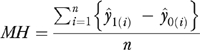(2)

where denotes the modified two-part regression predicted value of U-Rx for the ith individual in coverage scenario obtained using the second- and third-stage estimates. Note that (2) overcomes the observability constraint discussed earlier in that it incorporates unbiased predictions of U-Rx for the counterfactual (unobservable) coverage scenarios. For example, for individuals observed without C-Rx, (2) incorporates an unbiased prediction of U-Rx as it would have been if coverage were given to them. Further details of the estimation method are provided at (See Appendix online).

RESULTS

The characteristics of the study sample are presented in Table 1. In 1999, approximately 80 percent of noninstitutionalized Medicare beneficiaries with some form of Medicare supplementation had prescription coverage. The average number of prescription fills on behalf of this population was 24. The sociodemographic and health characteristics of the sample follow closely that of the Medicare population as a whole. Beneficiaries are predominantly white, female, married, with a high prevalence of hypertension, arthritis, and heart disease. The bottom panel of the table presents sample means for the seven instrumental variables.

Table 1.

Descriptive Statistics for the Study Sample of Community-Dwelling Medicare Beneficiaries in 1999 (N = 5,270)

Variable	Mean or % of Sample
Number of prescriptions filled/refilled	23.8
Prescription coverage (C-Rx)	80.2%
Age	73.30
Midwest	20.3%
West	26.6%
South	33.5%
Female	55.4%
Metro	78.7%
Income	$30,281
Black	8.3%
Married	56.9%
High school graduate	30.4%
Some college	41.8%
Heart disease	44.3%
Cancer	34.8%
Arthritis	62.4%
Lung disease	14.8%
Psychiatric disorders	8.6%
Alzheimer's disease	2.1%
Diabetes	16.2%
Hypertension	58.5%
Osteoporosis/bone disease	14.3%
Stroke	11.7%
Excellent health	14.8%
Very good health	28.3%
Good health	32.0%
ADL	0.6
IADL	0.3
DCG/HCC risk adjuster	$4,693
Instrumental Variables
% State workforce unionized	14.7%
Mean annual state-level Medigap premium (H, I, J plans)	$2,140
State requires community rating of Medigap premiums	10.8%
State offers expanded benefits to QMB recipients	20.5%
State has pharmaceutical assistance plans	32.1%
State offers Medicaid medically needy coverage	74.0%
State per capita income	$28,741

ADL, limitations in activities of daily living; IADL, limitations in instrumental activities of daily living; DCG/HCC, Diagnostic Cost Group/Hierarchical Condition Category.

Table 2 presents results from the first-stage probit estimation for selection into prescription coverage. Note that the Wald statistic for the identifying instruments (the last seven variables in Table 1) is 47.1, which suggests that they are jointly predictive of prescription coverage at the individual level. As discussed previously, we include RESID as an additional regressor in the estimation of both parts of the modified two-part utilization model to correct for unobservable confounding in the second and third stages of the estimation. As an alternative means of correcting for confounding we include the DCG/HCC risk adjuster as a regressor in the modified two-part model. In order to evaluate the effectiveness of these two approaches to correcting for health-related endogeneity taken individually and in combination, we estimated four distinct versions of the model—one for each of the four possible variable inclusion configurations with respect to the RESID and the DCG/HCC risk adjuster.

Table 2.

First-Stage Probit Estimates Predicting Prescription Drug Coverage (C-Rx)

Variable	Coefficient	t-Statistic
Constant	−0.701	−1.929
Age	−0.001	−0.639
Midwest	0.244	2.609
West	0.162	1.463
South	0.109	0.900
Female	0.072	1.563
Metro	0.163	2.985
Income	1.12 × 10−6	1.672
Black	−0.158	−2.073
Married	0.184	4.025
High school graduate	0.107	1.940
Some college	0.101	1.867
Heart disease	0.184	4.047
Cancer	0.112	2.453
Arthritis	0.189	4.267
Lung disease	0.103	1.610
Psychiatric disorders	0.178	2.071
Alzheimer's disease	0.307	1.739
Diabetes	0.204	3.202
Hypertension	0.390	9.000
Osteoporosis/bone disease	0.104	1.588
Stroke	0.062	0.859
Excellent health	−0.291	−3.921
Very good health	−0.036	−0.553
Good health	0.082	1.328
ADL	−0.012	−0.551
IADL	−0.015	−0.499
DCG/HCC risk adjuster	3.46 × 10−5	5.686
Unionization	−0.016	−2.651
Medigap premium	0.000	3.406
Medigap law	−0.137	−1.452
QMB plus	0.306	3.944
Pharmaceutical assistance plans	0.171	1.773
Medicaid medically needy coverage	0.018	0.316
Per capita income	8.69 × 10−7	0.889

ADL, limitations in activities of daily living; IADL, limitations in instrumental activities of daily living; DCG/HCC, Diagnostic Cost Group/Hierarchical Condition Category.

Results from the second-stage probit estimation for all four versions of the hurdle component of the modified two-part model are given in Table 3. Third-stage NLS results for the levels component in each of the four model variants are displayed in Table 4. These estimates constitute the intermediate step in estimating the MH effect and, as such, are generally of no policy interest. A few of the parameter estimates are, however, noteworthy. First note that the coefficient of prescription coverage is positive and highly significant in both parts of all four models. This fact will later be reflected in the positive and significant estimates that we obtained for the MH effects. When RESID is included and DCG/HCC is excluded from the model, we find evidence of endogeneity as indicated by the statistically significant coefficients of RESID in both parts of the model (p-values less than 6 and 5 percent, respectively). This shows that our estimator is accounting for the omitted variable bias due to the exclusion of DCG/HCC. Likewise, under the opposite inclusion configuration (DCG/HCC in, RESID out), there is evidence that the risk adjuster is accounting for confounding due to health status. In this case the coefficient of DCG/HCC is insignificant in the hurdle component of the model, but highly significant in the levels part of the model. When both RESID and DCG/HCC are included in the model neither has a statistically significant coefficient in the first part of the model but both are statistically significant in the second part of the model (at the 5 and 1 percent levels, respectively). Overall, it appears that confounding is a problem, and both RESID and DCG/HCC play distinct and complementary roles in correcting for it.

Table 3.

Four Probit Estimates of Any Drug Use Based on Alternate Inclusion Rules for DCG/HCC and RESID

	(1) Neither DCG/HCC nor RESID		(2) RESID Only		(3) DCG/HCC Only		(4) Both DCG/HCC and RESID
Variable	Coefficient	t-Statistic	Coefficient	t-Statistic	Coefficient	t-Statistic	Coefficient	t-Statistic
Constant	−1.054	−3.550	−1.064	−3.423	−1.065	−3.576	−1.067	−3.580
Age	0.003	0.966	0.004	0.982	0.003	0.818	0.003	0.806
Midwest	0.111	0.921	0.125	0.992	0.111	0.922	0.112	0.932
West	−0.091	−0.852	−0.083	−0.757	−0.089	−0.833	−0.088	−0.825
South	0.179	1.642	0.199	1.738	0.177	1.625	0.179	1.638
Female	0.325	3.937	0.329	3.804	0.328	3.967	0.329	3.971
Metro	−0.070	−0.741	−0.050	−0.508	−0.066	−0.695	−0.063	−0.665
Income	2.29 × 10−6	1.600	2.04 × 10−6	1.757	2.06 × 10−6	1.614	2.08 × 10−6	1.625
Black	−0.342	−2.662	−0.366	−2.744	−0.340	−2.652	−0.343	−2.664
Married	0.184	2.228	0.203	2.342	0.190	2.281	0.193	2.298
High school graduate	0.255	2.624	0.268	2.634	0.255	2.618	0.256	2.628
Some college	0.293	3.051	0.309	3.078	0.291	3.023	0.293	3.034
Heart disease	0.404	4.369	0.434	4.303	0.402	4.348	0.404	4.356
Cancer	0.231	2.585	0.253	2.645	0.231	2.582	0.233	2.595
Arthritis	0.165	2.099	0.185	2.240	0.168	2.132	0.171	2.151
Lung disease	0.368	2.553	0.389	2.439	0.365	2.530	0.367	2.537
Psychiatric disorders	−0.024	−0.149	0.008	0.045	−0.024	−0.148	−0.022	−0.135
Alzheimer's disease	−0.476	−1.581	−0.364	−1.129	−0.470	−1.554	−0.463	−1.528
Diabetes	0.613	3.897	0.659	3.603	0.612	3.887	0.616	3.891
Hypertension	0.748	8.830	0.803	8.263	0.748	8.837	0.754	8.694
Osteoporosis/bone disease	0.364	2.414	0.384	2.286	0.364	2.412	0.365	2.418
Stroke	−0.153	−1.031	−0.141	−0.890	−0.154	−1.039	−0.152	−1.026
Excellent health	−0.209	−1.664	−0.249	−1.885	−0.188	−1.430	−0.190	−1.445
Very good health	−0.071	−0.608	−0.086	−0.699	−0.053	−0.432	0.053	−0.433
Good health	0.114	0.956	0.117	0.931	0.130	1.058	0.131	1.066
ADL	0.070	1.594	0.068	1.441	0.069	1.579	0.069	1.570
IADL	0.079	1.208	0.076	1.072	0.078	1.200	0.078	1.194
DCG/HCC risk adjuster	—	—	—	—	0.605 × 10−5	0.534	0.695 × 10−5	0.590
Prescription coverage	2.106	23.910	2.076	20.365	2.100	23.686	2.096	23.435
RESID	—	—	0.020	1.942	—	—	0.002	0.308

ADL, limitations in activities of daily living; IADL, limitations in instrumental activities of daily living; DCG/HCC, Diagnostic Cost Group/Hierarchical Condition Category; RESID, first-stage probit residual.

Table 4.

Four NLS Estimates of Number of Annual Drug Fills Conditional on Any Drug Use Based on Alternate Inclusion Rules for DCG/HCC and RESID

	(1) Neither DCG/HCC nor RESID		(2) RESID Only		(3) DCG/HCC		(4) Both DCG/HCC and RESID
Variable	Coefficient	t-Statistic	Coefficient	t-Statistic	Coefficient	t-Statistic	Coefficient	t-Statistic
Constant	2.533	−36.418	2.445	17.462	2.556	−37.115	2.528	19.049
Age	−0.002	−1.298	−0.002	−1.059	−0.003	−2.093	−0.004	−2.241
Midwest	0.101	2.692	0.108	3.108	0.105	2.822	0.108	3.169
West	−0.095	−2.468	−0.091	−2.455	−0.073	−1.907	−0.069	−1.833
South	0.146	4.323	0.165	5.067	0.150	4.409	0.157	4.733
Female	0.168	5.801	0.175	6.372	0.182	6.085	0.188	6.427
Metro	0.017	0.578	0.043	1.398	0.018	0.609	0.028	0.852
Income	7 × 10−8	0.252	1.47 × 10−7	0.466	7 × 10−7	0.256	8.02 × 10−8	0.426
Black	−0.104	−1.859	−0.129	−2.425	−0.112	−1.923	−0.116	−2.039
Married	0.052	1.850	0.070	2.746	0.053	1.923	0.061	2.431
High school graduate	0.0001	0.005	0.011	0.470	−0.007	−0.224	−0.005	−0.085
Some college	0.002	0.079	0.018	0.867	−0.006	−0.192	−0.003	0.166
Heart disease	0.261	10.201	0.286	11.415	0.252	9.848	0.257	10.437
Cancer	−0.021	−0.834	0.004	0.498	−0.030	−1.205	−0.023	−0.623
Arthritis	0.116	4.316	0.134	5.377	0.134	4.902	0.141	5.542
Lung disease	0.194	6.096	0.215	7.145	0.187	5.915	0.185	6.061
Psychiatric disorders	0.143	3.475	0.178	4.433	0.159	3.906	0.163	4.049
Alzheimer's disease	0.009	0.101	0.115	1.377	0.021	0.246	0.038	0.472
Diabetes	0.214	7.166	0.260	8.094	0.181	5.985	0.192	6.482
Hypertension	0.265	9.236	0.302	10.977	0.260	9.081	0.267	10.337
Osteoporosis/bone disease	0.072	2.153	0.088	2.831	0.071	2.152	0.077	2.530
Stroke	0.039	1.072	0.049	1.271	0.024	0.662	0.022	0.506
Excellent health	−0.394	−8.193	−0.420	−8.991	−0.356	−7.249	−0.350	−7.389
Very good health	−0.290	−8.982	−0.303	−9.609	−0.255	−7.767	−0.251	−7.763
Good health	−0.147	−5.025	−0.147	−5.058	−0.123	−4.143	−0.118	−3.923
ADL	0.041	3.783	0.040	3.853	0.034	3.137	0.034	3.166
IADL	0.039	2.377	0.036	2.236	0.031	1.940	0.030	1.968
DCG/HCC risk adjuster	—	—	—	—	1.28 × 10−5	5.327	1.64 × 10−5	5.454
Prescription coverage	0.351	8.339	0.341	13.063	0.336	8.149	0.333	13.202
RESID	—	—	.007	3.065	—	—	0.001	1.823

ADL, limitations in activities of daily living; IADL, limitations in instrumental activities of daily living; DCG/HCC, Diagnostic Cost Group/Hierarchical Condition Category; RESID, first-stage probit residual.

The estimates of MH in the four versions of the modified two-part model are given in Table 5. These estimates are obtained through appropriate application of the DOM statistic given in (2). The t-statistics are displayed in parentheses and 95 percent confidence intervals are given in brackets. All estimates are positive and statistically significant at any reasonable level. The consequences of failing to correct for endogeneity are clearly manifested in Table 5. As expected, the version of the model that neglects endogeneity (neither RESID nor DCG/HCC included) yields a MH estimate that is larger than the other three configurations. In this case, the DOM estimator is biased because it spuriously picks up influences that are actually due to latent selection factors. Both of the models underlying the off-diagonal cells in Table 5 attenuate this bias, though the specification which only includes RESID appears to be more effective in this regard. The RESID-only estimate of the MH (11.26) is very close to the estimate that accounts for both RESID and DCG/HCC (11.22), a difference of 0.04 prescriptions. In comparison, the DCG/HCC only estimate (11.30) exceeds the RESID and DCG/HCC combined estimate by double that amount.

Table 5.

Estimated Increase in Prescription Drug Fills per Year Due to Prescription Coverage (The Moral Hazard Effect)

	No DCG/HCC (Asymptotic t-Statistics) [95% Confidence Intervals]	DCG/HCC Included (Asymptotic t-Statistics) [95% Confidence Intervals]
No RESID	11.56 (16.92) [10.221, 12.9]	11.30 (16.62) [9.967, 12.633]
RESID included	11.26 (16.20) [9.898, 12.622]	11.22 (16.47) [9.89, 12.556]

RESID, first-stage probit residual.

Using the formula presented in Moffitt (2006), we calculate the arc elasticity of prescription drug demand from the RESID and DCG/HCC model to be −0.54; that is to say, given a 10 percent reduction in the effective price of medications to beneficiaries, drug utilization is projected to rise by 5.4 percent. Elasticities calculated for the other model results shown in Table 5 differ from this estimate by less than 0.05.

DISCUSSION

There are several findings to note from this study. First, all else being equal, Medicare beneficiaries with full-year drug coverage have significantly higher medication utilization rates compared with those with no drug coverage. Our elasticity estimate of −0.54 is at the upper range of previous estimates based on older data and methods. The slightly higher estimate may be the result of these differences in data and methods as well as to changes in the pharmaceutical market in 1990s, such as a large number of new drug approvals and innovations in marketing directly to consumers. Even this slightly higher elasticity estimate, however, can lead to significant changes in the cost of the benefit (Shea, Stuart, and Briesacher 2003/2004).

Second, even before the advent of Part D, we find evidence of selection in our first-stage estimates of prescription drug coverage. In the study year, beneficiaries in excellent health status were much less likely to have drug coverage; those with common chronic conditions and high predicted Medicare spending (from the DCG/HCC) were more likely to have coverage.

Third, although we find some evidence of selection based on nonobservable factors (the RESID results), the estimated magnitude of the effect is small. As a consequence, we find a close correspondence in estimates of moral hazard in drug demand between models with strong covariate control for observable health characteristics and those with residuals derived from instrumental variable estimators. This finding is important from a policy perspective as it suggests that the most important factors underlying the selection process can be captured through information in beneficiaries' Medicare claims files, and to that extent can be managed through risk adjustment.

These conclusions should be interpreted in the light of several important caveats. First, we estimate the impact of drug coverage on the quantity of use not drug expenditures. It should be noted that the authors conducted a parallel analysis using drug expenditures as the dependent variable and generated much higher estimates of the MH effect (not shown). We ascribe these findings to an artifact in the way the MCBS imputes transaction prices for drugs purchased through third-party contracts (based on published estimates of average discounts off average wholesale price) and the transaction prices faced by uninsured beneficiaries paying on a cash basis (where imputations are based on the self reports of respondents with complete payment records). This artifact does not affect MCBS reported counts of drugs used.

A second caveat is that our estimates are derived from a single annual cross-section in which our primary measure of health status, the DCG/HCC risk adjuster, is measured contemporaneously with drug use, not in the form of a lagged predictor as the DCG/HCC is employed in actual practice. In prior work we demonstrated that concurrent and lagged DCG/HCC measures performed almost as well in predicting drug use and spending for Medicare beneficiaries (Wrobel et al. 2003), but it remains to be seen how the newer drug-specific risk adjuster for Part D, the RxHCC, will perform in this regard.

Third, our results must be interpreted in light of two important sample restrictions. We excluded persons with part year drug benefits because the MCBS does not permit mapping drug utilization to periods with and without coverage during the year. We also excluded persons with drug benefits but no Medicare supplementary medical insurance policy. We did this to isolate the independent effect of drug coverage for individuals who have supplementation for the Part B deductibles and coinsurance for physician services.

A final caveat is that the current market for PDPs under Part D is far different than that in our study year, 1999. Beneficiaries today are actively encouraged to select the plan that best meets their own financial and medication needs. Future research will need to assess whether this selection process can be predicted on observable health characteristics or not.

SUPPLEMENTARY MATERIAL

The following supplementary material for this article is available online:

Appendix

Details of the Estimation Method

REFERENCES

- Briesacher B, Stuart BC, Doshi J, Wrobel M. Medicare Beneficiaries and the Impact of Gaining Prescription Drug Coverage on Inpatient and Physician Spending. Health Services Research. 2005;40(5, part 1):1279–96. doi: 10.1111/j.1475-6773.2005.00432.x. [DOI] [PMC free article] [PubMed] [Google Scholar]
- Centers for Medicare and Medicaid Services. The MCBS web page. [accessed on May 16, 2006]. Available at http://www.cms.hhs.gov/apps/mcbs/
- Coulson NE, Stuart BC. Insurance Choice and the Demand for Prescription Drugs. Southern Economic Journal. 1995;61(4):1146–58. [Google Scholar]
- Coulson NE, Stuart BC, Terza J, Neslusan C. Estimating the Moral Hazard Effect of Supplemental Medical Insurance in the Demand for Prescription Drugs. American Economic Review—Papers and Proceedings. 1995;85(2):122–6. [PubMed] [Google Scholar]
- Doshi J, Brandt N, Stuart BC. Impact of Drug Coverage on COX-2 Inhibitor Use in Medicare. Health Affairs. 2004 doi: 10.1377/hlthaff.w4.94. Web exclusive, February 19, 2004. Available at http://content.healthaffairs.org/cgi/content/abstract/hlthaff.w4.94. [DOI] [PubMed] [Google Scholar]
- Feldman R, Dowd B. Must Adverse Selection Cause Premium Spirals? Journal of Health Economics. 1991;10(3):349–57. doi: 10.1016/0167-6296(91)90035-l. [DOI] [PubMed] [Google Scholar]
- Lillard LA, Rogowski J, Kington R. Insurance Coverage for Prescription Drugs. Medical Care. 1999;37(9):926–36. doi: 10.1097/00005650-199909000-00008. [DOI] [PubMed] [Google Scholar]
- Moffitt M. A Primer on Arc Elasticity. 2006 [accessed on May 16, 2006]. Available at http://economics.about.com/cs/micfrohelp/a/arc_elasticity_2.htm.
- Mullahy J. Much Ado about Two Reconsidering Retransformation and the Two-Part Model in Health Econometrics. Journal of Health Economics. 1998;17(3):247–81. doi: 10.1016/s0167-6296(98)00030-7. [DOI] [PubMed] [Google Scholar]
- Pauly M. Medicare Drug Coverage and Moral Hazard. Health Affairs. 2004;23(1):113–22. doi: 10.1377/hlthaff.23.1.113. [DOI] [PubMed] [Google Scholar]
- Pope G, Kautter C, Ellis J, Ash RP, Ayanian AS, Iezzoni JZ, Ingber LI, Levy MJ, Robst J. Risk Adjustment of the Medicare Capitation Payments Using the CMS-HCC Model. Health Care Financing Review. 2004;25(4):119–41. [PMC free article] [PubMed] [Google Scholar]
- Shea DG, Stuart BC, Briesacher B. Participation and Crowd-Out in a Medicare Drug Benefit: Simulation Estimates. Health Care Financing Review. 2003/2004;25(2):47–62. [PMC free article] [PubMed] [Google Scholar]
- Stuart BC, Doshi J, Briesacher B, Wrobel M, Baysac F. Impact of Prescription Coverage on Hospital and Physician Costs A Case Study of Medicare Beneficiaries with Chronic Obstructive Pulmonary Disease. Clinical Therapeutics. 2004;26(10):1688–99. doi: 10.1016/j.clinthera.2004.10.012. [DOI] [PubMed] [Google Scholar]
- Stuart BC, Shea DG, Briesacher B. Dynamics in Drug Coverage of Medicare Beneficiaries Finders, Losers, Switchers. Health Affairs. 2001;20(2):86–99. doi: 10.1377/hlthaff.20.2.86. [DOI] [PubMed] [Google Scholar]
- Stuart BC, Simoni-Wastila L, Baysac F, Shaffer T, Shea DG. Coverage and Use of Prescription Drugs in Nursing Homes Implications for the Medicare Modernization Act. Medical Care. 2006;44(3):243–9. doi: 10.1097/01.mlr.0000199652.15293.fc. [DOI] [PubMed] [Google Scholar]
- Stuart BC, Simoni-Wastila L, Chauncey D. Assessing the Impact of Coverage Gaps in the Medicare Part D Drug Benefit. Health Affairs. 2005 doi: 10.1377/hlthaff.w5.167. Web Exclusive, April 19, 2005. Available at http://content.healthaffairs.org/cgi/content/abstract/hlthaff.w5.167. [DOI] [PubMed] [Google Scholar]
- Terza JV. Parametric Regression and Policy Analysts: A Framework for Estimation and Inference. 2006. Working Paper, Department of Epidemiology and Health Policy Research, Department of Economics, University of Florida.
- Wolfe JR, Goddeeris J. Adverse Selection, Moral Hazard, and Wealth Effects in the Medigap Insurance Market. Journal of Health Economics. 1991;10(4):433–59. doi: 10.1016/0167-6296(91)90024-h. [DOI] [PubMed] [Google Scholar]
- Wrobel M, Doshi J, Stuart BC, Briesacher B. Predictability of Drug Expenditures for Medicare Beneficiaries. Health Care Financing Review. 2003;25(2):37–46. [PMC free article] [PubMed] [Google Scholar]
Associated Data
This section collects any data citations, data availability statements, or supplementary materials included in this article.
Supplementary Materials