Geometries of knowledge

Abstract

It is argued that knowledge representations formalized through pattern theoretic structures are geometric in nature in the following sense. The configurations and resulting patterns appearing in such representations exhibit invariances with respect to the similarity groups and are characterized topologically through their connection types. Starting with a special pattern from microbiology, it is shown how the basic pattern theoretic concepts are introduced in general and what their function is in representing knowledge. Variance/invariance of the patterns is discussed in geometric language. The measures on the configuration spaces are implemented by difference/differential equations which are used as a basis for computer algorithms.

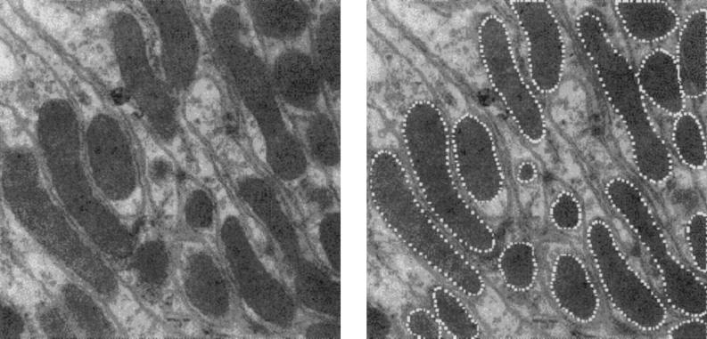
Information and Knowledge. Fig. 1 Left is a micrograph of a cardiac cell in a rat. In it several types of structures can be seen, among them some oblong areas, sometimes oval, sometimes curved, the mitochondria of the cell. The mitochondria, whose functions include supplying energy for the cell, can be seen to vary a good deal between each other. Nevertheless they exhibit some stability: their size, while variable from one to another, is of the same order of magnitude, and their texture is characteristic and different from that of the surrounding cytoplasm.

Figure 1.

(Left) Micrograph of rat cardiac cell. (×20,000.) (Right) Same section, with mitochondria outlined.

These statements could be made more precise and given quantitative form in terms of lengths, areas, intensities and so on, as is customary in biological/medical research. It is less obvious how to assert that the shape also has some stability, how the concept of shape should be formalized in quantitative form without introducing unrealistic assumptions stipulating a fixed form for all the mitochondria.

This difficulty is not limited to mitochondria, nor to microbiology, since the notion of shape pervades biology in general. In brain research, for example, the anatomies are described through basic units like midbrain, ventricles, hippocampus, … , all the way down to the level of cell types as in Brodman’s classical brain map. Or, going in the opposite direction, starting with cells, the anatomist builds larger structures which themselves are combined into even larger units until the entire organism has been accounted for.

During this building process, in which successive levels are introduced, with units that are measured and located with respect to each other, it is practical to express the descriptive anatomical statements in some coordinate system. It is clear that, the relations should be invariant with respect to the Euclidean group of transformations.

A large collection of such micrographs contains a lot of information in raw form about mitochondria, but it is only when information is organized into ordered systems that it becomes knowledge, say in the form of a textbook, or a theory, a doctrine. To fix ideas we shall limit ourselves to discussing the form of mitochondria, but the reasoning is of much greater generality.

Before entering this discussion it is reasonable to ask why such representations are needed. Say that a biologist has accumulated evidence about some organism, for example in the format of pictures such as the one in Fig. 1. If the number of pictures is small they can be examined “manually” one by one, and the raw data can be reduced to quantitative measurements and summarized into meaningful statements. When the observational techniques become increasingly automated the researcher will be faced by mountains of data and it is reasonable to turn to computational methods of analysis. But to develop computer programs for such a task requires that it be formulated in exact terms: the computer is unforgiving when it comes to nebulous or ambiguous instructions. We are thus forced to formalize our understanding of the research object in well defined logical categories so that they can be correctly translated into computer code: we need, indeed, a formal representation of the knowledge.

To represent knowledge by doctrines, perhaps by mathematical models, has a long history going back to the dawn of scientific thinking. Sometimes this has resulted in highly concise theories of great beauty; Newtonian mechanics is the example par preference. Others are differently expressed, not using mathematical terminology but nevertheless organizing a mass of information into knowledge representations; the botanical taxonomy of Linnaeus could serve as an example. It is when we are confronted by really complex systems, heterogeneous, highly variable, and with complicated interactions between their parts, that the need arises for formal structures that has led to the creation of pattern theory. Biology/medicine offers many examples of this.

Knowledge as Geometry.

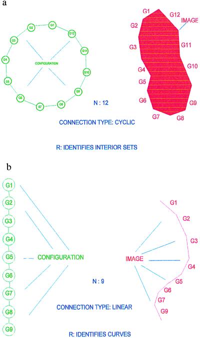
To be more concrete, let us return to the representation of the shape of mitochondria in micrographs. In Fig. 2a we show a polygon whose shape is at least reminiscent of that of a mitochondrion. Let us denote the vertices of an arbitrary polygon, not necessarily closed, see Fig. 2b, by xⁱ = (x₁ⁱ, x₂ⁱ) ∈ R²; i = 1, 2, … , n + 1 and think of the polygon as generated by the n sides

To ensure that the sides are contiguous we introduce bond values

with the obvious bond relation

In this illustrative example the choice of bond relation is obvious but that will not always be the case.

Figure 2.

(a) CYCLIC. (b) LINEAR.

Formally we shall write the representation of the n-gon as a configuration

with σ = LINEAR meaning a connector graph, here just a linear graph. These configurations, constrained by the bond relation, form a configuration space 𝒞 = 𝒞(ℛ), where the symbol ℛ stands for the regularity expressed by the bond relation. The constraints are local in the sense that each one involves only a bounded number, in this case two, of generators as n → ∞. The configuration is interpreted to mean the curve I in the plane corresponding to the polygon and written formally as R : c ↦ I; I = Rc. R is called an identification rule; see below.

We shall also need a subconfiguration space 𝒞(ℛ_closed) consisting of configurations

where the connector graph CYCLIC means that the bond relations are also valid for the bond couple (β_outⁿ, β_in¹). We also ask that the polygon not be self-intersecting, which is a global constraint. If that is assumed to be true, Jordan’s theorem guarantees that the curve divides the plane R² into two regions, the inside I and its complement I^c. We can then interpret the configuration as “meaning” the image I (see Fig. 2a; we use an identification rule

Note that R is not invertible, since an n-gon encloses a set that can also be enclosed by an m-gon, m > n, with some colinear sides. This distinction may at first seem like splitting hairs but is actually fundamental. The representation through a configuration, the deep structure to use Chomsky’s terminology, is not always uniquely determined by the image, the surface structure. This is like the relation between a function and a formula that represents the function: the formula determines the function but not the opposite.

To handle the permanence of the concept of shape we shall specify a group of transformations that induces invariance. The group will in general be called the similarity group, borrowing and extending the meaning of this term from Euclid, and shall act on the space G of generators, in this example

since then a generator is determined by its bondvalues, each of dimension two. A good choice of similarity group here has been shown to be the product of the special plane Euclidean group with that of uniform scale change

where a generic group element s ∈ S acts according to

and extend this definition from G to 𝒞 by

Note that this transformation acts in the same way on all the generators in the configuration—it is a rigid (up to scale change) transformation. But rigid transformations will not suffice for the representation of flexible shape, since they only describe a single polygon translated, rotated, and uniformly scaled, which is clearly insufficient for describing the variability of mitochondria.

To proceed we introduce local transformations of one or several templates. Starting with a template configuration

introduce the deformed template by

with similarities s₁, s₂, … , s_n ∈ S arbitrary except that they make c ∈ 𝒞(ℛ). Then the polygon can undergo more flexible changes and we shall see below how to make this a powerful model of shape.

The image algebra

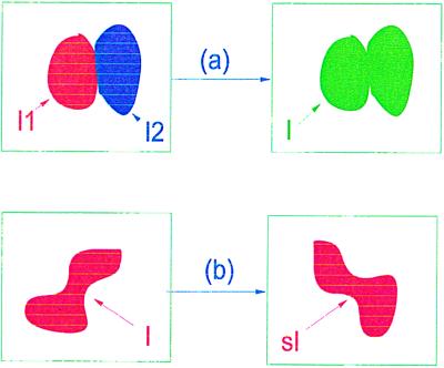
is indeed an algebraic structure and allows two types of operations. First, the rigid similarities s : ℐ → ℐ naturally defined through s : I ↦ sI and, second, combinations of images I₁ = Rc₁; I₂ = Rc₂; c₁, c₂ ∈ 𝒞(ℛ). Let σ be a connector graph that connects unconnected bonds from c₁ to bonds of c₂ and form the configuration

If the new connector is regular, c ∈ 𝒞(ℛ), so that the last outbond of c₁ agrees with the first inbond of c₂, we can form the image I = Rc and write formally I = σ(I₁, I₂) for the second type of algebraic operation in ℐ. We also have the sub-image algebra

representing sets enclosed by polygons as in Fig. 2a. Then we have only one type of algebraic operation, namely I → sI. In Fig. 3 we show some instances of both types of algebraic operations.

Figure 3.

Algebraic operations. (a) Combination. (b) Similarity.

The mapping R : sc_temp ↦ I_temp produces a deformed image template from the deformed configuration template. Further, we can expose any image I to rigid transformations and form the set of images

We shall call P(I) a pattern and the set

of all patterns can then be seen to be the quotient space ℐ/S.

The micrograph in Fig. 1a contains several mitochondria and in general we must take into account the fact that the number is not known beforehand. We do this by extending the choice of connectors: we now allow any connector graph σ consisting of a finite number of cyclic graphs, so that we are dealing with the family of graphs

This leads to the extended configuration space

which the identification rule R makes into the larger image algebra

namely, the union of Cartesian products of the original image algebra, so that k is the number of mitochondria in the image.

The way in which we represent knowledge relative to groups of transformations inducing invariances is reminiscent of Felix Klein’s celebrated Erlangen program (1), in which he suggested that geometries should be viewed as systems in which certain relations are invariant with respect to some group of transformations. We can therefore speak of pattern theory as a geometry of knowledge, and we can view configurations as geometric objects. Also, the connector graph, which in general can be quite complicated, describes the neighborhood relations of the knowledge representation which gives rise to a topology of the knowledge representation. Hence we are faced by problems in geometry, albeit of nontraditional type.

Representing Variability in a Flexible Geometry.

The image algebra ℐ_closed has enough flexibility to represent mitochondria shape. Actually, it can represent very complicated shapes quite different from those of mitochondria: it is too general and must be restricted to be useful.

To do this we introduce measures on the configuration space and image algebra that will describe normal variability of the shapes. One could define such measures directly on 𝒞 or ℐ but it is more natural to do it for the similarities s₁, s₂, … , s_n that give rise to the deformed templates, since this reduction brings us closer to the morphogenesis that produces shape. In other words we shall introduce a measure m on Sⁿ with the intent that m will emphasize the shapes that occur most commonly in nature but give little weight to others.

We shall usually choose m to be bounded so that we can normalize it to a probability measure

with the normalization constant Z = m(Sⁿ) known as the partition function to the physicist. The actual construction of m will of course depend upon the particular knowledge domain that is to be represented but should agree with the topology of that domain in the following sense.

For simplicity, say that S is finite-dimensional Euclidean space and that m will be given in terms of a density f on Sⁿ with respect to Lebesgue measure dsⁿ on Sⁿ. We shall ask that the density, the Radon–Nikodym derivative, have the multiplicative form

with the convention n + 1 ≡ 1. The function A(·, ·), the acceptor function, controls the dependence between the similarity transformations applied to the n generators.

In the special case of mitochondrial shapes, the following specification of the acceptor function has been used successfully. Consider a similarity acting upon a generator g = (β_in, β_out) ∈ R⁴ as

with the translation parameter a ∈ R², the rotation angle φ ∈ [0, 2π), and the scaling factor r > 0, we can read the scaling/rotation part as polar coordinates as

with u, v ∈ R. On the four-dimensional similarity group S parametrized by a₁, a₂, u, v we define an acceptor function

with the quadratic forms

The rationale behind this choice of A(·, ·) is, first, that we want its maximum to be achieved for a₁ = a₂ = 0 and u = 1, v = 0 implying r = 1, φ = 0, in other words at the identity of the group S = SE(2) × SU(2). Second, we need to control the variability of the boundary ∂I which we do by means of the variability parameters σ_location, σ_u, σ_v that express how much changes in the location, orientation, and scaling will deviate from the identity. Third, we must also control the smoothness of ∂I through the smoothness parameters ρ_location, ρ_u, ρ_v—by making them small the boundary will be more chaotic and vice versa.

This defines a density and measure on 𝒞(ℛ), and we shall restrict it to the sub-configuration space 𝒞(ℛ_closed) by constraining the measure to that manifold, in this example of dimension 2n instead of 4n for the unrestricted configuration space. Leaving out the technicalities about how to do this, note only that one has to describe the variability of k, the number of mitochondria in the image. This is going to result in a total measure consisting simply of a linear combination

unless we want to exclude the possibility of two mitochondria overlapping each other, which will not be discussed here.

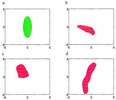
But how does this actually work, how well does the knowledge representation mirror the shape properties of real mitochondria? This question can be answered in two ways, one of which is pattern synthesis. If we use Monte Carlo simulation of the representation with appropriate values plugged in for the variability parameters, how do the images look? Fig. 4 shows an empirical template in green and some synthesized shapes in red; they seem to be at least qualitatively like the ones in Fig. 1. But this is not the deciding test for whether to accept or reject the representation. Instead we will have to study how it behaves when applied to real micrographs, pattern analysis, and this will be discussed below in Differential Equations for Patterns. But first I shall put the previous in a more general perspective.

Figure 4.

(a) Template. (b–d) Synthesized shapes.

Geometry of Patterns in Complex Systems.

The previous discussion was all in a very special case, but the treatment of patterns in a general system can be based on the same concepts and reasoning. The abstract formulation, abbreviated by omitting some topics that are important but cannot be treated here, reads as follows; more precise statements and proofs can be found in Grenander (ref. 2, chapters 1 and 2 and part IV, and ref. 3).

Starting from a generator space G of primitive objects equipped with a number, the arity ω(g), of bond values

with values in some bond value space B, and a bond relation

we form configurations

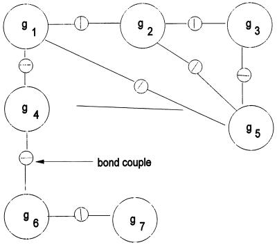
by putting the generator g_i at the ith site of the connector graph σ from some family, the connection type, Σ, of connector graphs. A group S of transformations s : G → G acts on G. In most cases that have been analyzed S is a finite-dimensional Lie group. The configuration c is said to be ℛ-regular with the regularity

if all pairs of bonds emanating from two sites (i₁, i₂) connected by σ satisfy the bond relation

and σ ∈ Σ. See Fig. 5. The regularity ℛ leads to a configuration space 𝒞(ℛ) and, with some equivalence relation R, the identification rule, we get the image algebra as the quotient

Figure 5.

Configuration diagram.

and the pattern family

The regularity ℛ determines the geometry of the knowledge represented by the regular structures 𝒞(ℛ) and together with the identification rule R it determines also the algebraic structure of ℐ.

Returning to the configuration space, we introduce a measure m as a Radon–Nikodym derivative with respect to a σ-finite measure μⁿ on Sⁿ through the structure formula

with some acceptor function

and the product taken over all pairs (i₁, j₁) ↔ (i₂, j₂) connected by the graph σ. When S is a Lie group it is natural to choose the measure μⁿ as an invariant measure on the group. The measure m induces measures on the image algebra ℐ and patterns in 𝒫 just as in the mitochondria example. If the measure m is bounded it can be made into a probability measure by normalizing with the partition function Z = m(𝒞(ℛ)). These measures determine the metric structure of the knowledge representations.

Differential Equations for Patterns.

Once we have acquired some understanding of the geometry of a pattern class it can be exploited for practical use. It then depends upon what sensor was used to acquire the picture. Medical sensor technology has advanced rapidly in recent years and resulted in a multitude of modalities—for example, magnetic resonance, ultrasound, positron emission tomography, and visible light microscopy to mention but a few. The micrographs in the first section of this paper were obtained by an electron microscope, and we shall discuss the analysis of them, pointing out that the mathematical method is essentially the same for all modalities except, of course, that the physics can differ radically from one sensor to another.

Call the observed image deformed by biological variability as well as by sensor imperfections I^𝒟. In most cases the deformed image can be represented by an array so that we can write

where Y stands for the array and its entries of I^𝒟 are real numbers. One can make this concrete by thinking of Y as parametrizing the “photographic plate” taking this term in a wide sense. The biological variability is described by a prior probability density π(c) as discussed in the previous section, and we now have to describe the sensor physics by another probability density L(y|c) conditioned by the statement that c = sc_temp is the true configuration. The form of L(·|·) will vary from sensor to sensor, and I only offer a simple example when Y is a square matrix and I is a subset of the square (0, l)²

with the sums extended over the subsets of the l × l lattice

The typical intensity inside an object is m_in and outside m_out. The resolution of the sensor is measured by the value of l and its accuracy by σ_obs.

Introduce the functions of sⁿ, called energies because of their role similar to that of real energies in physics,

In this approach all the knowledge about the unknown true configuration c is contained in the prior knowledge represented by π(·) and the empirical knowledge represented by I^𝒟 and can be summarized by the posterior densisty

This is just Bayes’ theorem when the deformed image I^𝒟 is treated as observed and fixed. The problem of how to make strong statements about the pattern represented by the unknown sⁿ, c, or I is therefore reduced to handling p(sⁿ|I^𝒟).

To do this we shall employ the differential equation

involving the gradient ∇E(sⁿ) and the Wiener process W(·) on the Lie group S. The variable t denotes algorithmic time.

This differential equation can be motivated in two ways. The first, simple but superficial, is to point out that the first term on the right makes the trajectory through Sⁿ move against the gradient of the energy E(sⁿ) so that it tends toward a local energy minimum. Many systems in the physical sciences are controlled by such a behavior, so it is not unreasonable to postulate this sort of strategy for interpreting an observed image.

A deeper motivation is to consider the probability measure P(t) of sⁿ(t) and to note the well known fact that

as t → ∞, where P is the measure with density p(sⁿ|I^𝒟). That means that if we solve the differential equation from t = 0 up to a large value t_final, then the resulting value

so that sⁿ(t_final) is a likely explanation of I^𝒟. Doing this a number of times will give us a sense of what accuracy we can attach to the explanation. Many variations of this statement can be made, but the above one will have to suffice here. We shall bypass a technical difficulty, ergodicity, here and only refer to Grenander and Miller (4).

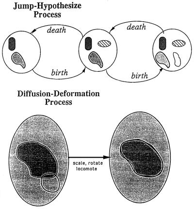
Of course the variability of k, the number of mitochondria in a micrograph, must also be taken into account. Without entering into a discussion of how this has been done we just mention that the differential equation will be extended to a difference-differential equation for which the solution is allowed to jump at discrete time points corresponding to the decision k → k ± 1 and follow the differential equation between the jumps. Fig. 6 shows schematically how the solution develops through configuration space.

Figure 6.

Solution development.

In the mitochondria study the output of the differential-difference equation can look like Fig. 1 Right, which shows the boundaries of the recognized mitochondria.

Let us now turn to a more challenging task, to represent variability in images obtained by magnetic resonance, positron emission tomography, or single photon emission computed tomography. Here too the formulations should start in the Euclidean continuum, not on the lattice of the observed picture as has often been done in traditional pattern recognition, which is one of the reasons for its difficulties. We are now in R³. Configurations are then built from generators consisting of the components of the brain, hierarchically organized, and with bondvalues made up from surface patches. Further, the generators may carry parameters—for example, indicating tissue type or the name of the component. The connectors, the σs, that represent the topology of anatomical atlases, say for normal anatomies, express contiguity of surface patches.

For (normal) anatomical patterns the similarity transformations will be made up of a cascade of groups. On each group in the cascade a measure is introduced to represent that part of the variability that is due to the transformations in the group. This leads to a density p(c|I^𝒟) by an argument that is in principle the same as the one above, although more complicated, and also to differential equations over the respective groups.

Given a template brain represented by a configuration

we acquire for a patient an observed image I^𝒟 and then solve the differential equations to find a reasonable diffeomorphism d* : I_temp → ℐ that will serve as an explanation of the observation. We then let d* operate on the generators in the image template

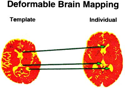
This makes it possible to achieve automatic recognition of the components of the patient brain as Rd*g_i. Fig. 7 indicates the nature of such automatically obtained mappings, or brain warps. Once the components have been identified it is a simple matter to let the computer calculate their volumes, areas, and curvatures, as well as other geometric characteristics that may be of help to correlate with the symptoms and signs observed for the patient.

Figure 7.

Deformable brain mapping.

Of course this procedure is justified only for a patient population with brains topologically equivalent to I_temp. With conscious abuse of medical terminology we name a brain normal only if it is topologically equivalent to the template in the given sub-population; this we consider a necessary (but not sufficient) condition for normality. How to deal with images of abnormal brains requires an extension of the methodology described above, but we cannot go into this challenging topic here.

Geometric Understanding of Patterns.

We have argued that pattern theoretic representations of knowledge are inherently geometric in nature. Their geometry is described metrically by transformations from Lie groups, the similarities S. They are described topologically by graph structures Σ and jump transformations acting upon these connection types. With the aid of such variability transformations questions of inference from observed images reduce to the geometric understanding of the pattern. The two examples discussed above happened to be pictorial; this was completely incidental, however, and the statement is not limited to understanding of observed pictures.

Such understanding is possible for patterns of general nature by solving the differential equation that governs the system and is derived from a pattern theoretic representation. The aim of these knowledge representations is fundamentally different from that in artificial intelligence, AI, in which the same term occurs. In AI the overall objective is to imitate human intelligence in general by computer algorithms. The goal of pattern theory, on the other hand, is at the same time more limited and more ambitious. It is limited in that it does not pretend to be able to imitate general intelligence, only narrow segments of human mental activities such as recognition of mitochondria or anatomical components. It is ambitious in that it tries to automate such activities so that the task can be carried out faster and perhaps better than by humans.

But this approach is also limited to really complex systems, where it is important to realize that “complex” does not just mean big but has a more restricted meaning. A system with lots of components, such as an ideal, monatomic gas, is certainly complicated, and its study has raised challenging mathematical questions. Nevertheless the rules that are assumed to govern its behavior are straightforward and no pattern formalism is needed—it would help little if at all. In contrast, systems in biology/medicine often exhibit behavior characterized by a high degree of heterogeneity, complicated interactions, and awesome variability. Then a formal representation helps to separate the essential from the incidental and sets the mathematical stage for a rational approach to automated image understanding in the limited sense above. The last decade has witnessed the successful application of this methodology to microbiology, digital anatomy, language theory, and automatic target recognition, and some attempts are being made at present to use these ideas in nonnumerical situations.

References

- 1.Klein F. Math Ann. 1893;43:63. [Google Scholar]
- 2.Grenander U. General Pattern Theory. Oxford: Oxford Univ. Press; 1993. [Google Scholar]
- 3.Miller M I, Christensen G E, Amit Y, Grenander U. Proc Nat Acad Sci USA. 1993;90:11944–11948. doi: 10.1073/pnas.90.24.11944. [DOI] [PMC free article] [PubMed] [Google Scholar]
- 4.Grenander U, Miller M I. J R Stat Soc Ser B. 1994;56:549–603. [Google Scholar]