Optimization of Biomathematical Model Predictions for Cognitive Performance Impairment in Individuals: Accounting for Unknown Traits and Uncertain States in Homeostatic and Circadian Processes

Abstract

Current biomathematical models of fatigue and performance do not accurately predict cognitive performance for individuals with a priori unknown degrees of trait vulnerability to sleep loss, do not predict performance reliably when initial conditions are uncertain, and do not yield statistically valid estimates of prediction accuracy. These limitations diminish their usefulness for predicting the performance of individuals in operational environments. To overcome these 3 limitations, a novel modeling approach was developed, based on the expansion of a statistical technique called Bayesian forecasting. The expanded Bayesian forecasting procedure was implemented in the two-process model of sleep regulation, which has been used to predict performance on the basis of the combination of a sleep homeostatic process and a circadian process. Employing the two-process model with the Bayesian forecasting procedure to predict performance for individual subjects in the face of unknown traits and uncertain states entailed subject-specific optimization of 3 trait parameters (homeostatic build-up rate, circadian amplitude, and basal performance level) and 2 initial state parameters (initial homeostatic state and circadian phase angle). Prior information about the distribution of the trait parameters in the population at large was extracted from psychomotor vigilance test (PVT) performance measurements in 10 subjects who had participated in a laboratory experiment with 88 h of total sleep deprivation. The PVT performance data of 3 additional subjects in this experiment were set aside beforehand for use in prospective computer simulations. The simulations involved updating the subject-specific model parameters every time the next performance measurement became available, and then predicting performance 24 h ahead. Comparison of the predictions to the subjects' actual data revealed that as more data became available for the individuals at hand, the performance predictions became increasingly more accurate and had progressively smaller 95% confidence intervals, as the model parameters converged efficiently to those that best characterized each individual. Even when more challenging simulations were run (mimicking a change in the initial homeostatic state; simulating the data to be sparse), the predictions were still considerably more accurate than would have been achieved by the two-process model alone. Although the work described here is still limited to periods of consolidated wakefulness with stable circadian rhythms, the results obtained thus far indicate that the Bayesian forecasting procedure can successfully overcome some of the major outstanding challenges for biomathematical prediction of cognitive performance in operational settings.

Citation:

Van Dongen HPA; Mott CG; Huang JK; Mollicone DJ; McKenzie FD; Dinges DF. Optimization of biomathematical model predictions for cognitive performance impairment in individuals: accounting for unknown traits and uncertain states in homeostatic and circadian processes. SLEEP 2007;30(9):1129-1143.

INTRODUCTION

REDUCED LEVELS OF ALERTNESS AND DEGRADED COGNITIVE PERFORMANCE DUE TO SLEEP LOSS AND NIGHT WORK ARE A CONCERN IN MANY OPERATIONAL settings, such as transportation, health care, emergency response, space flight, and the military. Biomathematical models of fatigue and performance may be useful to help predict performance impairment resulting from sleep loss.¹ As such, biomathematical models may be seen as fatigue risk management tools, supporting the anticipation and prevention of high-risk situations, the implementation of safe and productive work schedules, and/or the timely delivery of fatigue countermeasures.

In the 2002 “Fatigue and Performance Modeling Workshop” (Seattle, Washington), a number of biomathematical models were discussed and evaluated.^2,3 In the proceedings of that workshop, scientists and stakeholders alike pointed out that to be useful and reliable in operational settings, performance models must be able to deal with inter-individual differences in performance impairment from sleep loss.^3–5 Laboratory experiments have revealed that these inter-individual differences are substantial, and that they represent trait vulnerability.⁶ Thus, inter-individual differences are important determinants of sleep-deprived performance⁷ and should be captured by models deployed in operational scenarios.⁸

Performance models can be made to account for inter-individual differences by first assessing every subject's individual response to sleep deprivation, and then adjusting the model parameters to match each subject's specific response. In most operational environments, however, assessing everyone's response to sleep deprivation is not practical or feasible. It is a problem, therefore, that none of the currently available biomathematical models of performance can handle inter-individual differences unless the individuals are characterized in advance.

One procedure to overcome this limitation was recently demonstrated by Olofsen et al⁹: Bayes posterior distribution estimation, also known as Bayesian forecasting. This approach is grounded in Bayesian statistics, and as such it makes use of the advance characterization of the inter-individual variability in the population as well, for instance by studying performance changes over time during a sleep deprivation experiment. However, this can be done in a representative sample drawn from that populationit is not necessary to include the specific individuals for whom the biomathematical model will ultimately be used. Modern statistical techniques referred to as mixed-effects modeling¹⁰ allow the data from the studied sample to be separated into consistent changes over time, systematic between-subjects variance (i.e., trait-like variability) and residual within-subjects variance (i.e., error variance).^9,11 This yields information about the prior probability that any given level of impairment would be observed at a specific time point in a person randomly drawn from the population at large. Importantly, it also produces probability estimates of the contributions to that impairment level from the person's trait characteristics on the one hand, and from error variance (e.g., random short-term variations in alertness) on the other hand.

To illustrate this with an example, consider a population of transportation shift workers, whose responses to sleep loss could be characterized by subjecting a representative sample of them to sleep deprivation. By repeatedly measuring each subject's performance during the sleep deprivation period, and subsequently analyzing the collective measurement data with mixed-effects modeling, the pattern of consistent changes over time, the between-subjects variance, and the within-subjects variance for performance impairment due to sleep loss could be assessed for this population. For the sake of argument, let's assume that the primary performance assay in the sleep deprivation experiment was a choice reaction time task. Let's say that the group-average response to sleep loss as measured at midnight, expressed relative to baseline, was an increase of 6 in the number of response errors. Because of trait inter-individual differences as well as random fluctuations, there may be some individual in the population whose response to sleep loss at midnight would show an increase of 11 errors relative to baseline, i.e., 5 additional errors compared to the group average. Using the between-subjects variance and within-subjects variance as assessed for the representative sample, a statement could be made about the probability of observing such a response to sleep loss. Moreover, it could be estimated to what extent this would likely be caused by trait vulnerability to sleep loss, and to what extent a random fluctuation would likely have contributed. For instance, if the between-subjects variance were somewhat larger than the within-subjects variance in this population, then further calculations might show that the individual's trait characteristics most probably led to 3 additional errors in the response to sleep loss (as compared to the group average), and that random variability most probably contributed the remaining 2 additional errors observed at midnight.

Thus, even if nothing is a priori known about a given person, it is possible to acquire probability-based information regarding that person's performance during sleep deprivationowing to first having studied the inter-individual differences in a sample of the population to which the person belongs. The Bayesian forecasting procedure can use this information to optimize the parameters of a biomathematical model of performance for any individual of interest. Initially, the model parameters would be set to those that would best describe the average person in the population, and model predictions for the individual's performance would be based on this population-average version of the model. This makes sense, for if nothing is as yet known about the individual, the probability is greatest that the individual's response is approximately average. However, if it is possible to take one or more measurements of the individual's performance, then the likely contribution of his or her actual trait characteristics to the observed performance could be estimated, as outlined above. Using Bayesian probability statistics, this trait information can be utilized to optimize the model parameters for the individual at hand.⁹ In this manner, Bayesian forecasting allows a biomathematical model to account for inter-individual differences, even when performance predictions are applied to individuals not studied beforehand.

This paper deals with implementation of the Bayesian forecasting procedure for biomathematical modeling of performance, but also extends this effort to simultaneously account for subject-specific states. The latter issue has been largely overlooked in the published literature, but is no less important in operational settings. For example, the sleep history of people reporting for work is typically undocumented, and therefore individuals' initial sleep homeostatic state may be a priori unknown. Hence, to be truly useful and reliable in operational settings, performance models must also be able to deal with this initial state uncertainty. It will be shown that this matter can be approached with the Bayesian forecasting procedure as well.

Performance Prediction with the Two-Process Model

To develop a tool for biomathematical model prediction of individual subjects' performance in the face of a priori unknown inter-individual differences in traits as well as uncertain states, the seminal two-process model of sleep regulation^12,13 will be used as a model platform. The two-process model postulates 2 primary sleep/wake regulatory processes: a sinusoidal circadian process and a saturating exponential homeostatic process.

The equation for the circadian process C is a closed-form equation of the form

1.

where t denotes clock time (in hours, relative to midnight), ϕ is a parameter for the circadian phase angle (i.e., the timing of the circadian process relative to clock time), and τ is a parameter for the circadian period. Since circadian phase shifts and temporary changes in the circadian period are mathematically equivalent,¹⁴ τ is redundant with ϕ in most operational environments, and will therefore be fixed at τ = 24 h. The summation over the index k serves to allow for harmonics in the sinusoidal shape of the circadian process. For application of the two-process model for alertness prediction, k has been taken to go from 1 to 5, with the constants a_k being fixed as a₁ = 0.97, a₂ = 0.22, a₃ = 0.07, a₄ = 0.03, and a₅ = 0.001.¹⁵

The equation for the homeostatic process S during wakefulness is a difference equation of the form

2.

(S > 0), wheret denotes (cumulative) clock time, Δt denotes the time step (of arbitrary length, but typically¹³ taken as Δt = 0.5 h), and τ_r represents the time constant for the build-up of the homeostatic process during wakefulness. For the purposes of this paper, only consolidated periods of wakefulness will be considered; the equation for S during sleep will therefore not be discussed here.

By replacing time constant τ_r with an equivalent rate constant ρ, and substituting S with reversed sign (i.e., S < 0) for S − 1, Eq. (2) can be simplified to

3.

Iteratively tracking this difference equation back in time to an arbitrary modeling start time t₀, it follows that

4.

, where ξ is the initial homeostatic state (i.e., at time t₀). In this paper, we select t₀ to be the time of the most recent awakening, and so ξ represents the homeostatic state upon awakening.

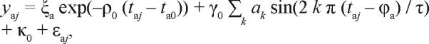
As conceptualized by Achermann and Borbély,¹⁵ performance may be modeled by assuming an additive interaction of the circadian and homeostatic processes. The general equation for this would be

5.

where P is the predicted level of performance, β is a parameter for the relative impact of the homeostatic process on performance, and γ is a parameter for the amplitude of the effect of the circadian process on performance. The intercept parameter κ offsets the 2 processes and thereby modulates the basal performance level. Substituting Eqs. (1) and (4) into Eq. (5), and noting that β is redundant with ξ (i.e., they only occur together as β ξ and may therefore be replaced by a single, rescaled parameter ξ), it follows that

6.

The free parameters in this performance model are ρ, γ, κ, ξ and ϕ There is experimental evidence that the homeostatic build-up rate ρ,^16,17 the circadian amplitude γ,^6(fn.a) and the basal performance level as determined by κ,¹⁸ depend on individual subjects' trait characteristics. These parameters will therefore be considered trait parameters.

The initial homeostatic state ξ and the circadian phase angle ϕ cannot normally be considered trait parameters; they may change for any given individual depending on the circumstances (e.g., due to recent sleep loss and/or circadian phase shifting from a bout of shift work) and are therefore state parameters. However, within a consolidated period of wakefulness, the initial homeostatic state ξ (i.e., the homeostatic state at the time of the most recent awakening t₀) is not subject to change. Thus, the initial homeostatic state is an enduring condition. Although the initial homeostatic state cannot be inferred from population-based data, its enduring quality makes it otherwise indistinguishable from a trait for the purpose of parameter estimation with the Bayesian forecasting procedure. When applying that procedure to a consolidated period of wakefulness, therefore, the parameter ξ may be treated as equivalent to a trait parameter. This important property is implied throughout this paper whenever the term initial state parameter is used.

In general, the circadian phase angle cannot be considered an enduring conditionfor many operational settings, especially those involving shift work or transmeridian travel, this would be a poor approximation of reality. However, while it is possible to deal with transitory states in the Bayesian forecasting procedure, this goes beyond the scope of the paper. The work described here is limited to those circumstances under which circadian phase angle is stable and may thus be assumed to represent an enduring condition. With this qualification, circadian phase angle is not distinguishable from a trait for the purpose of parameter estimation with the Bayesian forecasting procedure. When applying the procedure, therefore, the parameter ϕ is also an initial state parameter which may be treated as equivalent to a trait parameter.

Population Model for the Two-Process Model

As described in the introduction, the Bayesian forecasting procedure makes use of the advance characterization of inter-individual variability in the population. In the present context, the procedure depends on the advance estimation of the two-process model parameters and their between-subjects variance in a sample of n subjects drawn from the population. It will be assumed that an appropriate data set is available. For illustration purposes, such a data set will be introduced later in this paper.

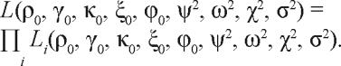
The two-process model parameters and their between-subjects variance can be estimated on the basis of the available data using the following mixed-effects regression equation:

7.

where y_ij represents the data for subjects i (i = 1, …, n) at time points t_ij (with j indexing the data points), and ε_ij stands for independent, normally distributed residual error with mean zero and variance σ². P_i is the subject-specific version of the performance model in Eq. (6):

8.

Here ρ_i, γ_i, κ_i, ξ_i and ϕ_i are the subject-specific model parameters, and t_i0 is the subject-specific modeling start time.

To estimate between-subjects variance in the trait parameters, it will be assumed a priori that ρ_i and γ_i are lognormally distributed over subjects around ρ₀ and γ₀, respectively, and that κ_i is normally distributed over subjects around κ₀. It will also be assumed that there is no covariation over subjects among ρ_i, γ_i and κ_i. The assumptions about the distribution types for these “random effects” are weak.⁹ It is not critical for the shape of the assumed distributions to describe the data very precisely, as the effect thereof on the results of the Bayesian forecasting procedure is limited. Some statistical and numerical efficiency may be gained by explicitly modeling the covariation between pairs of random effects, but that issue is beyond the scope of this paper.

The distributions of the initial state parameters ξ _i and ϕ_i depend on the conditions under which the available data were collected. Specifically, for the data set introduced in the next section, by design the initial homeostatic state ξ and the circadian phase angle ϕ should be approximately the same for all subjectssay, ξ₀ and ϕ₀, respectively. (Later in this paper, however, ξ and ϕ will be considered uncertain for simulation purposes.)

Taken together, these assumptions, or prior distributions, can be translated into the following mathematical equations:

9.

where ν_i, η_i and λ_i are independently normally distributed with means of zero and variances ψ², ω² and χ², respectively. Characterization of the trait inter-individual variability in the population in the framework of the two-process model thus entails the assessment of the normal distributions for ν_i, η_i, and λ_i by estimating the parameters ψ², ω² and χ². For reference purposes, the relevant model parameters are recapitulated in Table 1.

Table 1.

Summary Descriptions of the Trait Parameters (Distinguishing Their Fixed Effects, the Associated Subject-Specific Random Effects, and the Variances Thereof Across the Population) and Other Model Parameters (Initial State Parameters, Residual Error) Involved in the Bayesian Forecasting Procedure

Trait Parameters	Homeostatic build-up rate	ρ (fixed effect)
		ν (random effect)
		ψ2 (population variance)
	Circadian amplitude	γ (fixed effect)
		η (random effect)
		ω2 (population variance)
	Basal performance level	κ (fixed effect)
		λ (random effect)
		χ2 (population variance)
State Parameters	Initial homeostatic state	ξ (subject-specific)
	Circadian phase angle	ϕ (subject-specific)
Residual Error	Error variance	σ2 (population variance)

Substitution of Eqs. (8) and (9) into Eq. (7) leads to the following formulation of the mixed-effects regression equation:

10.

The parameters of this regression equation can be estimated by means of maximum likelihood estimation. Let the probability density function (pdf) of a normal distribution with mean m and variance s² for a variable x be denoted as p[x; m, s²]. The likelihood l_i of observing the data y_ij for a given subject i can be expressed as a function of the regression parameters, as follows:

11.

where σ² is the variance of the residual error, and c is an (irrelevant) normalization constant.

Integration over the assumed normal distributions for ν_i, η_i and λ_i to account for the relative probabilities of all possible values of these parameters yields the marginal likelihood L_i:

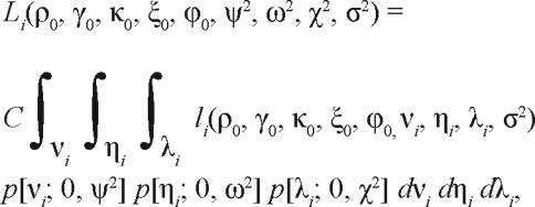12.

where the integrals each run from −∞ to ∞, and C is an (irrelevant) normalization constant. It follows that the likelihood L of observing the entire data set, for all subjects collectively, can be expressed as a function of the regression parameters, as follows:

13.

Maximum likelihood estimation entails assessment of those parameter values that would make it maximally likely for the data to be observed as they were, i.e., those parameters that maximize L. This is typically done by minimizing −2 log L, which is equivalent to maximizing L but is easier to perform numerically. The ensuing parameter estimates establish what is called the population model. Here, the population model characterizes the consistent changes in performance over time according to the two-process model, the systematic between-subjects variance (i.e., trait-like variability) in the parameters of the two-process model, and the residual within-subjects variance (i.e., error variance) in the sample representing the population.

Bayesian Forecasting with Unknown Traits and Uncertain States

Once the population model has been established, it can be used in the Bayesian forecasting procedure to optimize the parameters of the two-process model and to make subject-specific predictions of future performance for an individual not studied beforehand. Let's indicate this individual with index “a.” The subject's trait parameters are thus represented by ν_a, η_a and λ_a, and the subject's initial state parameters are ξ_a and ϕ_a. Recasting Eq. (10) yields:

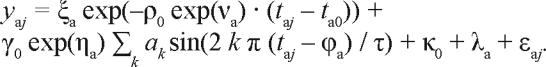14.

Fixing ρ₀, γ₀, κ₀, ψ², ω², χ² and σ² at their established population values, the subject-specific parameter optimization task focuses on estimating ν_a, η_a, λ_a, ξ_a and ϕ_a.

At first, when no performance data are as yet available for the subject, the most likely estimates for the subject's traits are those that correspond to the “average” subject in the populationi.e., ν_a = 0, η_a = 0 and λ_a = 0. Such reasoning would not normally be valid for the subject's initial homeostatic state ξ_a and circadian phase angle ϕ_a. With ν_a, η_a and λ_a fixed at zero, however, Eq. (14) would reduce to:

15.

in which only ξ_a and ϕ_a are free parameters. With 3 performance measurements for the individual at hand, first estimates for the initial state parameters ξ_a and ϕ_a can generally be obtained from this equation. This suggests that, as a rule of thumb, Bayesian forecasting estimates for the subject's model parameters may begin to be reliable when the third performance measurement becomes available (and with every measurement thereafter).

Let the probability density function (pdf) of a uniform distribution over the interval from a to b for a variable x be denoted as u[x; a, b]. Assuming that the distributions represented by the parameters ν_a, η_a, λ_a, ξ_a and ϕ_a in Eq. (14) are independent of each other and of the noise term ε_aj, maximum a posteriori estimates for the state and trait parameters are obtained by maximizing the Bayesian expression

16.

given the subject's available data y_aj (j = 1, 2, 3, …). Here, l_a is the likelihood function taken from Eq. (11) with ρ₀, γ₀, κ₀ and σ² fixed; and L_a is defined analogous to the marginal likelihood in Eq. (12):

17.

Here the integrals for ν_a, η_a and λ_a run from −∞ to ∞; and the integrals for ξ_a and ϕ_a run from −∞ to 0 and from 0 to τ, respectively.

The normal distribution factors in expression (16) represent the prior probability information about the trait parameters, as engendered in the population model. No such prior information is available for the initial state parameters, which is why they are assigned uniform distributions across the ranges of their possible values. For the purpose of maximization, the uniform distributions for ξ_a and ϕ_a cancel out; and the denominator L_a, being invariant to the free parameters (ξ_a, ϕ_a, ν_a, η_a and λ_a) also cancels out. As such, for maximization, expression (16) may be simplified to

18.

Maximization of expression (18), using all the available performance data y_aj for the subject at hand, yields the most likely estimates^a for the parameters ξ_a, ϕ_a, ν_a, η_a and λ_a. By repeating this maximization each time additional performance data become available, the parameter estimates improve with every such update, converging rapidly to those that statistically optimally represent the individual. Consequently, the accuracy of predictions for future performance, based on the updated parameter estimates, increases progressively. Due to first having characterized a sample of the population at large, this improvement in prediction accuracy for a previously unstudied individual occurs much more efficiently than would be possible if the individualized predictions were attempted without the use of population information.⁹

As an additional advantage, expression (18) allows estimation of how accurate the subject-specific parameter estimates and performance predictions actually are, via assessment of (95%) confidence intervals. How this is best approached depends on the numerical procedure used to deal with expression (18), and a detailed discussion is beyond the scope of the present paper. One approach currently implemented is described in the next section.

Numerical Implementation

A computer program was developed for the numerical maximization of expression (18) to estimate the parameters, and for the assessment of 95% confidence intervals for the parameter estimates and performance predictions. The computer program was written in Matlab version 7.0 (The MathWorks, Inc., Natick, Massachusetts), and was run under the Microsoft Windows XP operating system on a 1.7 GHz Intel Pentium desktop computer.

Expression (18) was maximized through a 5-dimensional grid search, which involved calculating the outcome across many combinations of possible parameter values and recording the largest outcome encountered. The parameter grid was made up of ν_a ranging from −3 to 3 in intervals of 0.5; η_a ranging from −2 to 2 in intervals of 0.25; λ_a ranging from −30 to 30 in intervals of 3; ξ_a ranging from −120 to 0 in intervals of 15; and ϕ_a ranging from 0 to 21 in intervals of 3 (due to the 24 h circularity of ϕ_a there was no need to evaluate ϕ_a at 24). The grid ranges for the (non-circular) parameters ν_a, η_a, λ_a and ξ_a were selected such that the probability density represented by expression (18) vanished toward the boundaries. To increase the computational efficiency, calculation of Eq. (11) as embedded in expression (18) was done recursively, and the irrelevant constant c in the formula was ignored (i.e., set to 1).

Recording the largest outcome encountered in the grid search merely resulted in crude first estimates of the parameters. To enhance the numerical resolution of the parameter estimates, the parameter grid was interpolated by a factor 4 in each dimension using piecewise cubic splines. Effectively this involved approximating the outcomes for a grid with a higher resolution by connecting all the values in the original grid with a smooth (multi-dimensional) surface. The largest outcome in the interpolated grid, found close to the original maximum, was recorded to determine the final parameter estimates. These parameter values were then entered into Eq. (14) (minus the error term ε_aj) to yield the most probable prediction of future performance (for given time t).

For each performance prediction, a 95% confidence interval was calculated by first identifying the smallest contiguous portion of the (interpolated) parameter grid that captured 95% of the total area under the curve given by expression (18). All combinations of parameter values included in this portion of the grid were then entered into Eq. (14) to compute the corresponding predictions of future performance (for given time t). The minimum and maximum of the performance predictions encountered in this process were taken as estimates of the boundaries of the 95% confidence interval (which was thereby allowed to be asymmetrical). Further work (e.g., with Monte Carlo simulations) is needed to validate these estimates.

Bayesian 95% confidence intervals for the parameter estimates proper were derived by constructing the marginal probability density functions (pdfs). These are the pdfs for every parameter considered individually while accounting for the probability densities of the other parameters. The marginal pdf for each parameter was computed by integrating over the other 4 parameters across the parameter grid. All marginal pdfs thus obtained were interpolated by a factor 30 using piecewise cubic splines. (This involved approximating the values for a grid with higher resolution by connecting all the values in the original grid with an appropriate, smooth curve.) The maxima of the interpolated marginal pdfs were identified in order to obtain more precise estimates for the individual model parameters. Lastly, 95% confidence intervals for the parameter estimates were computed by assessing the shortest contiguous interval capturing 95% of the area under the curve of each marginal pdf.¹⁹

Average prediction bias (i.e., systematic under- or over-prediction) was quantified by calculating the average difference between predictions and actual observations. Furthermore, average prediction error (i.e., point by point deviation) was quantified by computing the square root of the average squared difference between predictions and actual observations (i.e., the root mean square error).

Experimental Data and Corresponding Population Model

To illustrate the potential of the Bayesian forecasting approach, a previously established data set was employed to run simulations. The data were collected during a laboratory study involving 88 h of total sleep deprivation, as described elsewhere.²⁰ During the sleep deprivation period, a range of cognitive performance outcomes was measured every 2 h, from 07:30 until 23:30 three days later. Performance on the psychomotor vigilance test (PVT) was selected as the outcome measure to model, because of demonstrated validity and sensitivity to the homeostatic and circadian processes.²¹ The number of lapses (reaction times ≥ 500 ms) on the PVT was recorded as the primary outcome variable y.

Data from n = 10 subjects in the study, drawn from a population of healthy males aged 21 to 50 years, were used to derive a population model based on the two-process model, as per Eq. (10). Figure 1 displays the data from this sample, averaged over subjects. Performance deteriorated across days of sleep deprivation in accordance with the homeostatic process (Eq. (4)), and varied rhythmically within each day in accordance with the circadian process (Eq. (1)).²⁰ The average level of performance impairment reached after multiple days of total sleep deprivation was considerableit appeared to exceed the average level of performance impairment resulting from being legally intoxicated by alcohol.²² However, there were substantial inter-individual differences in the effects of sleep deprivation on psychomotor vigilance performance, as illustrated by the inset in Figure 1. The bar shows the interval of ±1 standard deviation for systematic between-subjects variability, as determined by mixed-effects analysis of variance.²³

Figure 1.

Performance measurements during a laboratory study involving 88 h of total sleep deprivation, and population model of performance based on the two-process model. The solid boxes show the number of lapses (reaction times ≥ 500 ms) on a psychomotor vigilance test administered every 2 h, averaged over subjects (n = 10). Upwards in the graph corresponds to greater performance impairment. The thin curve shows the population model as plotted for the “average” subject. The averaged data are captured well by this curve. However, the averaged data do not show the considerable inter-individual differences throughout the sleep deprivation period. The bar in the inset depicts the interval of ±1 standard deviation for between-subjects variability in the data. Although difficult to illustrate graphically, these inter-individual differences are captured well by the population model also.

The population model was assessed using Eqs. (9) through (13), as evaluated with the computer software NONMEM version V (GloboMax LLC, Hanover, Maryland). Time t was expressed as cumulative clock time (in hours) with time 0 defined as the midnight preceding the total sleep deprivation period. The sleep deprivation began at 07:30, and this time point was used to define the modeling start time, so that t₀ = 7.5 for all subjects. Subject selection criteria and experimental controls²⁰ standardized the initial homeostatic state ξ and circadian phase angle ϕ at the beginning of sleep deprivation. For the purposes of assessing the population model, therefore, these 2 parameters were considered the same for all 10 subjects in the sample. The circadian phase angle was relatively stable during the 88 h of total sleep deprivation,¹⁴ indicating that the initial state parameter ϕ represented an enduring condition under these circumstances.

The parameter estimates (± standard errors) for the population model were found to be as follows: ρ₀ = 0.0350 (± 0.0156), γ₀ = 4.30 (± 1.05), κ₀ = 29.7 (± 3.7), ξ₀ = −28.0 (± 4.4), ϕ₀ = 0.6 (± 0.2), ψ² = 1.15 (± 0.41), ω² = 0.294 (± 0.191), χ² = 36.2 (± 26.2), and σ² = 77.6 (± 7.3). Figure 1 shows that the population model closely matched the data as averaged over subjects. Not readily observed in Figure 1 is that the population model also matched the data of the individual subjects well, since the parameters of the population model were optimized relative to the data of the whole sample of n = 10 subjects without averaging out the considerable inter-individual differences. Compared to the same model without inter-individual differences, the population model reduced the residual error variance by a factor 1.64.

The population model described here characterized the changes in performance during total sleep deprivation in accordance with the two-process model, as well as the inter-individual differences in the model parameters and the residual error, in a population of healthy males aged 21 to 50 years. This provided all the information necessary to run simulations for the Bayesian forecasting procedure, in order to demonstrate the predictability of individual subjects' performance in the face of a priori unknown traits and uncertain states.

Bayesian Forecasting Simulations

Besides the 10 subjects used to establish the population model, 3 additional subjects drawn from the same population participated in the total sleep deprivation study described above. These 3 subjects were selected to represent considerable inter-individual differences in performance impairment during sleep deprivation, and their data were set aside prospectively to run simulations with the Bayesian forecasting procedure. The trait parameters ν_a, η_a and λ_a for these subjects were not known a priori. Furthermore, even though the initial state parameters ξ_a and ϕ_a were approximately the same for all subjects due to the design of the study,²⁰ for the purposes of simulations these parameters were considered uncertain.

The objective of the first of our simulations was to make predictions of the 3 subjects' performance during total sleep deprivation, at 1 h intervals for up to 24 h in the future (i.e., 24 h ahead predictions); and to update the predictions using Bayesian forecasting each time the next performance measurement became available. The population model parameters ρ₀, γ₀, κ₀, ψ², ω², χ² and σ² remained fixed at their previously established population averages (see the previous section). Modeling start time t_a0 was fixed at 7.5 (i.e., 07:30, the scheduled time of awakening). Time t_aj was incremented in 2 h steps beginning at t_a0, so as to coincide with the time points for data collection in the sleep deprivation experiment. At each increment, parameter estimates were updated by maximizing expression (18) using the numerical approach outlined earlier. With the updated parameter estimates, Eq. (14) (minus the error term ε_aj) was evaluated at 1 h intervals from t_aj to t_aj + 24 in order to predict performance up to a 24 h prediction horizon.

Figure 2 shows the results of the simulation, in snapshots taken at 8 h intervals. The 3 subjects are indicated as “A”, “B,” and “C.” The first snapshot (top row panels in Figure 2) occurred at 11:30, at 4 h awake, when the third performance measurement was taken. Based on the rule of thumb suggested by Eq. (15), this is the first occasion when there may have been enough data points (black circles) to reasonably estimate the initial state parameters ξ_a and ϕ_a. Even at this early stage, the 24 h predictions for the 3 subjects (solid curves) were already notably different, accounting with remarkable accuracy for the different performance profiles that would subsequently be observed in the actual measurements (gray circles). However, the 95% confidence intervals for the performance predictions were still large. The last snapshot (bottom row panels in Figure 2) was taken 40 h later, well before the end of the 88 h sleep deprivation period, but sufficiently far along for the present purposes. By this time (i.e., at 44 h awake), the 24 h predictions had diverged substantially among the 3 subjects, as had the actual observations. Also, the 95% confidence intervals for the performance predictions were much narrower. There was no overlap between the 95% confidence intervals for subjects B and C at any of the evaluated time points (at 1 h intervals) across the 24 h prediction horizon (center and right bottom panels in Figure 2). This implies that at 44 h awake, the predictions for these 2 individuals were statistically distinct, with a type I error of much less²⁴ than 0.05 for every prediction time point.

Figure 2.

Simulation using the Bayesian forecasting procedure to predict performance over time for 3 individuals exposed to acute total sleep deprivation. Each column of panels represents a different individual. Subject “A” exhibited a fairly average response to sleep deprivation (cf. Figure 1); subject “B” displayed considerable resistance to the effects of sleep deprivation; and subject “C” had relatively high vulnerability to performance impairment due to sleep deprivation. However, these subject-specific characteristics were not clear in advancein this simulation, the trait parameters ν, η and λ were assumed a priori unknown, and the initial state parameters ξ and ϕ were considered a priori uncertain as well. The first row of panels shows the performance predictions for each of the 3 individuals upon acquisition of the third performance measurement, at 4 h awake (11:30 clock time). The black circles show the number of lapses (reaction times ≥ 500 ms) on a psychomotor vigilance test administered every 2 h up to that time point. The thick curve shows the psychomotor vigilance performance predictions for the subsequent 24 h period. The thin vertical lines display the corresponding 95% confidence intervals (in 1 h steps). For comparison, the gray circles show the actual performance measurements during the 24 h prediction period. (Since this was a simulation based on data acquired previously, these observations were already known, even though they were not yet made available to the Bayesian forecasting procedure.) Note that any data points that visually seem to be missing have the prediction curve right on top of them. The second row of panels shows the situation 8 h later, when 4 additional performance measurements were available, and the model parameters had been updated accordingly by the Bayesian forecasting procedure. The third through sixth rows show the situation in further 8 h increments.

Since the sleep deprivation study took place in the past and all the data were already available, the simulation predictions could be compared directly to actual observations of performance impairment. Looking at all the snapshots in succession (from top to bottom through Figure 2), the performance responses to sleep deprivation varied systematically among the 3 individuals. The model predictions were progressively tailored to these subject-specific responses, and the 95% confidence intervals consistently reduced in size, revealing a steady increase in model precision. Of course, this does not mean that the predictions were highly accurate throughout. Occasionally, performance at specific time points was considerably under- or over-predicted. However, the observations at those time points typically stood out from the surrounding data points, and did not fit the expected profile of gradual change over time in accordance with the homeostatic and circadian processes. Whether these data points represent outliers or whether they may reflect systematic aspects of performance regulation not captured by the two-process model is difficult to establish. Ultimately, the Bayesian forecasting procedure can only predict performance as well as allowed by the comprehensiveness of the biomathematical model in which it is implemented, and the quality of the data it uses to update the model parameters. Given these caveats, the simulation demonstrated a high degree of success in predicting performance 24 h ahead during laboratory sleep deprivation.

Figure 3 shows the evolution of the model parameter estimates with every step in the simulation, from 4 h awake up to 70 h awake, for subject “A.” The figure illustrates that the 3 trait parameters as well as the 2 initial state parameters could be estimated with increasing precision as more data became available over time. However, this “sharpening up” of the parameter estimates did not always occur in a gradual fashion. Occasional abrupt changes reflected variability in how informative the newly acquired performance data were for the parameters in question. After about 50 h of wakefulness, there was hardly any new information in the performance data, and the parameters converged on their best estimable values. The estimates of the trait and initial state parameters for each of the 3 subjects at the end of the simulation, after 88 h of total sleep deprivation, are shown in Table 2. For comparison, the population averages of the trait parameters were zero by definition, and the population averages of the initial state parameters were ξ₀ = −28.0 and ϕ₀ = 0.6.

Figure 3.

Bayesian forecasting estimates of the trait and initial state parameters for subject “A”. This figure illustrates the optimization process for the estimates of trait parameters ν, η, and λ and initial state parameters ξ and ϕ during the simulation shown in Figure 2. The panels display the parameter estimates (diamonds) with 95% confidence intervals (vertical bars), as updated upon the availability of new performance measurements at 2 h intervals (beginning with the third measurement at 4 h of wakefulness). Note that even though circadian phase angle ϕ was estimated in the range from 0 to 24, it is plotted here (last panel) on a scale from −12 to 12 to facilitate visual interpretation. The confidence intervals for the first two estimates of ϕ extend below the bottom of the panel, and are continued at the top of the panel because of the circular nature of this parameter. For reference purposes, the open diamonds mark the parameter estimates that were underlying the performance predictions for subject “A” as shown successively in the 6 panels in the left column of Figure 2.

Table 2.

Estimates of the Trait and Initial State Parameters for the 3 Individual Subjects, as Converged on After 88 h of Total Sleep Deprivation in Computer Simulations Starting at Awakening

Individual	Trait Parameters			State Parameters
	ν	η	λ	ξ	ϕ
A	0.12	0.75	2.8	−44.5	0.0
B	−2.37	−0.44	−3.1	−30.0	3.3
C	0.88	−0.13	3.5	−39.5	−2.8*

^*Even though circadian phase angle ϕ was estimated in the range from 0 to 24, it is shown here on a scale from −12 to 12 to facilitate comparison among individuals.

It is instructive to assess the performance prediction accuracy of the Bayesian forecasting procedure relative to that of the population average model (i.e., with the traits and initial states fixed at the estimates obtained when establishing the population model). The latter is illustrated in Figure 4 for a snapshot taken at 44 h of wakefulness. A visual comparison of this simulation with the one in Figure 2 (last row panels) suggests that using the population average model had limited consequences for subject “A” (because this subject's response to sleep deprivation turned out to be approximately average), but resulted in substantial over-prediction of performance impairment for subject “B” and under-prediction of performance impairment for subject “C.” The average prediction bias at 44 h awake for the 3 subjects combined was −4.4 lapses, and the average prediction error was 16.3 lapses. In contrast, for the simulation with the Bayesian forecasting procedure (Figure 2), the average prediction bias at 44 h awake was only −0.2 lapses, and the average prediction error was 8.0 lapses. These numbers demonstrate the improvement achieved by using the Bayesian forecasting procedure to predict performance under conditions of unknown traits and uncertain states.

Figure 4.

Simulation using the population model based on the two-process model to predict performance over time, without employing the Bayesian forecasting procedure. Details are the same as for the last row of panels (awake 44 h) in Figure 2, except that the state and trait parameters of the performance prediction model remained fixed at their population averages and were not updated based on subject-specific performance information acquired during the sleep deprivation period. As a consequence, the performance predictions were equal for each individual, and there was no flexibility in the level or shape of the 24 h predictions curves. Note also that no suitable equivalent was available for the 95% confidence intervals.

Because the 3 subjects set aside for simulations were taken from the same study as the 10 subjects used to establish the population model, their initial homeostatic and circadian state parameters may have been relatively close to the population averages. Indeed, the parameter values at the end of the simulation (Table 2) confirmed this. To rule out that our evaluation of the Bayesian forecasting procedure under conditions of state uncertainty constituted a poor test because of this, another simulation was run similar to the first one (Figure 2), but starting at a different homeostatic state. This was accomplished by ignoring the first 24 h of sleep deprivation and the performance data collected during this period, and beginning the simulation at t_a0 = 31.5 (i.e., 07:30 of the second day of sleep deprivation). All other aspects of the simulation were kept the same.

Figure 5 shows the results of this new simulation for subject “A,” in snapshots taken at 8 h intervals. In terms of time spent awake, the top panel in Figure 5 corresponds to the fourth panel in the left column of Figure 2—both represent the situation at 28 h awake. Since the performance data acquired during the first 24 h of wakefulness were ignored in the new simulation, however, the 24 h performance predictions made at 28 h awake were slightly different, and the 95% confidence intervals were much larger. Still, over time (from top to bottom through Figure 5), the Bayesian forecasting procedure displayed the same behavior, progressively tailoring the predictions to the subject-specific responses with the 95% confidence intervals consistently reducing in size. At 44 h of wakefulness (i.e., the third snapshot), the average prediction bias across all 3 subjects was −1.5 lapses, and the average prediction error was 8.9 lapses—not much different from the first simulation (Figure 2) and still much better than the population average model simulation (Figure 4). The estimates of the trait and initial state parameters for each of the 3 subjects at the end of the simulation, after 88 h of total sleep deprivation, are shown in Table 3. By and large, these estimates are close to those obtained in the first simulation (Table 2). These results confirm that the Bayesian forecasting procedure, as extended by us from the trait-only procedure presented by Olofsen and colleagues,⁹ can handle the a priori uncertainty of initial states well.

Figure 5.

Simulation using the Bayesian forecasting procedure to predict performance over time for subject “A,” starting at a later time during the sleep deprivation period. Details are the same as for Figure 2 (left column panels), except that here the initial homeostatic state was different because the simulation was started at 24 h awake (but for the purpose of the simulation the amount of prior wakefulness was considered not known). Timewise, the top panel in this figure corresponds to the fourth panel in the left column of Figure 2. The second through sixth panels display the updated 24 h performance predictions as time passed, shown in 8 h increments. Note that there were only 9 actual observations (gray circles) to compare to in the last panel, because data acquisition stopped at 88 h awake in the laboratory experiment.

Table 3.

Estimates of the Trait and Initial State Parameters for the 3 Individual Subjects, as Converged on After 88 H of Total Sleep Deprivation in Computer Simulations Starting 24 H After Awakening.

Individual	Trait Parameters			State Parameters
	ν	η	λ	ξ	ϕ
A	0.47	0.76	0.0	−44.5	0.0
B	−2.05	−0.32	−3.9	−31.0	3.2
C	1.38	0.11	3.4	—*	−3.0

^*ξ could not be estimated from subject C's data after 24 h of wakefulness, as this parameter no longer had a noticeable effect on the subject's performance predictions.

Critical for the usefulness of the Bayesian forecasting procedure in operational settings is its ability to deal with sparse data, collected infrequently at intervals of potentially unequal duration. To examine this property, another simulation was conducted, similar again to the first one (and starting at t_a0 = 7.5), but using only the performance measurements of 8 (instead of 23) randomly selected time points to updated the model parameters. Figure 6 shows the results of this simulation for subject “A,” again in snapshots taken at 8 h intervals. In terms of time spent awake, the top panel in Figure 6 corresponds to the second panel in the left column of Figure 2—both represent the situation at 12 h awake (at 4 h awake there were not enough data points yet to expect reasonable estimates for the initial state parameters).

Figure 6.

Simulation using the Bayesian forecasting procedure to predict performance over time for subject “A,” under conditions of sparse data availability. A large portion of the original data set (see Figure 2, left column panels) was discarded here, so as to simulate that the available performance measurements occurred infrequently—at random, unequally spaced intervals. Other details are the same as for Figure 2, except that the first panel in that figure (awake 4 h) is not repeated because only one data point was available during the first 4 h of wakefulness in this simulation.

The scarcity of data in the simulation of Figure 6 caused the 24 h ahead prediction curve at 12 h awake to be notably different than in the first simulation (Figure 2). The 95% confidence intervals were larger as well. However, as the simulation progressed (from top to bottom through Figure 6), the 24 h predictions became very similar to those seen in the first simulation. At 44 h awake, the average prediction bias across all 3 subjects was –0.5 lapses, and the average prediction error was 8.5 lapses—again similar to what was found in the first simulation (Figure 2). The estimates of the trait and initial state parameters for each of the 3 subjects at the end of the simulation, after 88 h of total sleep deprivation, are shown in Table 4. These are also close to the estimates obtained in the first simulation (Table 2). Thus, the main effect of the data being sparse appeared to be that the 95% confidence intervals reduced in size less rapidly, but the Bayesian forecasting procedure did not lose its ability to predict.

Table 4.

Estimates of the Trait and Initial State Parameters for the 3 Individual Subjects, as Converged on After 88 H of Total Sleep Deprivation in Computer Simulations with Sparse Data.

Individual	Trait Parameters			State Parameters
	ν	η	λ	ξ	ϕ
A	0.48	0.58	2.6	−48.0	0.0
B	−1.97	−0.25	−4.1	−30.5	5.6
C	0.35	−0.17	0.4	−26.0	2.6

Repeated Use of Bayesian Forecasting

After the Bayesian forecasting procedure has been applied to make performance predictions for a given individual, the optimized values for the trait parameters (but not the initial state parameters) can be used again if predictions are needed for this same individual on another occasion. Specifically, the prior normal distributions for the trait parameters ν_i, η_i and λ_i in Eq. (18) can be replaced by the pdfs obtained for these parameters at the end of the previous application of the Bayesian forecasting procedure. This way, the data acquired for an individual during scenarios in the past continue to contribute to the precision of the performance predictions for that individual in the future.

To examine this idea, a simulation was run using data from a different experiment (study 2 in Van Dongen et al²⁵). A person was exposed to 36 h total sleep deprivation in the laboratory on 2 occasions. Laboratory circumstances were similar to those encountered in the other simulations. However, the 36 h sleep deprivations began at 10:00, and this time point was used to define the modeling start time for each sleep deprivation period (i.e., t₀ = 10). Psychomotor vigilance testing occurred at 2 h intervals, beginning at 10:30 (t = 10.5) during both sleep deprivations. The performance data were very similar between the 2 sleep deprivations (see Figure 7), as was anticipated given that performance responses to sleep deprivation are overall trait-like.⁶ It was expected that, despite the relatively small number of data points available, the Bayesian forecasting procedure would achieve greater prediction precision more rapidly for the second exposure to sleep deprivation when utilizing the trait information obtained in the first exposure.

Figure 7.

Simulation using the Bayesian forecasting procedure to predict performance over time for a single individual exposed to acute total sleep deprivation twice. The first column of panels shows the simulation for the first time the individual underwent 36 h sleep deprivation; graphical details are the same as for Figure 2. (Note that the 24 h ahead predictions displayed in the bottom panel extend beyond the 36 h period of sleep deprivation.) The second column of panels shows the simulation for the second time the individual was exposed to 36 h sleep deprivation, retaining no information from the first exposure. The third column of panels shows the simulation for the second exposure to sleep deprivation again, but—as denoted by the asterisk—the estimates for the trait parameters at the end of the first exposure to 36 h sleep deprivation were used as prior information this time (although the initial state parameters were still considered a priori uncertain).

The results of the simulation are shown in Figure 7. The first column of panels shows the results of Bayesian forecasting for the first sleep deprivation period. The second column of panels shows the results for the second sleep deprivation period without utilizing the trait information acquired in the first. Although some data points were missing in the first sleep deprivation session, the prediction results and corresponding 95% confidence intervals were nearly identical. The average prediction bias was −4.3 lapses for the first, and −6.0 lapses for the second sleep deprivation; and the average prediction error was 11.2 lapses for the first, and 11.0 lapses for the second sleep deprivation. The third column of panels shows the improvement in the predictions for the second sleep deprivation when employing the pdfs obtained for the trait parameters (but not the initial state parameters) at the end of the first sleep deprivation. Using these pdfs as prior information, the average prediction bias for the second sleep deprivation was reduced to 0.5 lapses, and the average prediction error was reduced to 6.9 lapses.

The improvement stemmed from the fact that the trait and initial state parameters converged more rapidly to the values best characterizing the individual at hand, due to the more informative prior distributions for the trait parameters. As a result, the performance predictions became more accurate, and the 95% confidence intervals were consistently smaller, than without the use of the information from the first exposure to sleep deprivation (compare the second and third columns in Figure 7). This illustrates that the Bayesian forecasting procedure can become more effective when used repeatedly.

DISCUSSION

This paper demonstrated the usefulness of the Bayesian forecasting procedure for predicting cognitive performance impairment with a biomathematical model, in particular the two-process model, in the face of unknown trait characteristics and uncertain initial states in individual subjects. Prospective computer simulations were run using data from the psychomotor vigilance test (PVT), a marker of changes in cognitive performance mediated by the homeostatic and circadian processes,²¹ as recorded during a laboratory-based study of total sleep deprivation. The simulations showed that biomathematical model parameters converged rapidly to the values that best characterized the individuals concerned, resulting in substantially improved performance predictions relative to the original version of the model. The Bayesian forecasting procedure also estimated 95% confidence intervals for the parameter estimates and for performance prediction accuracy. Over time, the 95% confidence intervals for performance shrunk, both in absolute size and relative to the differences in performance predictions among individuals, resulting in statistically relevant differentiation among subjects—i.e., successfully individualized performance predictions. Numerical computations were sufficiently fast on a Pentium-driven desktop computer to be feasible in real time in operational environments (even for keeping track of multiple individuals working in small teams).^b Thus, the work presented here provides the first solution to some of the most significant challenges in the development of biomathematical models of performance for operational use^4,5:

• performance prediction for individuals (instead of groups) in the face of a priori unknown trait inter-individual variability;

• performance prediction for individuals in the face of uncertain initial states;

• quantification of prediction accuracy.

The Bayesian forecasting procedure as implemented in the two-process model possesses broad generalizability, in that it can be used to predict waking performance in any scenario and in any population for which the two-process model proper is valid. Thus, the procedure should work in total sleep deprivation, acute sleep restriction, acute sleep displacement, and nap sleep scenarios.²⁶ Furthermore, besides healthy adults, it may work in other populations such as adolescents,²⁷ people with depression,²⁸ and patients with seasonal affective disorder.²⁹ Although it is important to establish a population model for the target population, it is not necessary to assess the population model under the same circumstances as those for which the Bayesian forecasting will be used. For example, a population model established in a nap sleep scenario should be usable as a basis for Bayesian forecasting in a sleep displacement scenario. The total sleep deprivation scenario considered in this paper does not yet offer full generalizability, though, because the data set does not allow estimation of the rate of dissipation for the homeostatic process during sleep (which could be overcome by including performance data from the recovery days following sleep deprivation²⁰). Otherwise, the versatility of the Bayesian forecasting procedure is not bounded by the circumstances associated with the population model, as long as the procedure is applied in accordance with the scope of the underlying biomathematical model, and the individuals for which performance is being predicted are part of the same population as the sample that yielded the population model.

The validity of the two-process model as used to predict performance is limited, primarily, to short-term scenarios with acute sleep-related interventions. While this covers a wide range of operationally relevant scenarios, several common situations are outside the scope of the two-process model, such as chronic sleep restriction,³⁰ circadian phase shifting,³¹ and use of pharmacological fatigue countermeasures.³² The effect of sleep inertia on cognitive performance immediately after awakening³³ is also not captured by the two-process model. Various adjustments have been considered to overcome these limitations.^15,34,35 Furthermore, other models have been developed to push the envelope on performance prediction.² The Bayesian forecasting procedure may be implemented in the framework of such alternative models as well, following the same general approach as laid out in this paper. Most current biomathematical models of performance have more parameters than the two-process model, however, which may increase the number of performance measurements needed to obtain reliable subject-specific parameter estimates and may also increase the size of the 95% confidence intervals. Even so, with Bayesian forecasting, any available performance model may be utilized to make performance predictions for individuals in the face of unknown traits and uncertain states.

This paper builds on the recent work by Olofsen and colleagues,⁹ in which Bayesian forecasting was already applied to optimize subject-specific trait parameters. The present work extends this effort by for the first time including initial state parameters in the parameter optimization process. Initial state parameters can be treated as trait parameters in the context of Bayesian forecasting if they represent enduring conditions (i.e., if their values may be assumed stable over the time period for which predictions are made). However, for initial state parameters, unlike trait parameters, the optimization process does not benefit from prior information contained in the population model. Moreover, if predictions are needed for individuals who were subjected to Bayesian forecasting before, then the previously optimized values of the individuals' trait parameters may be reused to obtain more accurate predictions with fewer data points (see Figure 7)—but this Bayesian property does not transfer to the initial state parameters. Improved prior information about the initial state parameters may be acquired by other means, though. For instance, actigraphy could be used to track sleep history, and could yield probability estimates for the initial homeostatic state ξ in lieu of the assumed uniform distribution in expression (16).

The assumption of enduring initial states implies that the use of the Bayesian forecasting procedure described here is restricted to scenarios in which there are no unexpected changes in initial states—no homeostatic discontinuities (e.g., due to unreported naps) and no circadian phase shifts (e.g., due to exposure to bright light). Considerable work has been done to derive equations for the modeling of circadian phase changes (and even temporary deviations from the limit cycle process determining circadian amplitude).³⁶ Incorporation of such equations may allow substitution of the initial state parameter for circadian phase angle by a few trait parameters, thereby lifting the assumption of enduring circadian phase angle in the present work. Other approaches to maintaining performance prediction accuracy under conditions involving dynamic circadian phase changes can be envisioned as well. One such approach could entail the development of procedures relying on on-line measurements for estimating circadian phase. Current efforts, based in part on earlier work by our group,³⁷ focus on expanding the Bayesian performance prediction framework that way.

Implementation of the Bayesian forecasting procedure does not preclude performance prediction in the absence of any subject-specific data, but the underlying (group-average) biomathematical model is only outperformed when at least a few performance measurements are available for the individual at hand. However, in operational environments, it may not be possible or practical to interrupt the ongoing tasks in order to administer performance tests. Automatically measured embedded performance measures, such as lane deviation to track driver performance,³⁸ may offer a solution to this problem. An additional advantage of using embedded performance measures is that they may be directly relevant to the demands of the operational setting. Note that the same performance measure should be used for assessing the population model as for applying the Bayesian forecasting procedure. This is important because inter-individual differences in vulnerability to sleep loss appear to be dependent on the type of performance being measured.⁶

Although there is no need to know the origin of the inter-individual differences in responses to sleep loss when applying the Bayesian forecasting procedure, the accuracy of predictions may be further improved by inclusion of relevant covariates like a subject's age.⁹ As such, research aiming to identify easily measurable biomarkers of inter-individual differences in performance impairment from sleep loss should be a priority.⁷ Even so, the Bayesian forecasting procedure presented in this paper is powerful and robust enough to be considered for validation in selected operational settings. It is important to establish population models for such settings first—the distribution of the trait parameters may be different depending on the population involved, and the error variance (i.e., the estimate for σ²) may vary from one setting to another as well. Once proven effective in the field, the Bayesian forecasting procedure can be a key component of a reliable and efficient sleep/wake-based fatigue risk management tool—predicting cognitive performance impairment, and possibly even accident risk,³⁹ at the level of individuals. The implications for productivity, safety and well-being, and ultimately for the economy and for society at large,⁴⁰ could be extensive.

FOOTNOTES

1. This estimation process is closely related to maximum likelihood estimation, which is the generally preferred framework in the context of Bayesian statistics.¹⁹ It is also possible, but technically more difficult, to derive a Bayesian forecasting algorithm based on least squares estimation. Under conditions of independent, normally distributed residual error, the resulting parameter estimates should be the same.

2. For the specified grid size and interpolation factors, each prediction step took less than one minute to compute. With more sophisticated maximization algorithms and other numerical refinements, it should be possible to reduce the computation time to mere seconds per prediction step on present-day standard desktop computers.

REFERENCES

- 1.Neri DF. Preface: Fatigue and Performance Modeling Workshop, June 13–14, 2002. Aviat Space Environ Med. 2004;75:A1–A3. [PubMed] [Google Scholar]
- 2.Mallis MM, Mejdal S, Nguyen TT, Dinges DF. Summary of the key features of seven biomathematical models of human fatigue and performance. Aviat Space Environ Med. 2004;75:A4–A14. [PubMed] [Google Scholar]
- 3.Van Dongen HPA. Comparison of mathematical model predictions to experimental data of fatigue and performance. Aviat Space Environ Med. 2004;75:A15–A36. [PubMed] [Google Scholar]
- 4.Dinges DF. Critical research issues in development of biomathematical models of fatigue and performance. Aviat Space Environ Med. 2004;75:A181–A191. [PubMed] [Google Scholar]
- 5.Friedl KE, Mallis MM, Ahlers ST, Popkin SM, Larkin W. Research requirements for operational decision-making using models of fatigue and performance. Aviat Space Environ Med. 2004;75:A192–A199. [PubMed] [Google Scholar]
- 6.Van Dongen HPA, Baynard MD, Maislin G, Dinges DF. Systematic interindividual differences in neurobehavioral impairment from sleep loss: Evidence of trait-like differential vulnerability. Sleep. 2004;27:423–433. [PubMed] [Google Scholar]
- 7.Van Dongen HPA, Vitellaro KM, Dinges DF. Individual differences in adult human sleep and wakefulness: Leitmotif for a research agenda. Sleep. 2005;28:479–496. doi: 10.1093/sleep/28.4.479. [DOI] [PubMed] [Google Scholar]
- 8.Dinges DF, Achermann P. Future considerations for models of human neurobehavioral function. J Biol Rhythms. 1999;14:598–601. doi: 10.1177/074873099129000939. [DOI] [PubMed] [Google Scholar]
- 9.Olofsen E, Dinges DF, Van Dongen HPA. Nonlinear mixed-effects modeling: Individualization and prediction. Aviat Space Environ Med. 2004;75:A134–A140. [PubMed] [Google Scholar]
- 10.Vonesh EF, Chinchilli VM. New York: Marcel Dekker; 1997. Linear and nonlinear models for the analysis of repeated measurements. [Google Scholar]
- 11.Van Dongen HPA, Maislin G, Dinges DF. Dealing with inter-individual differences in the temporal dynamics of fatigue and performance: importance and techniques. Aviat Space Environ Med. 2004;75:A147–A154. [PubMed] [Google Scholar]
- 12.Borbély AA. A two process model of sleep regulation. Human Neurobiol. 1982;1:195–204. [PubMed] [Google Scholar]
- 13.Borbély AA, Achermann P. Sleep homeostasis and models of sleep regulation. J Biol Rhythms. 1999;14:557–568. doi: 10.1177/074873099129000894. [DOI] [PubMed] [Google Scholar]
- 14.Van Dongen HPA, Mullington JM, Dinges DF. Circadian phase delay during 88-hour sleep deprivation in dim light: Differences among body temperature, plasma melatonin and plasma cortisol. In: Beersma DGM, Van Bemmel AL, Folgering H, Hofman WF, Ruigt GSF, editors. Sleep-wake research in the Netherlands. vol. 8. Leiden: Dutch Society for Sleep-Wake Research; 1998. pp. 33–36. [Google Scholar]
- 15.Achermann P, Borbély AA. Simulation of daytime vigilance by the additive interaction of a homeostatic and a circadian process. Biol Cybern. 1994;71:115–121. doi: 10.1007/BF00197314. [DOI] [PubMed] [Google Scholar]
- 16.Finelli LA, Baumann H, Borbély AA, Achermann P. Dual electroencephalogram markers of human sleep homeostasis: Correlation between theta activity in waking and slow-wave activity in sleep. Neurosci. 2000;101:523–529. doi: 10.1016/s0306-4522(00)00409-7. [DOI] [PubMed] [Google Scholar]
- 17.Aeschbach D, Postolache TT, Sher L, Matthews JR, Jackson MA, Wehr TA. Evidence from the waking electroencephalogram that short sleepers live under higher homeostatic sleep pressure than long sleepers. Neurosci. 2001;102:493–502. doi: 10.1016/s0306-4522(00)00518-2. [DOI] [PubMed] [Google Scholar]
- 18.Kane MJ, Engle RW. The role of prefrontal cortex in working-memory capacity, executive attention, and general fluid intelligence: An individual-differences perspective. Psychon Bull Rev. 2002;9:637–671. doi: 10.3758/bf03196323. [DOI] [PubMed] [Google Scholar]
- 19.Sivia DS. Data analysis: a Bayesian tutorial. Oxford: Oxford University Press; 1996. [Google Scholar]
- 20.Van Dongen HPA, Dinges DF. Sleep, circadian rhythms, and psychomotor vigilance. Clin Sports Med. 2005;24:237–249. doi: 10.1016/j.csm.2004.12.007. [DOI] [PubMed] [Google Scholar]
- 21.Dorrian J, Rogers NL, Dinges DF. Psychomotor vigilance performance: neurocognitive assay sensitive to sleep loss. In: Kushida CA, editor. Sleep deprivation. Clinical issues, pharmacology, and sleep loss effects. New York: Marcel Dekker; 2005. pp. 39–70. [Google Scholar]
- 22.Dawson D, Reid K. Fatigue, alcohol and performance impairment. Nature. 1997;388:235. doi: 10.1038/40775. [DOI] [PubMed] [Google Scholar]
- 23.Van Dongen HPA, Olofsen E, Dinges DF, Maislin G. Mixed-model regression analysis and dealing with interindividual differences. Meth Enzymol. 2004;384:139–171. doi: 10.1016/S0076-6879(04)84010-2. [DOI] [PubMed] [Google Scholar]
- 24.Payton ME, Greenstone MH, Schenker N. Overlapping confidence intervals or standard error intervals: What do they mean in terms of statistical significance? J Insect Sci. 2003;3:34. doi: 10.1093/jis/3.1.34. [DOI] [PMC free article] [PubMed] [Google Scholar]
- 25.Van Dongen HPA, Stakofsky AB, Baynard MD, Dinges DF. Comparison of individual differences in neurobehavioral impairment from sleep loss between two independent samples. Sleep. 2005;28:A133. [Google Scholar]
- 26.Achermann P. The two-process model of sleep regulation revisited. Aviat Space Environ Med. 2004;75:A37–A43. [PubMed] [Google Scholar]
- 27.Carskadon MA, Acebo C, Jenni OG. Regulation of adolescent sleep. Implications for behavior. Ann NY Acad Sci. 2004;1021:276–291. doi: 10.1196/annals.1308.032. [DOI] [PubMed] [Google Scholar]
- 28.Borbély AA. The S-deficiency hypothesis of depression and the two-process model of sleep regulation. Pharmacopsychiatry. 1987;20:23–29. doi: 10.1055/s-2007-1017069. [DOI] [PubMed] [Google Scholar]
- 29.Koorengevel KM, Beersma DGM, Den Boer JA, Van den Hoofdakker RH. Sleep in seasonal affective disorder patients in forced desynchrony: an explorative study. J Sleep Res. 2002;11:347–356. doi: 10.1046/j.1365-2869.2002.00319.x. [DOI] [PubMed] [Google Scholar]
- 30.Van Dongen HPA, Maislin G, Mullington JM, Dinges DF. The cumulative cost of additional wakefulness: Dose-response effects on neurobehavioral functions and sleep physiology from chronic sleep restriction and total sleep deprivation. Sleep. 2003;26:117–128. doi: 10.1093/sleep/26.2.117. [DOI] [PubMed] [Google Scholar]
- 31.Folkard S, Åkerstedt T, Macdonald I, Tucker P, Spencer MB. Beyond the three-process model of alertness: Estimating phase, time on shift, and successive night effects. J Biol Rhythms. 1999;14:577–587. doi: 10.1177/074873099129000911. [DOI] [PubMed] [Google Scholar]
- 32.Balkin TJ, Kamimori GH, Redmond DP, Vigneulle RM, Thorne DR, Belenky G, Wesensten NJ. On the importance of countermeasures in sleep and performance models. Aviat Space Environ Med. 2004;75:A155–A157. [PubMed] [Google Scholar]
- 33.Dinges DF, Orne EC, Evans FJ, Orne MT. Performance after naps in sleep-conducive and alerting environments. In: Johnson LC, Tepas DI, Colquhoun WP, Colligan MJ, editors. Biological rhythms, sleep and shift work. New York: SP Medical & Scientific Books; 1981. pp. 539–552. [Google Scholar]
- 34.Åkerstedt T, Folkard S. The three-process model of alertness and its extension to performance, sleep latency, and sleep length. Chronobiol Int. 1997;14:115–123. doi: 10.3109/07420529709001149. [DOI] [PubMed] [Google Scholar]
- 35.Avinash D, Crudele CP, Amin DD, Robinson BM, Dinges DF, Van Dongen HPA. Parameter estimation for a biomathematical model of psychomotor vigilance performance under laboratory conditions of chronic sleep restriction. In: Ruigt GSF, Van Bemmel AL, DeBoer T, Hofman WF, Van Luijtelaar G, editors. Sleep-wake research in the Netherlands. vol. 16. Leiden: Dutch Society for Sleep-Wake Research; 2005. pp. 39–42. [Google Scholar]
- 36.Kronauer RE, Jewett ME, Czeisler CA. Modeling human circadian phase and amplitude resetting. In: Touitou Y, editor. Biological clocks. Mechanisms and applications. Amsterdam: Elsevier Science; 1998. pp. 63–72. [Google Scholar]
- 37.Mott C, Mollicone D, Van Wollen M, Huzmezan M. Modifying the human circadian pacemaker using model based predictive control. Proceedings of the 2003 American Control Conference; 2003. pp. 453–458. [Google Scholar]
- 38.Gillberg M, Kecklund G, Åkerstedt T. Sleepiness and performance of professional drivers in a truck simulatorcomparisons between day and night driving. J Sleep Res. 1996;5:12–15. doi: 10.1046/j.1365-2869.1996.00013.x. [DOI] [PubMed] [Google Scholar]
- 39.Ingre M, Åkerstedt T, Peters B, Anund A, Kecklund G, Pickles A. Subjective sleepiness and accident risk avoiding the ecological fallacy. J Sleep Res. 2006;15:142–148. doi: 10.1111/j.1365-2869.2006.00517.x. [DOI] [PubMed] [Google Scholar]
- 40.Rosekind MR. Underestimating the societal costs of impaired alertness: safety, health and productivity risks. Sleep Med. 2005;6:S21–S25. doi: 10.1016/s1389-9457(05)80005-x. [DOI] [PubMed] [Google Scholar]