Multivariate Analysis Strategies for Processing ToF-SIMS Images of Biomaterials

Abstract

Time-of-flight secondary ion mass spectrometry (ToF-SIMS) is a hyperspectral imaging technique. Each pixel in a two-dimensional ToF-SIMS image (or each voxel in a three-dimensional ToF-SIMS image) contains a full mass spectrum. Thus, multivariate analysis methods are being increasingly used to process biomaterial ToF-SIMS images so the maximum amount of information can be extracted from the images. This study examines the use of principal component analysis (PCA) and maximum autocorrelation factors (MAF) on four different ToF-SIMS images. These images were selected because they represent significant challenges for biomedical ToF-SIMS image processing (topographical features, low count rates, surface contaminants, etc.). With PCA four different types of scaling methods (auto, root mean, filter, and shift variance scaling) were used. The effect of two preprocessing methods (normalization and mean centering) was also examined for both PCA and MAF. The more computational intense MAF provided the best results for all the images investigated in this study, doing the best job of reducing the number of variables required to describe the image, enhancing image contrast and recovering key spectral features. MAF was particularly good at identifying subtle features that were often lost in PCA and impossible to visualize in single peak images. However, the combination of PCA with either root mean or shift variance scaling provided similar results to MAF. Thus, these combinations offer promising alternatives to MAF for working with large data sets encountered in three-dimensional imaging. Also, the new method of filter scaling is promising for processing low count rate images with salt and pepper noise. Normalization proved an important tool for deconvoluting chemical effects from topographic and/or matrix effects. Mean centering aided in reducing the dimensionality of the data, but in one case resulted in a loss of information.

1. Introduction

Imaging Time-of-Flight Secondary-Ion Mass Spectrometry (ToF-SIMS) is becoming an increasingly important technique for the analysis of biomaterials and biological samples ^1–5. The rise of micro-patterned surfaces for use in biomaterials and biosensor applications has lead to a demand for analytical techniques with surface sensitivity, chemical specificity, and high spatial resolution. ToF-SIMS is one of the few techniques that offer all of these features ⁴. ToF-SIMS is a hyperspectral imaging technique. Every image pixel consists of a complete mass spectrum, with each spectrum typically containing hundreds of ion peaks. It is this hyperspectral quality which makes ToF-SIMS such an information rich technique, but it also presents substantial challenges with data handling and interpretation ⁶. With the recent development of cluster ion ToF-SIMS methods for generating 3-D image profiles the challenges for imaging processing will become even more complex ^7–9.

Although ToF-SIMS images contain a large array of data related to the identity and distribution of chemical species on a surface, processing these ToF-SIMS images to obtain concise chemical information can be a formidable challenge ^10,11. Identifying compounds and distinguishing between surface chemistry, matrix effects and topographical features typically requires simultaneous analysis of multiple ion images. As a result multivariate statistical methods have proven to be extremely valuable aids for the interpretation of ToF-SIMS images ^12–17. Although a wide variety of multivariate techniques have been applied to ToF-SIMS images, including principal components analysis (PCA), multivariate curve resolution (MCR), maximum autocorrelation factors (MAF), neural networks (NN) and mixture models (MM), PCA continues to be the most widely applied method because of its established history and wide availability ¹⁸.

PCA is designed to reduce the size of large data sets with a minimal loss of information. To do this, combinations of the original variables are identified that account for more of the variation in the total data set than any of the individual original variables. These combinations become the new variables or principal components. This process reduces the dimensionality of the data set and aids in identifying how the original variables are correlated. This has several advantages for the analysis of ToF-SIMS images. Not only does it reduce the amount of data the analyst must interpret from hundreds of individual ion images to a few principal component images, it also improves the image contrast, simplifies chemical interpretation by identifying peaks which likely arise from the same chemical species and can often help deconvolute matrix effects and topographic effects from differences in surface chemistry.

Unfortunately, the results of PCA are very sensitive to the type of pre-processing done to the data prior to PCA. In ToF-SIMS, important high mass secondary ions arising from intact or nearly intact molecules can be orders of magnitude less intense than the less specific lower mass secondary ions. Unless the data is appropriately scaled, information from these important, but low intensity secondary ions, can be buried and lost in PCA. In contrast, some other multivariate methods, including MAF and NN, are independent of scaling. In this paper, PCA, with four different scaling methods, and MAF are compared based on their ability to reduce the number of images needed to represent a data set, as well as their ability to enhance image contrast and simplify chemical interpretation.

2. Theory

A ToF-SIMS image, of dimension n-by-m pixels, can be considered as a stack of images for individual peaks within the spectra. If the spectrum contains p discrete peaks, the SIMS image will be an n-by-m-by-p array of data. For image analysis, this data array is typically rearranged into a matrix, X, where each row in the matrix contains the spectrum for an individual pixel and each column in the matrix contains an ion image for an individual peak.

2.1 Factor Analysis

PCA and MAF are both variants of factor analysis ^19–21. The goals of any type of factor analysis are 1) to reduce the number of variables needed to represent a multi-dimensional data set while minimizing the loss of information, 2) to identify relationships between variables, and 3) to identify relationships between samples. In the case of ToF-SIMS image analysis, the ion peak areas will be considered as variables and the image pixels as samples.

Factor analysis is based on the assumption that the data matrix, X, consists of k underlying component “spectra” and that each sample (or pixel) in X consists of a weighted sum of these underlying “spectra” plus random error, as shown in equation 1.

$$X=S{F}^T+E$$ (1)

where S is a matrix containing the weighting factors for each component at each pixel, F is a matrix containing the “spectra” for each component and E is a matrix containing the residual error. In ToF-SIMS imaging, the S values can be interpreted as a pseudo-concentration of an underlying component at each pixel and displayed as an image of that component. The rows of F can be interpreted as “spectra” for the underlying components.

Unfortunately, there is a rotational ambiguity, the result of which is that there are an infinite number of solutions to equation 1. PCA and MAF are both methods for calculating a desirable solution.

In PCA, the data matrix, X, is decomposed such that

$$S=XU$$ (2)

where U is the loadings matrix and S is the scores matrix. The loadings matrix, U, can be obtained via an eigenvector rotation of the matrix X^TX ^22,23. The eigenvectors in matrix U that have the largest eigenvalues will identify linear combinations of the secondary ion peaks that capture the maximum variation in the image. The first k columns of the matrix S form a solution to equation 1, where U⁻¹ = F. If X^TX is full rank, then U and F will be full rank square matrices. For typical ToF-SIMS images the number of pixels is usually much larger than the number of peaks, so X^TX will be full rank unless the data has been normalized to the sum of selected peaks. If X^TX is not full rank, then U will not be a square matrix. However, the F matrix can still be calculated from a given set of scores using a least squares procedure. Because U contains the eigenvectors of a symmetric matrix, it has the unusual property that U⁻¹ = U^T, so the loadings matrix can be directly interpreted as spectra associated with each scores image.

In MAF the data matrix X is decomposed as described in equation 2. However, the loadings matrix, U, is obtained by an eigenvector rotation of the matrix B,

$$B=A^{-1}{X}^{T}X$$ (3)

where A is the covariance matrix of the shift images. The shift images are obtained by subtracting the X matrix from a copy of itself that has been shifted by one pixel horizontally or one pixel vertically. To calculate the matrix B the covariance matrix of the shift images must be full rank. If the data have been normalized to the sum of selected peaks, this will not be the case and one of the peaks must be omitted from the analysis to obtain a real solution. The eigenvectors of matrix B that have the largest eigenvalues will identify linear combinations of secondary ion peaks which maximize the variation across the entire image while minimizing the variation between neighboring pixels ²¹. As with PCA, the scores can be displayed and interpreted as an image for an underlying component. The B matrix, however, is not symmetric, so U⁻¹ ≠ U^T. U⁻¹ is however still a solution for F in equation 1, so once the loadings are inverted, they can also be interpreted as “spectra” for underlying components.

2.2 Scaling

It is widely recognized that the effectiveness of PCA in separating valuable information from noise is dependent on appropriate image scaling. There is a growing consensus within the chemometrics community that data should be scaled based on the measurement uncertainty in the variables. In this paper, we compare four different scaling methods, each of which makes an attempt at estimating the measurement uncertainty for each peak based on the ToF-SIMS image data. The four scaling methods are auto-scaling, root mean scaling (also called optimal scaling¹³), filter scaling, and shift variance scaling.

Auto-scaling consists of dividing each peak by the standard deviation of that peak over the image. Root mean scaling consists of dividing each peak by the square root of the mean value for that peak. Filter scaling is a new method that consists of dividing each peak by the standard deviation for a restricted set of pixels near that peak. This modified standard deviation is calculated by excluding pixels that have both zero counts and no non-zero neighbors. By defining a neighborhood, such as a 3 × 3 neighborhood, the increase in variance of randomly scattered noise in isolated pixels can be limited (i.e., 9 for a 3 × 3 neighborhood). Filter scaling also maintains the order of the relative variance among the mass peaks while increasing the amount of variance in the low intensity peaks. Further details of filter scaling are described elsewhere ²⁴. Shift variance scaling is based on the same concept as MAF. The shift matrix is calculated by subtracting the X matrix from a copy of itself that has been shifted by one pixel horizontally and/or one pixel vertically. Shift variance scaling consists of dividing each peak by its standard deviation in the shift matrix.

Unlike PCA, MAF is a scaling independent technique because scaling factors applied to each peak will cancel out when the B matrix is calculated (equation 3). Identical loadings vectors are calculated regardless of any pre-scaling of the data. As a result, the different scaling methods will be explored only for PCA.

2.3 Data Pre-processing

In addition to scaling, various pre-processing techniques are commonly applied to images prior to multivariate analysis. The most common of these are normalization and mean centering. Normalization consists of dividing the spectra at each pixel by the total ion counts at that pixel. Normalization is typically done to reduce interference from topographic or matrix effects. Mean centering consists of subtracting the image mean for each peak from the image for that peak. Mean centering is typically done so the differences in the peak area variances are emphasized over differences in the peak area means.

2.4 Image Contrast

For the purposes of this paper, contrast between two regions in an image is represented by c_1,2 and is defined by equation 4 as

$$c_{1,2}=\frac{|I_1-I_2|}{{\sigma }_{1,2}}$$ (4)

where I₁ is the average intensity in region 1, I₂ is the average intensity in region 2 and σ_1,2 is the pooled standard deviation of the intensity within the two regions. The relevant value for c_1,2 is the threshold at which the boundaries between the two regions can be clearly seen with the human eye. Precise values of the threshold are subjective and will vary from viewer to viewer. For large features, this threshold is surprisingly low (<1). For 4x4 pixel features, the threshold occurs at c ≈ 2. For 2x2 pixel features, the threshold occurs at c ≈ 4. Note that the image contrast can be increased by either increasing the average difference between the two regions or decreasing the standard deviation within the regions.

3 Methods

3.1 Sample Preparation and Image Collection

Four different ToF-SIMS images were explored for this study. These images were selected because they represented challenging samples (low counts, matrix effects, topographic effects, etc.) to image process, not because they represented images fabricated or analyzed under optimal conditions. Image 1 was selected to test the ability to extract chemical information from a few small particles on a uniform background with intense signals. Image 2 was selected to test the ability to extract chemical information from low-count images with significant matrix effects. Image 3 was selected to test the ability to extract chemical information in the presence of significant topography. Image 4 was selected to extract chemical information from high-count images with significant matrix effects and surface contaminants. A description of the samples used for each image is given in the following paragraphs.

3.1.1 Image 1

The sample used to acquire Image 1 was comprised of ambient atmospheric aerosol particles on a 1 mm pore size Teflon filter. The particles were collected in Bozeman, MT, using a total suspended particulate filter sampler. The image was collected on a TRIFT II spectrometer using a 25 keV gallium ion source. A 250 μm × 250 μm area was imaged using a 256 × 256 pixel random raster. Mass resolution for the image is ~ 1500 m/Δm, which allowed the separation of elemental and organic ions. The data matrix was created by integration of 190 peaks from the raw data image.

3.1.2 Image 2

The sample used to acquire Image 2 was prepared by e-beam lithography (EBL) followed by gold deposition and chemical modification. First a thin layer of poly(methyl methacrylate) (PMMA) was spin coated onto a cleaned silicon wafer. Then EBL was used to write a series of 5 micron long lines into the PMMA. The width of the lines ranged from 50 nm to 10 microns and spacing between lines was 5 microns. After developing the pattern with methylisobutylketone, 5 nm of chromium followed by 40 nm of gold was deposited onto the substrate by thermal evaporation. Then acetone was used to strip the remaining PMMA off the surface. The chemical modification followed the approaches of Veiseh et al. and Michel et al. for selective chemical adsorption ^25–27. First a dodecanethiol self assembled monolayer (SAM) (1mM, in ethanol) was formed on the gold regions. Then poly(L-lysine)-graft-poly(ethylene glycol) (PLL-g-PEG) from a 1mg/ml solution in phosphate buffered saline (PBS) was selectively adsorbed onto the silicon regions. The dodecanethiol SAM forms a hydrophobic surface that will adsorb protein, while the PLL-g-PEG creates a non-fouling surface ^27–29. The patterned chip was then immersed in a 100μg/ml bovine serum albumin (BSA) solution in PBS for 2 hours, resulting in BSA selectively adsorbing onto the hydrophobic alkanethiol regions. The chip was rinsed with the PBS buffer to remove any loosely bound protein and then with DI water to remove any buffer salts. Finally the patterned chip was dried with nitrogen and was stored under a nitrogen environment until ToF-SIMS analysis. Further details of the sample preparation for Image 2 can be found in reference ²⁴. The ToF-SIMS image was acquired from a 50μm × 50μm region of the substrate with 1μm × 5μm lines using a TRIFT III with a Au₁⁺ primary source operating at 22 keV. The image was acquired in a low count mode with modest spatial resolution to provide a challenging image to process. The m/m mass resolution was ~1700 at the Si peak (m/z=27.9769). Si and Au substrate peaks plus inorganic peaks which exhibited strong contrast in the ToF-SIMS image were excluded from the analysis to focus on imaging processing of the organic peaks. A total of 164 positive ion mass peaks were selected in the m/z range of 1–250. The selection criterion for choosing a mass peak was that it had an intensity of >100 counts.

3.1.3 Image 3

Protein coated green fluorescent microspheres with a 10 μm mean diameter were used for Image 3. The microspheres made of polystyrene and polystyrene divinylbenzene were obtained from Duke Scientific Corporation, CA. Human serum albumin (HSA) and BSA proteins obtained from Sigma–Aldrich were used to coat the microspheres. The spheres were equilibrated in phosphate buffer (0.1 M) for 2 h before the adsorption. All the proteins were dissolved in phosphate buffer at 2 mg/ml and pipetted into the tubes containing the microspheres equilibrating in buffer to reach a protein concentration of 1 mg/ml. Protein adsorption was performed at 37°C in buffer for 4 h using an incubator-shaker to ensure uniform adsorption. After adsorption, the spheres were first washed in buffer to remove the loosely bound protein. They were then washed five times in deionized water to remove the buffer salts. Spheres coated with BSA were then mixed with spheres coated with HAS and the mixture deposited on ultrasonically cleaned silicon substrates and left to dry. The image was collected with an IonTOF IV spectrometer using a 25 keV Bi₃⁺ primary ion source. A 62 μm × 62 μm area was analyzed using a 256 × 256 pixel random raster. Mass resolution for the image was 1800 m/Δm at mass 110, which allowed the separation of elemental and organic ions. The data matrix was created by integration of 190 peaks from the raw data image ^30,31.

3.1.4 Image 4

The sample used to acquire Image 4 was prepared in the same manner described above for Image 2 in section 3.1.2. The sample for this image was prepared in a separate batch that had some surface contaminants. Image 4 was collected with an IONTOF V spectrometer using a bunched 25 keV Bi₃⁺ primary ion source with higher total counts and spatial resolution conditions compared to Image 2. A 100 μm × 100 μm area with lines 5 micron by 10 micron in size was analyzed using a 256 × 256 pixel random raster. Mass resolution for the image was 6800 m/Δm at mass 115. The data matrix was created by integrating 964 peaks from the raw data image.

3.2 Data Processing

Images for the integrated peaks were imported into Matlab. Normalization, mean centering, scaling, PCA and MAF were performed using Matlab routines generated in house. All calculations were performed on a Windows XP platform with 1 GB of RAM, using an Intel Pentium 4 M, 2.4 GHz processor. The maximum computer time required for processing a single image was 4.3 minutes.

For each image, regions of interest were generated with the aid of a multinomial mixture model and the Matlab imaging toolbox. These regions of interest were then used to calculate image contrast. For samples 1 and 3, spectra were also calculated for the regions of interest. Differences in these normalized spectra could be easily interpreted based on the known chemistry of the samples and so these difference spectra were compared to the component “spectra” generated by PCA and MAF.

4 Results

Tables 1 – 4 summarize the results for the four images. Included in these tables are the numbers of the factors which give the best contrast between different regions in the images and the respective contrast values. Lower factor numbers indicate that the method has been more efficient in reducing the dimensionality of the data set. Additionally, for some images the correlation coefficient between the factor loadings and the true normalized difference spectra for the regions is given. For the scaled data sets, the loadings have been reverse scaled to allow accurate comparisons with the original spectral intensities.

Table 1.

PCA and MAF Results for Data with no Pre-processing

Sample	criteria	no scaling	auto scaling	filter-scaling	root mean	shift variance	MAF
Aerosol Particles
Filter/Particles	Factor #	30	2	2	2	2	2
	contrast	2.2327	5.716	3.044	5.783	5.823	5.801
Particles	Factor #	35	3	38	3	3	3
	contrast	2.103	2.201	1.096	2.063	2.105	2.156
Protein/PEG pattern	Factor #	1	5	2	5	5	2
	contrast*	0.5784	0.9762	0.9526	1.000	1.002	1.1567
	Spectra	0.5281	0.9587	0.9476	0.9644	0.9707	0.9981
Protein/PEG Pattern
Bars	Factor #	1	1	1	1	1	1
	contrast	8.7752	9.0463	9.0279	9.2878	9.2362	9.074
Organics	Factor #	7	4	9	3	3	3
	contrast	0.7038	0.064	0.1502	0.9012	0.4645	1.997
Salts	Factor #	8	9	6	4	4	4
	contrast	0.132	0.103	0.2714	0.511	0.3851	2.385

^*For Protein/PEG sample the contrast is for the factor whose loadings are most strongly correlated with the difference between the PEG and protein spectra rather than the factor that shows the best image contrast.

Table 4.

PCA and MAF Results for Normalized, Mean Centered Data

Sample	criteria	no scaling	auto scaling	filter-scaling	root mean	shift variance	MAF
Aerosol Particles
Filter/Particles	Factor #	1	1	1	1	1	1
	contrast	1.697	6.393	3.395	6.4243	6.4351	6.522
Particles	Factor #	33	3	36	2	3	3
	contrast	1.891	2.509	1.003	2.059	2.088	2.2024
Protein/PEG pattern
	Factor #	1	4	1	4	4	1
	contrast	0.3441	0.8372	0.7734	0.8032	0.8586	0.9977
	Spectra	0.6422	0.9564	0.9271	0.9432	0.9581	0.9972
	Spectra	0.6611	0.7598	0.5535	0.4094	0.8102	0.901
Protein Spheres	Factor #	1	1	1	14	1	2
	contrast	0.4522	0.5589	0.4615	0.0978	0.6657	0.8976
	Spectra	0.6611	0.7598	0.5535	0.4094	0.8102	0.901

Correlation coefficients are often used when searching mass spectral libraries and so it is reasonable to equate a higher correlation coefficient with better recovery of interpretable spectral data. Correlation coefficients near 1 indicate a near perfect match in the peak intensity ratios. Correlation coefficients between ~ 0.8 and 0.95 indicate that important peaks are identified but the ratios are inaccurate. Correlation coefficients below ~0.65 suggest that little or no chemical information can be gleaned from the factor loadings.

Image 1 (figures 1 & 2) consists of atmospheric aerosol particles on a Teflon filter. Differences between the particles are of primary interest in this image, which presents a challenge because the particles constitute only 5% of the image area. Additionally, the Teflon background has higher ion yield than many of the particles. A comparison of the total ion image (fig. 1, upper left) and the CF⁺ image (fig. 1, upper right) illustrates how thoroughly the Teflon filter dominates the image. For this image, the effectiveness of the different image processing methods has been compared based on their ability to enhance contrast between the filter and particles and their ability to enhance contrast between two of the larger particles. The region definitions for filter (gray) and all particles (white) can be seen in fig. 1, lower right. The MAF factor 1 image for mean scaled data is shown in fig. 1, lower left. The region definitions for particle 1 (gray) and all particles 2 (white) can be seen in fig. 2, right. At the left on fig. 2 is the Ca⁺ ion image which shows the best contrast between the two particles if only an individual peak is used. The MAF factor 3 image (fig. 2, center) illustrates the contrast enhancement possible with multivariate processing.

Figure 1.

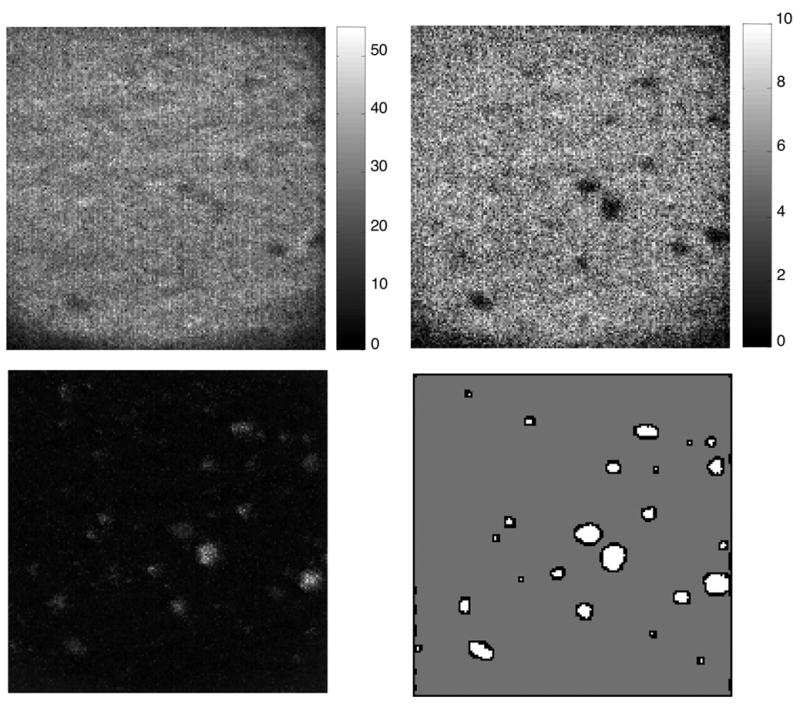
250 micron × 250 micron image of atmospheric aerosol particles on a Teflon filter. The total ion image is shown at the upper left and CF⁺ image is shown on the upper right. The image for MAF factor 1 is shown on the lower left and at the lower right the region definitions used to calculate image contrast are shown.

Figure 2.

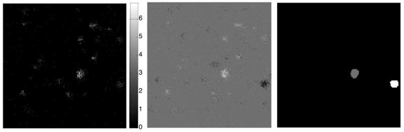
250 micron × 250 micron image of atmospheric aerosol particles on a Teflon filter. Ca⁺ image (left), MAF factor 3 image (center), and region definitions for the two particles (right) are shown.

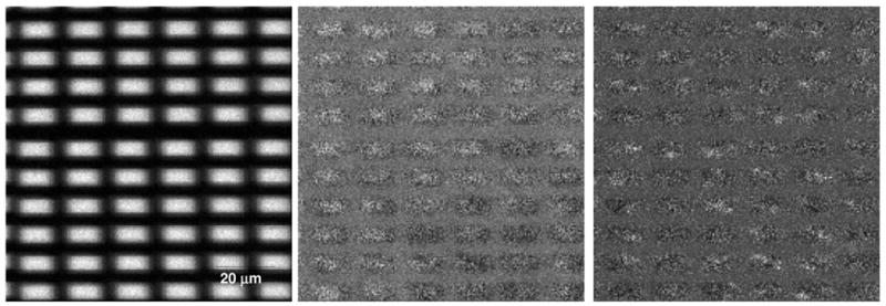
Image 2 (figure 3) consists of proteins adsorbed onto alkanethiol covered gold islands. Prior to protein adsorption the silicon regions surrounding the gold islands were back-filled with PLL-g-PEG. This image is complicated by a strong matrix effect from the gold regions which leads to an enhancement of all ion intensities and overall low ion counts. Because the matrix effect is highly spatially correlated with the protein islands, it is very difficult to ascertain whether there is a real chemical difference between the surface organic species on the islands and the surface organic species between the islands. Figure 3 shows the total ion image with region definitions (left), the best contrast obtainable by a single normalized peak (center) and the MAF factor 2 image for the normalized data (right). As can be seen in Table 2, when mean centering is used without normalization, contrast between the PEO regions and protein regions is observed but the factor loadings that result in this contrast show no significant correlation with the spectral features of interest. If either normalization is used or no mean centering is done, the chemical contrast between the two regions is separable from the matrix effect.

Figure 3.

ToF-SIMS images of the protein/PEG patterned surface. On the left, the total ion image is shown with the protein and PEO regions outlined. In the center is the normalized mass 63 image, which shows the highest contrast of any single peak following normalization. On the right is shown MAF factor 1 image calculated from the normalized data.

Table 2.

PCA and MAF Results for Mean Centered Data

Sample	criteria	no scaling	auto scalin	filter-scaling	root mean	shift variance	MAF
Aerosol Particles
Filter/Particles	Factor #	1	1	1	1	1	1
	contrast	2.109	5.302	2.671	5.791	5.645	5.904
Particles	Factor #	35	3	39	3	3	3
	contrast	2.114	2.139	0.9792	2.061	2.103	2.155
Protein/PEG pattern	Factor #	2	2	1	2	2	1
	contrast	0.5391	1.387	1.4858	1.444	1.4435	1.7131
	Spectra	0.4349	0.4587	0.4735	0.4545	0.451	0.4631
Protein/PEG pattern
Bars	Factor #	1	1	1	1	1	1
	contrast	9.143	9.542	9.549	9.768	9.749	9.754
Organics	Factor #	2	3	2	5	2	2
	contrast	0.6152	0.0639	0.9404	0.2773	0.7763	2.042
Salts	Factor #	7	8	10	3	8	3
	contrast	0.178	0.1723	0.0353	0.6105	0.5225	2.371

Image 3 (figures 4 and 5) consists of polystyrene microspheres. Adsorbed BSA is present on some of the spheres, while adsorbed HSA is present on others. This image presents significant challenges. The first is topography. As can be seen in the total ion image (figure 4 upper left), there are dramatic differences in the total ion yield across the surfaces of each sphere. These topographic effects mask the chemical differences between the samples (see region definitions in figure 4, lower right) as is illustrated by the 72 m/z peak image (figure 4, upper right). Mass 72 shows the strongest contrast between the two different types of spheres for an individual peak. The MAF 2 image from the mean centered data (figure 4, lower left) shows clear contrast between the two proteins and the factor loadings are highly correlated with the key protein peaks. Unfortunately, in figure 4 the contrast can only be observed along the bright edge of the spheres because of the topographic effects. These effects can be reduced by normalizing the images to total ion yield. Figure 5 shows the MAF factor 2 image calculated using normalized mean centered data. After normalizing to the total ion image, the contrast between two proteins can be visualized over most of the sphere surface.

Figure 4.

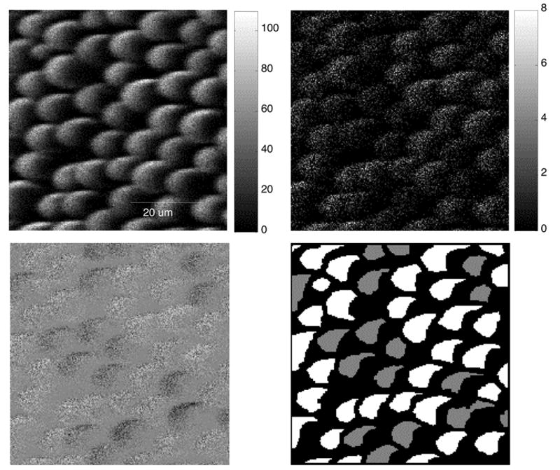
ToF-SIMS images of 10 micron protein coated polystyrene spheres. Total image (upper left), mass 72 image (upper right), MAF factor 2 image (lower left), region definitions for the two proteins (lower right) are shown.

Figure 5.

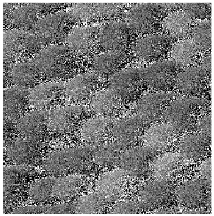
MAF factor 2 from the normalized ToF-SIMS image of 10 micron protein coated polystyrene spheres.

Image 4 has a much higher overall intensity than the other images explored, with 2.8e7 total counts and an average of 463 total counts per pixel. In this image, with 964 peaks, nearly 20% of the counts come from the Cs⁺ ion which alone shows a dramatic contrast of 8.64 between the protein/alkyl thiol/gold islands and the PLL-g-PEG/silicon background regions. Once again, the matrix effect of the gold is so strong that all of the spectral peaks, except Al and K, are dramatically enhanced on the islands. As a result, clear contrast between the islands and background can be obtained with virtually every peak in the spectrum. The challenge in this image is not in visualizing the islands, but in determining if there are any other structures in the image. Figure 6 shows the first three MAF images obtained from this data set. MAF factor 1 (left) shows the dramatic contrast between the gold islands and the silicon. MAF factor 2 (center) shows bright organic rich regions and darker regions where the gold and Cs are more visible through the overlayer. This image can be very faintly detected in PCA with root mean scaling or shift variance scaling but not with any of the other scaling methods. MAF factor 3 (right) shows spots of sodium and potassium on the image. Curiously, although these spots can be clearly visualized in the single ion images for Na⁺ and K⁺, they can not be visualized in any of the PCA processed images. For this image, when the data was normalized no features other than the clearly distinguished gold islands could be identified in any of the MAF or PCA images.

Figure 6.

MAF images from the protein/PEG patterned surface. On the left is MAF factor 1, which shows variations in total ion yield across the sample. In the center is MAF factor 2, which shows non-uniform coating of organic species (bright) on the gold rectangles. On the right is MAF factor 2, which shows the salt contaminants on the surface (bright spots).

5 Discussion

By comparing the data in the four tables, it can be seen that normalization was an effective aid for deconvoluting matrix or topographic effects from chemical differences. In the absence of strong matrix or topographical effects (particles sample), normalization provided little benefit with added computational complexity. It should be noted that when normalization is used without mean centering, the first factor is always a noise image that shows no significant image contrast and therefore normalized data should always be mean centered to achieve optimal results.

When the data is not mean centered, the first factor always describes differences in the data means. In most cases, mean centering simply reduced the number of factors needed to describe the data with little change in the resulting image contrast. The key exception to this was for the protein/PEG sample where the matrix effects that influenced total ion yield were strongly correlated with the chemistry of the organic overlayer. In this case, peaks revealing the differences in the overlayer chemistry could be identified in the un-preprocessed data set, but were lost when mean scaling was employed. This occurred because the factors are required to be orthogonal to each other. When the data is mean centered but not normalized, the first factor typically describes variations in the total ion yield. In this case those variations were nearly parallel to the variations due to overlayer chemistry so no vector that is orthogonal to the total ion yield is able to capture the overlayer chemistry. When the data is not normalized, the first factor will describe the image mean. In this case, the image mean appears to be less strongly correlated with the differences in overlayer chemistry than the total ion yield. As a result, the potential remained for finding a factor that described only the overlayer chemistry.

Both normalization and mean centering increase the memory requirements for the calculations. The raw image files are sparse and contain only integer values, so the data can be efficiently stored in computer memory by use of sparse matrix routines and/or integer formats. When the data is normalized, it must be stored as floating point values. When it is mean centered, it is no longer sparse. For the images explored here, these were not limiting factors in the analysis, but they will become issues in the processing of larger images at higher mass resolution and in three dimensional imaging.

As can be seen in Tables 1 – 4, MAF produced the best results in terms of reducing the size of the data set, improving image contrast and recovering spectral features for all cases. To recover spectral features with MAF, however, it is necessary to use the inverted loadings. A direct comparison of the loadings to the spectra shows a very poor correlation ¹¹. It should be noted, however, that PCA with root mean scaling and shift variance scaling often perform very nearly as well as MAF, while the un-scaled data with PCA was typically far worse than any of the scaling methods investigated.

Because PCA seeks to maximize variance between the pixels, ion peaks which vary over a larger range will dominate the analysis. This will only result in physically and statistically meaningful results if the variance in each peak is directly comparable. There is a growing consensus, within the statistical community, that PCA is most logically applied when variables are scaled based on their measurement uncertainty ¹³. If the data can be accurately scaled by their measurement uncertainty, those variables that vary over many times their measurement uncertainty will dominate the PCA analysis while those whose variance is within the noise will be minimized, a result which is pleasing from both a chemical and statistical standpoint.

For spectroscopic techniques that rely on counting particles, such as ToF-SIMS, the observed noise increases in absolute intensity as the number of counts increase. The result is that the absolute measurement uncertainty for intense peaks is greater than the measurement uncertainty for weak peaks. If PCA is performed on the raw counts, intense peaks which vary only due to noise generally dominate over important weaker peaks. This effect is consistent with the poor results obtained for all of these images when the un-scaled data was processed.

Unfortunately, the measurement uncertainty is often not known and it may differ from pixel to pixel as well as from peak to peak. In this paper we have compared auto-scaling, root mean scaling, filter scaling, and shift variance scaling for four images using four different preprocessing approaches. For many cases, the differences between auto-scaling, root mean scaling and variance scaling are small and all provide significant improvement of the un-scaled data.

Auto-scaling consists of dividing each peak by the standard deviation of that peak over the image. If there are no features in the image, the standard deviation will be an accurate estimate of the measurement uncertainty. But, of course, images with no features are not of primary concern. In the presence of image features the standard deviation will include both variance due to the features and variance due to noise and will therefore be typically greater than the measurement uncertainty. As a result, auto-scaling has a tendency to amplify noise peaks relative to peaks which show image contrast. The one exception to this rule is in the case of very sparse features such as the particles on the Teflon filter where auto-scaling yields the maximum contrast between the two particles. If a peak has zero counts in all but a small region of the image, the standard deviation will underestimate the measurement error for this region and therefore amplify this region in the analysis. It should be noted, however, that auto-scaling does not include any information about neighborhood, so 20 intense pixels scattered randomly across the sample will be amplified to exactly the same extent as 20 intense pixels in one tight region.

Root mean scaling consists of dividing each peak by the square root of the mean value for that peak. Root mean scaling is derived from the assumption that the image noise is Poisson in nature so the measurement uncertainty is equal to the square root of the counts ¹³. If the data is truly Poisson distributed and there are no features in the image, the square root of the mean will be an accurate estimate of the measurement uncertainty. For peaks that vary only due to Poisson noise, root mean scaling will be identical to auto-scaling. When there are features in the image, the image mean will fall between the means for the different regions and the square root of the mean will typically be smaller than the standard deviation about the mean. As a result, root mean scaling appears to provide a better estimate of the measurement uncertainty than auto-scaling for most cases and therefore will yield better PCA results. The exception to this is when the Poisson assumption is badly violated. This occurs when data is normalized and is most obvious on the protein coated spheres where root mean scaling yields the worst results of all the methods.

Filter scaling consists of dividing each peak by a standard deviation for that peak which is calculated by excluding pixels which have zero counts and no non-zero neighbors ²⁴. Filter scaling will be identical to auto-scaling if there are few zeros in the image and will show the most dramatic difference from the other scaling methods for very low count rate images. Because pixels which are zero and surrounded by zeros are excluded in the calculation of the scaling factors, the standard deviation for sparsely distributed peaks will be over-estimated and so the influence of these peaks will be diminished in the image. This will have the effect of reducing salt and pepper noise in the PCA images. In the protein/PEG image, which has a large number of zeros, this proves an advantage and filter scaling performs the best at reducing the number of factors require to visualize the image contrast.

In contrast, if a peak is present in one region of interest, but absent in other regions of the image, filter scaling will provide an accurate estimate of the measurement uncertainty in the region of interest, but will over-estimate the pooled uncertainty for all regions. As a result, filter scaling should be worse for detecting features that constitute only a tiny fraction of the image, an outcome which is observed for the particles on the Teflon filter.

Shift variance scaling is inspired by MAF and so it is not surprising that it often achieves very similar results to MAF. It is based on the assumption that most image features are much larger than a single pixel and therefore neighboring pixels will differ primarily due to their measurement uncertainty. The standard deviation in the shift matrix should provide an accurate estimate of the true pooled measurement uncertainty if the pixels bordering regions of image contrast constitute only a small fraction of the image, a condition which is nearly always met. If there is no covariance between peaks in the shift image, shift variance scaling and MAF should yield identical results. The fact that MAF consistently provides improved performance over shift variance scaling suggests that the covariance of peaks in the shift image, although generally small, plays an important role. The advantages of MAF are most evident in detecting subtle features, such as the contrast between HSA and BSA, two very similar proteins, or the small non-uniformities in the organic layers on the gold islands. This advantage is of particular significance since these subtle features are often the most difficult to detect using a univariate image processing approach.

6 Conclusions

PCA, with four different scaling options, and MAF have been tested on four ToF-SIMS images. Additionally, normalization and mean centering were explored as pre-processing options. A summary of the image contrast and spectral recovery results, averaged over all four images, is shown in Table 5. The image contrast values for a given image and set of pre-processing conditions were ratioed to the best value for that particular image and pre-processing conditions. Then the average value was calculated for each set of processing conditions using from the results from all four images. The spectral recovery values in Table 5 are just the average of the correlation coefficients from the four images at each set of pre-processing conditions. For all of the images and all of the pre-processing options, MAF produced the best results in terms of reducing the dimensionality of the data, enhancing image contrast and recovering key spectral features. MAF showed particular strength for identifying subtle features that were often lost in PCA and impossible to visualize in single peak images.

Table 5.

Average PCA and MAF Image Contrast and Spectral Recovery for the Four ToF-SIMS Images

	no preprocessing	mean centering	normalization	mean centering and normalization
Image Contrast (average fraction of best case)
no scaling	0.5229	0.4844	0.5608	0.4919
Auto	0.6800	0.6602	0.9129	0.8953
filter-scaling	0.5575	0.5851	0.6323	0.5663
root mean	0.7832	0.7333	0.8557	0.7085
shift variance	0.7475	0.7646	0.9119	0.8842
MAF	1.0000	1.0000	1.0000	1.0000
Average Spectral Recovery
no scaling	0.3889	0.4008	0.4008	0.6517
Auto	0.9330	0.8803	0.8803	0.8581
filter-scaling	0.9274	0.6068	0.6068	0.7403
root mean	0.9713	0.6159	0.6159	0.6763
shift variance	0.9729	0.9045	0.9045	0.8842
MAF	0.9889	0.9330	0.9330	0.9491

Normalization proved an important tool for deconvoluting chemical effects from topographic and/or matrix effects. Mean centering aided in reducing the dimensionality of the data, but in one case resulted in a loss of information.

Although MAF outperforms all of the scaling methods with PCA, it should be noted that MAF is more computationally intensive and requires more computer memory. For the images investigated, MAF took 2 to 5 times more computer time than PCA with scaling. Although this was not a limiting factor for this study, the shorter computing times may become important for the analysis of high mass resolution images and three dimensional images. Root mean scaling and shift variance scaling can provide very similar results to MAF and may therefore be strong alternatives to MAF for the analysis of very large images. Filter scaling may have a nitch for analysis of very low count rate images.

Table 3.

PCA and MAF Results for Normalized Data

Sample	criteria	no scaling	auto scaling	filter-scaling	root mean	shift variance	MAF
Aerosol Particles
Filter/Particles	Factor #	1	2	1	2	2	2
	contrast	2.3419	6.4	3.7567	6.4243	6.4927	6.4817
Particles	Factor #	33	4	39	3	4	4
	contrast	1.7727	2.4581	0.9727	2.0595	2.0577	2.2045
Protein/PEG pattern
	Factor #	1	5	2	5	5	2
	contrast	0.5784	0.9762	0.9526	1.0001	1.0016	1.1567
	Spectra	0.528	0.9587	0.9476	0.9644	0.9707	0.9981
Protein Spheres	Factor #	1	2	1	1	2	2
	contrast	0.4743	0.5789	0.5621	0.5196	0.6949	0.8209
	Spectra	0.2735	0.8019	0.266	0.2674	0.8383	0.8678

References

- 1.Sosnik A, Sodhi RN, Brodersen PM, Sefton MV. Surface study of collagen/poloxamine hydrogels by a ‘deep freezing’ ToF-SIMS approach. Biomaterials. 2006;27:2340–2348. doi: 10.1016/j.biomaterials.2005.11.028. [DOI] [PubMed] [Google Scholar]
- 2.Zhang Z, Ma H, Hausner DB, Chilkoti A, Beebe TP., Jr Pretreatment of Amphiphilic Comb Polymer Surfaces Dramatically Affects Protein Adsorption. Biomacromolecules. 2005;6:3388–3396. doi: 10.1021/bm050446d. [DOI] [PubMed] [Google Scholar]
- 3.Zhang Z, Yoo R, Wells M, Beebe TP, Jr, Biran R, Tresco P. Neurite outgrowth on well-characterized surfaces: preparation and characterization of chemically and spatially controlled fibronectin and RGD substrates with good bioactivity. Biomaterials. 2005;26:47–61. doi: 10.1016/j.biomaterials.2004.02.004. [DOI] [PubMed] [Google Scholar]
- 4.Belu AM, Graham DJ, Castner DG. Time-of-flight secondary ion mass spectrometry: techniques and applications for the characterization of biomaterial surfaces. Biomaterials. 2003;24:3635–53. doi: 10.1016/s0142-9612(03)00159-5. [DOI] [PubMed] [Google Scholar]
- 5.Goessl A, Garrison MD, Lhoest JB, Hoffman AS. Plasma lithography — thin-film patterning of polymeric biomaterials by RF plasma polymerization I: Surface preparation and analysis. Journal Biomater Sci Polym Ed. 2001;12:721–38. doi: 10.1163/156856201750411620. [DOI] [PubMed] [Google Scholar]
- 6.Graham DJ, Wagner MS, Castner DG. Information from Complexity: Challenges of ToF-SIMS Data Interpretation. Applied Surface Science. 2006;252:6860–6868. [Google Scholar]
- 7.Gillen G, Fahey A. Secondary ion mass spectrometry using cluster primary ion beams. Applied Surface Science. 2003;203–204:209–213. [Google Scholar]
- 8.Weibel D, Wong S, Lockyer N, Blenkinsopp P, Hill R, Vickerman JC. A C60 Primary Ion Beam System for Time of Flight Secondary Ion Mass Spectrometry: Its Development and Secondary Ion Yield Characteristics. Analytical Chemistry. 2003;75:1754–1764. doi: 10.1021/ac026338o. [DOI] [PubMed] [Google Scholar]
- 9.Postawa Z, Czerwinski B, Szewczyk M, Smiley EJ, Winograd N, Garrison BJ. Microscopic Insights into the Sputtering of Ag{111} Induced by C60 and Ga Bombardment. Journal of Physical Chemistry B. 2004;108:7831–7838. doi: 10.1021/jp050821w. [DOI] [PubMed] [Google Scholar]
- 10.Wagner MS, Graham DJ, Castner DG. Simplifying the Interpretation of ToF-SIMS Spectra and Images using Careful Application of Multivariate Analysis. Applied Surface Science. 2006;252:6575–6581. [Google Scholar]
- 11.Tyler BJ. Multivariate Statistical Image Processing for Molecular Specific Imaging in Organic and Biological Systems. Applied Surface Science. 2006;252:6875–6882. [Google Scholar]
- 12.Willse A, Tyler B. Poisson and Multinomial Mixture Models for Multivariate SIMS Image Segmentation. Anal Chem. 2002;74:6314–22. doi: 10.1021/ac025561i. [DOI] [PubMed] [Google Scholar]
- 13.Keenan MR, Kotula PG. Accounting for Poisson noise in the multivariate analysis of ToF-SIMS spectrum images. Surface and Interface Analysis. 2004;36:203–212. [Google Scholar]
- 14.Nygren H, Malmberg P. Silver deposition on freeze-dried cells allows subcellular localization of cholesterol with imaging TOF-SIMS. Journal of Microscopy. 2004;215:156–161. doi: 10.1111/j.0022-2720.2004.01374.x. [DOI] [PubMed] [Google Scholar]
- 15.Biesinger MC, Paepegaey P-Y, McIntyre NS, Harbottle RR, Petersen NO. Principal Component Analysis of TOF-SIMS Images of Organic Monolayers. Anal Chem. 2002;74:5711–5716. doi: 10.1021/ac020311n. [DOI] [PubMed] [Google Scholar]
- 16.Smentkowski VS, Keenan MR, Ohlhausen JA, Kotula PG. Multivariate Statistical Analysis of Concatenated Time-of-Flight Secondary Ion Mass Spectrometry Spectral Images. Complete Description of the Sample with One Analysis. Anal Chem. 2005;77:1530–1536. doi: 10.1021/ac048468y. [DOI] [PubMed] [Google Scholar]
- 17.Wolkenstein M, Hutter H, Mittermayr C, Schiesser W, Grasserbauer M. Classification of SIMS Images Using a Kohonen Network. Anal Chem. 1997;69:777–782. [Google Scholar]
- 18.Wagner MS, Graham DJ, Ratner BD, Castner DG. Maximizing Information Obtained from Secondary Ion Mass Spectra of Organic Thin Films Using Multivariate Analysis. Surface Science. 2004;570:78–97. [Google Scholar]
- 19.Wold S, Esbensen K, Geladi P. Principal Component Analysis. Chemometrics and Intelligent Laboratory Systems. 1987;2:37–52. [Google Scholar]
- 20.Green AA, Berman M, Switzer P, Craig MD. A transformation for ordering multispectral data in terms of image quality with implications for noise removal. IEEE Transactions on Geoscience and Remote Sensing. 1988;26:65–74. [Google Scholar]
- 21.Larsen R. Decomposition using maximum autocorrelation factors. Journal of Chemometrics. 2002;16:427–435. [Google Scholar]
- 22.McLachIan GJ. Discriminant Analysis and Statistical Pattern Recognition. Wiley; New York: 1992. Chapter 13. [Google Scholar]
- 23.McCuliagh P, Nelder JA. Generalized Linear Models. 2. Chapman & Hall; London: 1989. Chapter 6. [Google Scholar]
- 24.Rayal G. MS Thesis. Department of Chemical Engineering; University of Washington: 2006. Multivariate Analysis and Enhancement of ToF-SIMS Images from Biomolecular Patterns at Micron- and Nanometer Scale. [Google Scholar]
- 25.Veiseh M, Zhang Y, Hinkley K, Zhang M. Two-Dimensional Protein Micropatterning for Sensor Applications Through Chemical Selectivity Technique. Biomedical Microdevices. 2001;3:45–51. [Google Scholar]
- 26.Veiseh M, Wickes BT, Castner DG, Zhang MQ. Guided cell patterning on gold–silicon dioxide substrates by surface molecular engineering. Biomaterials. 2004;25:3315–3324. doi: 10.1016/j.biomaterials.2003.10.014. [DOI] [PubMed] [Google Scholar]
- 27.Michel R, Lussi JW, Csucs G, Reviakine I, Danuser G, Ketterer B, Hubbell JA, Textor M, Spencer ND. Selective Molecular Assembly Patterning: A New Approach to Micro-and Nanochemical Patterning of Surfaces for Biological Applications. Langmuir. 2002;18:3281–3287. [Google Scholar]
- 28.Kenausis GL, Voros J, Elbert DL, Huang NP, Hofer R, Ruiz-Taylor L, Textor M, Hubbell JA, Spencer ND. Poly(L-lysine)-g-Poly(ethylene glycol) Layers on Metal Oxide Surfaces: Attachment Mechanism and Effects of Polymer Architecture on Resistance to Protein Adsorption. Journal of Physical Chemistry B. 2000;104:3298–3309. [Google Scholar]
- 29.Huang NP, Michel R, Voros J, Textor M, Hofer R, Rossi A, Elbert DL, Hubbell JA, Spencer ND. Poly(L-lysine)-g-poly(ethylene glycol) Layers on Metal Oxide Surfaces: Surface-Analytical Characterization and Resistance to Serum and Fibrinogen Adsorption. Langmuir. 2001;17:489–498. [Google Scholar]
- 30.Rangarajan S, Tyler BJ. Interpretation of Static Time-of-flight Ion Mass Spectral Images of Adsorbed Protein Films on Topographically Complex Surfaces. Applied Surface Science. 2004;231–232:406–410. [Google Scholar]
- 31.Tyler BJ, Brüning C, Rangaranjan S, Arlinhaus HF. manuscript in preparation. 2006. [Google Scholar]