Image Correlation Algorithm for Measuring Lymphocyte Velocity and Diameter Changes in Contracting Microlymphatics

Abstract

Efforts have recently been made to estimate wall shear stress throughout the contractile cycle of mesenteric rat lymphatics with a high speed video microscopy system. This was prompted by reports in the literature that lymphatic pumping is related to wall shear stress. While one can estimate wall shear stress by tracking lymphocyte velocity, it is prohibitively tedious to manually track particles over a reasonable time frame for a good number of experiments. To overcome this, an image correlation method similar to digital particle imaging velocimetry was developed and tested on contracting lymphatics to measure both vessel diameter and fluid velocity. The program tracked temporal fluctuations in spatially averaged velocity with a standard error of prediction of 0.4 mm/s. From these studies we have measured velocities ranging from −2 to 4 mm/s. Diameter changes were also measured with a standard error of 7 μm. These algorithms and techniques could be beneficial for investigating various changes in contractile behavior as a function of changes in velocity and wall shear stress.

INTRODUCTION

The lymphatic system plays a crucial role in the transport of proteins and large particulate matter away from the interstitial spaces in the body, since the capillaries cannot move such particles directly by absorption. In addition to tissue homeostasis, the lymphatic system also plays important, although not completely understood, roles in lipid transport and metabolism, and immune function.⁶ Recent findings have shown that the primary mechanism for promoting flow through the mesenteric lymphatics, the spontaneous phasic contractions of the lymphatic wall known as the intrinsic lymphatic pump, exhibit a wall shear stress dependency. Specifically, both the frequency and amplitude of vessel contraction is inhibited by high fluid flow through the vessel.^4,5 This observation prompted a need to measure the velocity dynamics in these vessels throughout the contraction cycle, so as to develop an estimation of the shear stresses that occur in situ. The recent development of a high speed imaging system to measure lymphatic flow and estimate wall shear stress has now opened up a new area of research in lymphatic microcirculation.^2,3 The main difficulty with this system has been the tedious post-processing required to analyze the large amount of data produced by the high speed imaging (500 frames per second (fps)). To put this into perspective, the findings recently published by Dixon,² which corresponded to data taken from seven rats for a total of about 24 min or approximately 288,000 images, took over a year and a half to analyze. Not only is this expensive in terms of man hours, it is also difficult to perform various other flow-related studies when the results take so long to process. Pre-packaged particle tracking software produced spurious results due to the inherent low contrast of the imaging site. Contrast could be improved through the injection of fluorescent tracers; however, that would be undesirable given the influences such injections could have on tissue homeostasis and the lack of a low-light/hi-speed video camera. These limitations led us to seek out an image analysis technique to calculate the fluid velocities automatically without having to introduce fluorescent tracers into the system.

Recently, Tsukada⁸ reported an image correlation method combined with a high speed imaging system that could measure the flow of erythrocytes in small capillaries (<50 μm in diameter). This method relies on measuring the displacement of a particular red cell distribution pattern between image frames through the use of the correlation function. We have adapted this method for our high speed imaging system to simultaneously measure lymphatic flow and vessel diameter. With this innovation, an image sequence that would normally take over a week to analyze manually can be processed automatically with a high degree of accuracy in less than 30 min.

MATERIALS AND METHODS

Animal Protocol

Eight male Sprague–Dawley rats weighing 180–220 g were imaged using the high speed imaging system described previously at a frame rate of 500 fps.³ The rats were housed in an environmentally controlled, American Association for Accreditation of Laboratory Animal Care-approved vivarium. All animal protocols followed were approved by ULACC/IAACUC. Each animal was fasted for 12–15 h before the experiments, while water was available ad libitum. Each rat was anesthetized with an intramuscular injection of Fentanyl-Droperidol (0.3 ml/kg) and Diazepam (2.5 mg/kg). Supplemental doses of the anesthetic were given as needed. An abdominal incision was made to gain access to the mesenteric lymphatic vessels. A loop of the small intestine was exteriorized through the incision and gently positioned over a semicircular viewing pedestal on a Plexiglas preparation board capable of maintaining temperature and superfusing the vessel with a heated buffered solution. A lymphatic vessel was centered over an optical window in the preparation board. The exteriorized tissue was superfused with a phosphate buffered solution supplemented with HEPES (10 mM) and 1% bovine serum albumin. The solution was pre-warmed to 38°C, and the pH adjusted to 7.4. The temperature of the exteriorized tissue and the animal’s core were maintained at 36–38°C. The preparation board was placed on the stage of an intravital microscope (Zeiss), and the lymphatic vessel was observed at a magnification of 100–200 × using an 80 mm projective lens, a 10 × water immersion objective, and a variable magnification intermediate lens. The depth of field for this optic setup was approximately 14 μm. All the experiments were digitized with the high-speed video camera (Dalstar64K1M, 1M fps 245 × 245, CCD camera). The experimental images from these rats were recently used and published,² however only those image sets that had a large lymphocyte density were used in this report with this algorithm due to the algorithm’s dependency on a certain number of particles in the correlation window.

Measuring Lymph Flow Velocity

The velocity estimation technique involves the cross-correlation of sequential image pairs from the high-speed camera, and is similar to that presented by Tsukada.⁸ One of the main difficulties of automated image analysis of lymphocyte movement in these lymphatic vessels is the poor contrast inherent to these images (Fig. 1). In order to overcome this obstacle, we took two sequential images separated by 2 ms and subtracted them from one another. This subtraction enhanced pixels in motion, while canceling out the motionless background. Given our sampling rate and magnification, the resulting image would only show particles moving faster than about 0.25 mm/s, and would filter out the “motionless” background (motion less than 0.25 mm/s). In our previous work,² we measured the motion artifact from vessel drift and the velocity of wall contractions to usually be well under 0.25 mm/s.

FIGURE 1.

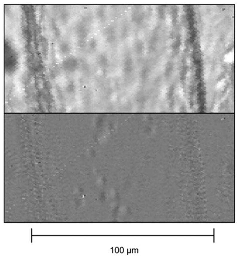
Portion of a lymphatic vessel before (top) and after (bottom) image subtraction and low pass filtering. One can see that the lymphocytes are much easier to distinguish in the bottom image.

The subtraction described above was repeated with another pair of images taken 8 ms after the first pair, and the two resultant images were then processed through a low pass filter to remove high frequency noise due to pixel to pixel variations. Each of these filtered images was then used in the image correlation algorithm. A total of four raw images were used to calculate the fluid velocity as shown by the following Eqs. 1–3:

$$\text{Picf}=\text{LPF}(\text{Pic}1-\text{Pic}2)$$ (1)

$$\text{Picg}=\text{LPF}(\text{Pic}3-\text{Pic}4)$$ (2)

$$\begin{array}{l}\text{CCOR}(k,l)=\left(\frac{1}{N}\sum _{m=0}^{N-1}(f_m(x,y)-\overline{f})(g_m(x+k,y+l)-\overline{g})\right)\\ \times (\frac{1}{N}\sum _{m=0}^{N-1}{(f_m(x,y)-\overline{f})}^2\frac{1}{N}\\ {\sum _{m=0}^{N-1}{(g_m(x+k,y+l)-\overline{g})}^2)}^{-1/2}\end{array}$$ (3)

In the above equations, Pic2 and Pic3 are separated by 4 ms, f_m (x, y) corresponds to a given pixel within the window created in Picf, g_m (x, y) corresponds to a given pixel in Picg, f̄ is the mean of window f_m, and ḡ is the mean of window g_m. LPF refers to the low pass filter used on the subtracted images. CCOR is the two dimensional cross correlation function where CCOR(k, l) refers to a single correlation coefficient after one window has been displaced k and l pixels in the horizontal and vertical direction, respectively. The window in image Picf was fixed, while the window in Picg was scanned across the picture to find the location of maximum correlation. This resultant window displacement, when combined with the known frame rate, gives a measure of the fluid velocity (Fig. 2). The main limitation found in using this approach with lymphatic vessels, is that the particle densities are much lower than those found in the blood, or in a fluid seeded with particles for this purpose. Due to this limitation, we found that the best results were produced with a window size approaching at least half of the vessel diameter. In hindsight, we found that the correlation algorithm needed at least three lymphocytes within the window to consistently measure velocity with a sufficient correlation coefficient. Given our field of view and average vessel diameter this corresponds to a lymphocyte density of approximately 2,000 cells/μl. Lymphocyte density is usually high enough to meet this minimum criterion although this is not always the case.² All analysis was done in Matlab after capturing images with a high speed camera (frame rate of 500 fps). This frame rate was established as optimal in our previous studies.³

FIGURE 2.

Illustration of the principle of the image correlation approach. Each image is taken at the same location separated by a small time interval. The displacement of the window corresponds to the movement of the fluid.

Measuring Vessel Diameter

The program was then modified to measure changes in vessel diameter. The program first provides an image for the user to select the left and right vessel wall on the image. The program then creates two reference windows around each of the selected locations. The displacements of these windows are measured by finding the maximum correlation in a sequential image as governed by Eq. 3. From the coordinates of these two windows, the vessel diameter can be measured through a simple subtraction (Fig. 3). The displacement of the two windows averaged together gives information about motion artifact and overall image drift, which proves useful for improving the algorithm as described in the next section.

FIGURE 3.

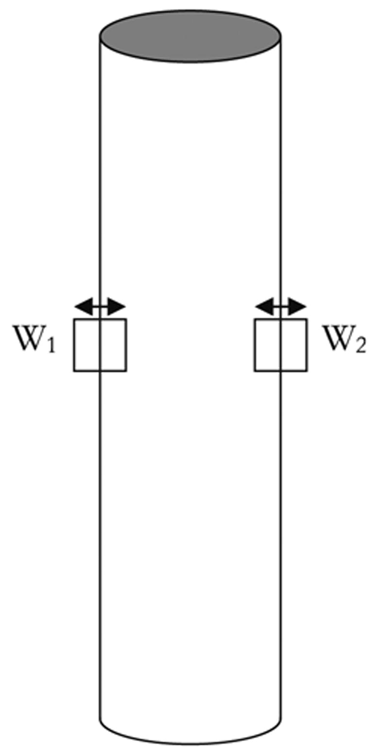
Two reference windows are created around each of the vessel walls in the same vertical location. Their displacements are tracked to measure changes in vessel diameter.

Optimizing the Image Correlation Algorithm

After initial analysis, several improvements were made to the code. It was noted that the maximum correlation location occasionally produced erroneous outliers in the velocity tracings. To improve the tracking, a measure of the relative correlation was introduced into the algorithm by taking the ratio of the peak correlation value with the average of its surrounding values (Fig. 4). As can be seen by visually comparing Fig. 4a with Fig. 4b, the location of maximum correlation in Fig. 4a is an acceptable match, while the location of maximum correlation in Fig. 4b is just noise, because the ratio of the peak with that of the area surrounding the peak is very small. We rejected all matches that produced a ratio less than five, which was a very conservative number, chosen to ensure that no incorrect matches were made while only occasionally discarding what was an acceptable match. Whenever an erroneous match was discovered, as in the example above, that value was replaced with an average of the velocities occurring before and after the event.

FIGURE 4.

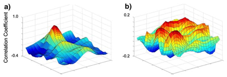
Correlation coefficient values for various window locations from Picg. Note the extent of the maximum as compared with the rest of the surface: (a) would be considered an acceptable match due to the ratio of the peak to its surroundings; (b) would be considered a poor match.

Another problem encountered was that of motion artifact due to sudden movements by the animal or the occasional transmission of intestinal motility to the imaging site. Since the magnification was so large, even the smallest movements could cause problems. Initially the velocity reference window created was not dynamic, but was fixed in the same location for each given sequence during analysis. This made window matching difficult or even irrelevant if the window drifted partially or sometimes completely outside of the vessel. To correct this, the velocity calculations were implemented after the diameter measurements were made, so that the reference window could always be placed in the center of the diameter. This also allowed us to change the width of the window to match the vessel’s diameter (0.8*diameter), since as noted before, a larger window size improves the chances of an acceptable match.

We also sought to improve the speed of analysis from a computational standpoint. Originally we had to scan the entire image because the vessel itself would shift around in the field of you. However, after the above changes were made we were able to reduce the scan size because motion artifact was compensated for. By referencing the vessel orientation and direction of flow in the sequence being analyzed and combining it with the known parameters of the velocity ranges that occur in vivo with the frame rate and magnification, we calculated the maximum pixel displacement that the correlation window could undergo from one frame to the next. We could then limit the size of the correlation scan to a value 20% greater than the maximum displacements (± 4 pixels in the direction orthogonal to flow and + 80/−24 pixels in the direction parallel to flow).

RESULTS AND DISCUSSION

In Situ Experiments

Estimations of lymphocyte velocity were in most cases very reliable, with the occasional presence of noise. The program successfully picked out dynamic fluctuations in velocity; however, there are numerous segments of data that appear to be noise (Fig. 5a). The standard error of prediction for this case sequence was 0.85 mm/s. While one could easily remove the points classified as “noise” after comparing them with the manually tracked data, the improvements described in the previous section were implemented to improve the noise level consistently without having to use the manual data analysis.

FIGURE 5.

(a) Comparison of spatially averaged velocity calculated from manually tracked data with that of the correlation algorithm before adaptive filtering, Standard Error of Prediction (SEP) = 0.85 mm/s; (b) Comparison of spatially averaged velocity calculated from manually tracked data with that calculated by the correlation algorithm after modifications were made to improve the algorithm, SEP = 0.50 mm/s; (c) Comparison of maximum velocity calculated from manually tracked data with that calculated by the correlation algorithm after modifications were made to improve the algorithm, SEP = 0.49 mm/s; (d) Comparison of the optimized velocity (V* =W × V_max + (1 − W) V̄) calculated from manually tracked data with that calculated by the correlation algorithm, SEP = 0.43 mm/s.

As described in the materials and methods section, one other modification that was made to improve the lymphocyte velocity measurements was to create a method for removing “bad” data points by comparing the correlation coefficient at the best fit with the correlation coefficients spatially surrounding that fit. This, in conjunction with the dynamic reference window, improved the data dramatically (Fig. 5b).

One question that arises from this is whether or not the displacement of the reference window found by the program is actually a measure of spatially averaged velocity (V̄) (assuming that the spatially averaged velocity V̄ is half of the maximum velocity (V_max), as would be the case for cylindrical tube Poiseuille flow). This should be the case if there is an even distribution of lymphocytes across the radius of the vessel. However, if there are more lymphocytes in the center of the vessel than near the wall, the displacement of the window would approach the center velocity (i.e., V_max) instead (Fig. 5c).

Of course, in order for V_max to be the best match, all of the tracked lymphocytes would have to be in the center, which is unlikely to be the case if there is more than one lymphocyte located in a given cross section of the vessel. It seems logical then, that the physical representation of the velocity calculated by the correlation algorithm is larger than V̄ (since particles tend to locate themselves near the center) and lower than V_max (since all of the particles cannot flow through the center). To see if this is the case for this particular data set, a program was written in Matlab to vary the velocities calculated from the manually tracked data from V̄ to V_max, while keeping the correlation tracked velocities the same, and find the minimum standard error of prediction for the correlation method (Fig. 6). For this particular case, the best fit occurred at V* = 0.55 V_max + 0.45V̄ (Fig. 5d). Basically this means that in this particular case, the correlation program calculated a velocity that is actually equal to the weighted average of the maximum velocity and the spatially averaged velocity as determined by the above equation. If we assume Poiseuille flow, V* = 1.0V_max + 0.0V̄ corresponds to a scenario when all of the lymphocytes used by the correlation algorithm are in the center of the vessel and V* = 0.0V_max + 1.0V̄ corresponds to a scenario when the lymphocytes are spaced continuously across the vessel diameter (since V̄ is calculated by integrating the velocity across the vessel diameter). Therefore the fit that occurred in 5d essentially means that about 50% of the vessel diameter across a given cross section contains lymphocytes. Keep in mind this is a very gross approximation and in the program’s current state really it can’t tell us anything quantitative about the lymphocyte density. Also this fit would not apply universally as it is dependent on the radial distribution of lymphocytes, which may vary from vessel to vessel.

FIGURE 6.

The standard error of prediction as the manually tracked velocity is varied from V̄ to V_max where W on the x-axis is represented by the equation V*= W × V_max + (1 − W) V̄.

After optimizing and finalizing the algorithm on this particular set of data, it was tested on other in situ experimental images. Sequences of data were chosen that had the lymphocyte density that ensured that there were multiple lymphocytes in the field of view at every time interval during the sequence. Each of the data sets represents a different vessel and rat so as to establish the robustness of the program, provided there are enough lymphocytes available (Figs. 7 and 8). Two extreme situations are represented, with Fig. 7 illustrating a vessel with several rapid changes in velocity and Fig. 8 exemplifying a vessel that experienced just a few spontaneous contractions without large velocity fluctuations.

FIGURE 7.

Another data sequence comparing the velocities calculated by the correlation algorithm with V̄ calculated from the manually tracked data. The standard error of prediction is 0.3894 mm/s.

FIGURE 8.

Another data sequence comparing the velocities calculated by the correlation algorithm with V̄ calculated from the manually tracked data. The standard error of prediction is 0.2005 mm/s.

Given that V_p is the predicted velocity determined by the correlation algorithm, the equation used for finding the standard error or prediction is:

$$e=\sqrt{\frac{1}{n}\sum _{k=0}^n{(\overline{V}(k)-V_{\text{p}}(k))}^2}$$ (4)

where n is the number of measurements in the sequence. One should be able to see from this equation that the best achievable standard error of prediction is determined by the resolution of the system. The smallest discernable shift in the correlation window is one pixel. If this value is divided by the time interval between the image sets used in the correlation algorithm (8 ms), then the velocity resolution of the system is 125 pixels/s. While the corresponding actual resolution varies with the magnification used, for our system it is 0.125 mm/s; therefore, we estimate a standard error of prediction of approximately 0.20 mm/s. The resolution could be improved by increasing the time interval between the image sets used by the correlation program; however, this would decrease the maximum detectable velocity of the system. Eight milliseconds seems to be an optimal time interval between image sets, given the typical velocities and their time-dependency.

By using two correlation windows containing each side of the vessel wall, we can also successfully track vessel diameter (Fig. 9). The main discrepancies between the manually tracked diameters and those determined according to the algorithm are likely due to inconsistencies in the location chosen by the user to measure the diameter. Fortunately, the correlation algorithm is completely consistent in where it measures vessel diameter each time. The accuracy of the diameters determined from the correlation algorithm can be verified through visual inspection by overlaying the computer’s projection of the wall with the image itself (Fig. 10).

FIGURE 9.

Diameter tracings calculated by the correlation algorithm compared with those calculated from the manually tracked data. The standard error of prediction is 6.8 μm.

FIGURE 10.

Image correlation was used to track the wall at multiple locations and fit them together with a line. This image represents a snapshot of a movie showing the program’s ability to continuously and accurately track wall movement.

While it cannot be shown visually here, a movie was created that shows an animated version of Fig. 10 with the computer tracking the variations in vessel diameter. It should be noted, however, that when there are fat cells overlapping the vessel, something that can occur quite often with mesenteric vessels, the user can “work around” the fat cells, while the program cannot always distinguish between the edge of a fat cell and the edge of the vessel wall. We have also observed that it makes a difference where the vessel wall is measured. The vessel is not exactly a straight tube, and sometimes the vessel contracts more strongly in some portions than in others (Fig. 11). This figure also helps to explain the discrepancies in comparing the two data sets in Fig. 9. In the case of Fig. 11, the diameter varies about ±5 μm from the average diameter, allowing for an error of approximately 5 μm due to the choice of measurement location. This is close to the error observed in Fig. 9. With this program, we can actually keep track of the diameter changes along the entire length of the vessel. This could be useful for improving the accuracy of our earlier studies, since in those studies we assumed a constant diameter along the length of the vessel.^2,3

FIGURE 11.

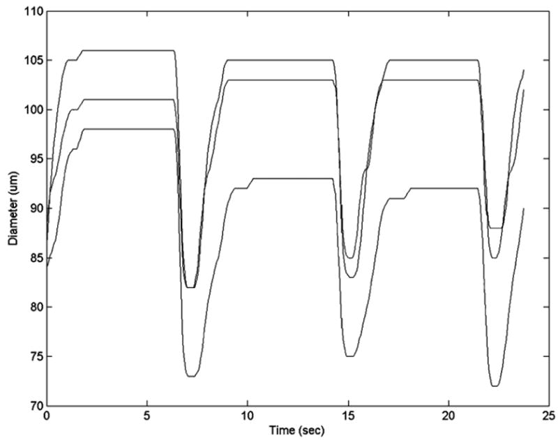
Diameter measurements taken at three different locations of the vessel (top, middle, and bottom). In this case the vessel narrows as you go from top to bottom, and the vessel also contracts more strongly at the bottom.

CONCLUSIONS

Through various experiments we have demonstrated the capability of image correlation approaches to measure fluctuations in diameter of contracting mesenteric lymphatics. While there are many well established approaches for measuring the diameter of vessels,^1,7,9 it was advantageous to measure them through our image correlation program. This ensured that our measurements could be used to optimize our ability to track lymph flow within the image correlation program by temporally adjusting the correlation window according to the vessel contractions. The program has proven to be quite robust at detecting temporal fluctuations in lymph flow. For all the cases that were tested, the actual velocity appears to be somewhere between the spatially averaged velocity and the maximum velocity, although its exact value depends on the radial distribution of the lymphocytes. This methodology will work quite well for future physiological studies, provided that the main parameter of interest is measuring temporal fluctuations in flow before and after various conditions are imposed on the vessel. While precise estimations of wall shear stress would be difficult for this approach due to the potential departures from purely Poiseuille flow (moving walls, large particles suspended in the fluid, etc.), temporal fluctuations in wall shear could be estimated, providing information that will be quite useful in future investigations of the flow induced inhibition of the lymphatic pump.

The lymphatics play important roles in lipid transport, removal of fluid from the tissue spaces, and immune cell trafficking. Currently, little work has been done in investigating the role of biomechanics (including flow among others) on this wide variety of lymphatic functions. Much of the lack of progress has been due to the limited number of tools available to study the lymphatic system. We are hopeful that the tools we have developed in these initial studies will accelerate the progress in lymphatic research and encourage others to join in the work.

References

- 1.Clough AV, Krenz GS, Owens M, Altinawi A, Dawson CA, Linehan JH. An algorithm for angio-graphic estimation of blood-vessel diameter. J Appl Physiol. 1991;71:2050–2058. doi: 10.1152/jappl.1991.71.5.2050. [DOI] [PubMed] [Google Scholar]
- 2.Dixon JB, Moore J, Jr, Coté GL, Gashev AA, Zawieja DC. Fluid velocity and wall shear stress in contracting mesenteric rat lymphatics in situ. Microcirculation. 2006 doi: 10.1080/10739680600893909. (in press) [DOI] [PubMed] [Google Scholar]
- 3.Dixon JB, Zawieja DC, Gashev AA, Coté GL. Measuring microlymphatic flow using fast video microscopy. J Biomed Optics. 2005;10:064016–1–064016–7. doi: 10.1117/1.2135791. [DOI] [PubMed] [Google Scholar]
- 4.Gashev AA, Davis MJ, Delp MD, Zawieja DC. Regional variations of contractile activity in isolated rat lymphatics. Microcirculation. 2004;11:477–492. doi: 10.1080/10739680490476033. [DOI] [PubMed] [Google Scholar]
- 5.Gashev AA, Davis MJ, Zawieja DC. Inhibition of the active lymph pump by flow in rat mesenteric lymphatics and thoracic duct. J Physiol. 2002;540:1023–1037. doi: 10.1113/jphysiol.2001.016642. [DOI] [PMC free article] [PubMed] [Google Scholar]
- 6.Please supply the reference details.
- 7.Molloi SY, Ersahin A, Roeck WW, Nalcioglu O. Absolute cross-sectional area measurements in quantitative coronary arteriography by dual-energy dsa. Invest Radiol. 1991;26:119–127. doi: 10.1097/00004424-199102000-00005. [DOI] [PubMed] [Google Scholar]
- 8.Tsukada K, Minamitani H, Sekizuka E, Oshio C. Image correlation method for measuring blood flow velocity in microcirculation: Correlation ’window’ simulation and in vivo image analysis. Physiol Measure. 2000;21:459–471. doi: 10.1088/0967-3334/21/4/303. [DOI] [PubMed] [Google Scholar]
- 9.Uyama C, Kita Y, Matsusita S. Optimal sampling interval and edge-detection algorithm for measurement of blood-vessel diameter on a cineangiogram. Invest Radiol. 1993;28:1128–1133. doi: 10.1097/00004424-199312000-00008. [DOI] [PubMed] [Google Scholar]